On the Emergence of Nonextensivity at the Edge of Quantum Chaos

Abstract

We explore the border between regular and chaotic quantum dynamics, characterized by a power law decrease in the overlap between a state evolved under chaotic dynamics and the same state evolved under a slightly perturbed dynamics. This region corresponds to the edge of chaos for the classical map from which the quantum chaotic dynamics is derived and can be characterized via nonextensive entropy concepts.

1 Introduction

Classical chaotic dynamics is identified by extreme sensitivity to initial conditions. Under chaotic dynamics, two arbitrarily close points in phase space diverge at an exponential rate, quantified by the Lyapunov exponent L+L . Non-chaotic dynamics does not show this extreme dependence on initial conditions, hence, the Lyapunov exponent is equal to zero. However, it has been conjectured, that, though the Lyapunov exponent may vanish, the system may have a positive generalized Lyapunov coefficient C3 describing power-law, rather than exponential, divergence of classical trajectories. This is the case, at the border between chaotic and non-chaotic dynamics (the ‘edge of chaos’) where the Lyapunov exponent goes to zero, but there remains a positive generalized Lyapunov coefficient.

This paper identifies a characteristic signature for the edge of quantum chaos. Quantum states maintain a constant overlap fidelity (heretofore referred to as the overlap or fidelity) , or distance, under all quantum dynamics, regular and chaotic. One way to characterize quantum chaos is to compare the evolution of an initially chosen state under the chaotic dynamics with the same state evolved under a perturbed dynamics P1 ; P2 ; SC . When the initial state is in a regular region of a mixed phase space system, a system whose phase space has regular and chaotic regions, the overlap remains close to one. When the initial state is in a chaotic region, the overlap decay is exponential. This paper explores the edge of quantum chaos, a region of polynomial overlap decay YSW1 .

This paper is structured as follows, we first give a short review of the Lyapunov description of chaotic dynamics and the lack of correspondence between this description and quantum dynamics. We then discuss suggested characteristics of quantum chaos (known as signatures of quantum chaos), concentrating on the overlap decay first introduced by Peres P1 ; P2 . Overlap decay proves to be a useful signature of quantum chaos from which to explore the border between regular and chaotic quantum dynamics. Next, we will review the nonextensive entropy form introduced in C1 and discuss its relevance to the edge of chaos phenomenon. Finally, we locate the ‘edge of quantum chaos’ in a mixed phase space system and, using the nonextensive entropy formalism, show how the overlap decay at the edge of quantum chaos depends on perturbation strength and Hilbert space dimension.

2 Classical Chaos

The Lyapunov exponent description of classical chaos is as follows L+L . Let $\Delta x$ be the distance between two points on phase space. We define $\xi=lim_{\Delta x(0)\rightarrow 0}(\frac{\Delta x(t)}{\Delta x(0)})$, to describe how far apart two initially arbitrarily close points on phase space become at some time $t$. Generally, $\xi(t)$ is the solution to the differential equation

$$\frac{d\xi(t)}{dt}=\lambda_{1}\xi(t),$$ (1)

giving the solution

$$\xi(t)=e^{\lambda_{1}t}$$ (2)

where $\lambda_{1}$ is the Lyapunov exponent (the use of the subscript will become clear later on). As seen from the above equation when the Lyapunov exponent is positive two arbitrarily close points on phase space diverge at an exponential rate. Thus, the dynamics described by $\xi(t)$ is strongly sensitive to initial conditions and we have chaotic dynamics.

3 Quantum Chaos

While the Lyapunov exponent description of chaos works well for points on a classical phase space it cannot hold true for quantum mechanical states or wavefunctions. A measure of distance between quantum wavefunctions is the overlap

$$O_{i}=\langle\Psi|\Phi\rangle.$$ (3)

However, the overlap between two quantum wavefunctions remains unchanged under unitary evolution governed by the linear Schrödinger equation. This is seen from

$$O(n)=\langle\Psi(U^{n})^{{\dagger}}U^{n}|\Phi\rangle=O_{i},$$ (4)

where $U$ is the unitary system evolution. Hence, the distance between two arbitrarily close quantum mechanical wavefunctions, like the distance between two Liouville probability densities, does not diverge and cannot be described by the Lyapunov exponent picture. This seeming lack of correspondence has led to the study of ‘quantum chaos,’ the search for characteristics of quantum dynamics that manifest themselves as chaotic in the classical realm B1 ; B2 ; H1 ; BGS .

Many such characteristics, quantum signatures of chaos, have been detailed in the literature and tested for quantum analogs of classically chaotic systems. These signatures can be divided into two broad categories, static signatures and dynamic signatures. Static signatures look at characteristics of the Hamiltonian or unitary operator governing the system. The conjecture is that the evolution operator of quantum chaotic systems have statistical properties similar to those of random matrices. Hence, quantum analogs of classically chaotic systems show level repulsion, that is, if the energy eigenvalues of the system are ordered, the difference between nearest neighbors would result in a histogram with a Wigner-Dyson distribution BGS and not of a Poisonnian distribution expected for regular systems. In addition, the magnitude of the elements of the eigenvectors of quantum chaotic operators follow $\chi^{2}_{\nu}$ distributionsZyc from appropriate random matrix ensemble.

Dynamic signatures of quantum chaos look at the evolution of a state under the quantum chaotic operator compared to the same evolution with some additional perturbation. An example of a dynamic signature of chaos is hypersensitivity to perturbation. For chaotic systems (both classical and quantum), the amount of information necessary to track the state of a system when the dynamics is interrupted by an unknown perturbation grows at an exponential rate with increasing time SC . Other signatures of quantum chaos look at the entropy growth of chaotic systems versus regular systems ZP1 .

4 Overlap Decay

Overlap decay as a signature of quantum chaos was first introduced by Peres P1 ; P2 ; P3 as a quantum analog of initial state sensitivity. Rather than look at two slightly different states and see how they evolve under a certain dynamics, Peres suggested looking at one state, $|\psi_{i}\rangle$, and see how it evolves under under two slightly different dynamics, an unperturbed Hamiltonian $H$, and the same Hamiltonian with a small perturbation $H+\delta V$, where $\delta$ is the perturbation strength. The overlap at time $t$ is

$$O(t)=|\langle\psi_{u}(t)|\psi_{p}(t)\rangle|.$$ (5)

where $|\psi_{u}(t)\rangle=e^{-iHt}|\psi_{i}\rangle$ and $|\psi_{p}(t)\rangle=e^{-i(H+\delta V)t}|\psi_{i}\rangle$ are the unperturbed and perturbed states, respectively. The initial behavior of the overlap shows different behavior depending on whether or not $H$ is chaotic. Recently, the study of overlap decay has seen a revival of interest which has served to identify several regimes of overlap decay behavior based on whether the system is chaotic or regular, the type and strength of perturbation, and the type of initial state. We note that many of the works cited use $O^{2}$ as the fidelity. Here, we follow Prosen and simply use the overlap, $O$.

For quantum chaotic systems, quantum versions of classically chaotic maps or random matrix models, there are several regions of behavior based on the strength of the perturbation. Perturbation strength is characterized by the size of a typical off diagonal element, $\sigma$, of the perturbation operator when the perturbation operator is written in the ordered eigenbasis of the unperturbed dynamics, $H$. If $\sigma$ is less than the average level spacing of the unperturbed system, $\Delta$, the perturbation is weak. If $\sigma>\Delta$, the perturbation is in the Fermi Golden Rule (FGR) regime Jacq ; Cerruti . The average level spacing is equal to $2\pi/N$ where $N$ is the dimension of the system Hilbert space. A typical off diagonal element of the perturbation operator in the ordered eigenbasis of the unperturbed system (where the unperturbed system is assumed to have eigenvector statistics of a random matrix see J ) is equal to $\sqrt{\delta^{2}\overline{V_{mn}^{2}}}$, where $\overline{V_{mn}^{2}}$ is the second moment of the matrix elements of the perturbation Hamiltonian.

For short enough time, the overlap decay is quadratic for any perturbation strength P1 . After this time, weak perturbations lead to a Gaussian overlap decay as expected from first order perturbation theory P3 . Perturbations in the FGR regime lead to an exponential decay of overlap whose rate, $\Gamma$, increases with perturbation strength. For many systems, $\Gamma$ increases as the perturbation strength squared Jacq , however, some systems do not show this exact dependence W1 . For systems with a classical analog, initial coherent states, and classical perturbations, $\Gamma$ will increase with perturbation strength until the decay rate reaches a value given by the Lyapunov exponent of the analog classical system Jacq ; Jala ; Cas . This is a wonderful example of a dynamical property of the classical system emerging in quantum mechanics. The increase $\Gamma$ may also saturate at the bandwidth of $H$ Jacq .

For initial states that are coherent or random states, the Gaussian or exponential behavior continues until the fidelity reaches a saturation point at $\simeq 1/N$. For initial states that are system eigenstates, there is no decay in the weak perturbation regime, and in the FGR regime there is an exponential decay of overlap which saturates at $\simeq 1/\Gamma$ W1 ; YSW2 .

Regular, non-chaotic, systems have a Gaussian decay in the FGR regime Prosen . The Gaussian decay is faster then the exponential decay of chaotic states. This result has been explained using correlation functions and may be understood as follows: a perturbation to a chaotic system is quickly spread out to the entire Hilbert space of the system. Repetition of the same perturbation does not lead to a compounded error (the correlation time is short). Regular systems, however, do not have this mechanism to spread out the perturbation. The same perturbation compounds the error (there is a long correlation time) leading to a faster fidelity decay. For some more complex regular systems, a power-law decay has also been observed Been .

Here we study a mixed system, a system with both chaotic and regular regimes. Coherent states within the regular regime are practically eigenstates of the system and the overlap of these states oscillates close to unity P2 ; Prosen , as shown in figure 1. Coherent states in the chaotic regime behave like other chaotic systems, they show exponential overlap decay in the FGR regime and Gaussian overlap decay for weak perturbations. We explore the border between the regular and chaotic regions and show that, in both the FGR and weak perturbation regimes, coherent states near this border have a polynomial overlap decay YSW1 .

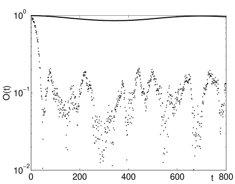
Figure 1: Overlap decay of coherent states in the regular and chaotic zone of the $J=480$ QKT with $k=3$ and $\delta=.005$ (in the FGR regime). The overlap of the coherent state centered at the fixed point of the classical kicked top is practically an eigenstate of the QKT and oscillates close to unity. The overlap of the coherent state in the chaotic zone decays first quadratically and then exponentially.

5 Nonextensive Entropy

The Boltzmann-Gibbs formulation of statistical mechanics is one of the pillars of modern day physics. However, its applicability, indeed its formulation, is only for systems with short range interactions. Self-gravitating systems and other systems such as those with long range forces, long range memories (non-Markovian), or multifractal structures present significant difficulties for the application of the Boltzmann-Gibbs formulation. In 1988, in an attempt to understand the nature of some of these systems, one of us C1 proposed the generalization of Boltzmann-Gibbs statistical mechanics on the basis of a generalized non-extensive entropy, $S_{q}$. When $q=1$, $S_{q}$ recovers the usual Boltzmann-Gibbs entropy.

The generalized entropy is given as follows:

$$S_{q}=k\frac{1-\sum^{W}_{i=1}p^{q}_{i}}{q-1}$$ (6)

where $k$ is a positive constant, $p_{i}$ is the probability of finding the system in microscopic state $i$, and $W$ is the number of possible microscopic states of the system; $q$ is the entropic index which characterizes the degree of the system nonextensivity. In the limit $q\to 1$ we recover the usual Boltzmann entropy

$$S_{1}=-k\sum^{W}_{i=1}p_{i}\;lnp_{i}.$$ (7)

To demonstrate how $q$ characterizes the degree of nonextensivity of a system, we present the $S_{q}$ entropy addition rule C2 . If $A$ and $B$ are two independent systems such that the probability $p(A+B)=p(A)p(B)$, the entropy of the total system $S_{q}(A+B)$ is given by the following:

$$\frac{S_{q}(A+B)}{k}=\frac{S_{q}(A)}{k}+\frac{S_{q}(B)}{k}+(1-q)\frac{S_{q}(A)S_{q}(B)}{k^{2}}.$$ (8)

From the above equation one can see that $q<1$ corresponds to superextensivity, the combined system entropy is more then the sum of the two independent systems; $q>1$ corresponds to subextensivity, the combined system entropy is less then the two independent systems. Using this entropy to generalize statistical mechanics and thermodynamics has helped to explain many natural phenomena in a wide range of fields.

One application of nonextensive entropy occurs in one dimensional dynamical maps. As explained above, when the Lyapunov exponent of a system is positive, the system dynamics is strongly sensitive to initial conditions and is called chaotic. When the Lyapunov exponent goes to zero it has been conjectured C3 (and proven for the logistic map robledo ) that the distance between two initially arbitrarily close points can be described by $\frac{d\xi}{dt}=\lambda_{q_{sen}}\xi^{q_{sen}}$ leading to $\xi=[1+(1-q_{sen})\lambda_{q_{sen}}t]^{1/(1-q_{sen})}$ (sen stands for sensitivity). This requires the introduction of $\lambda_{q_{sen}}$ as a generalized Lyapunov coefficient. The Lyapunov coefficient scales inversely with time as a power law instead of the characteristic exponential of a Lyapunov exponent. Thus, there exists a regime, $q_{sen}<1,\lambda_{1}=0,\lambda_{q_{sen}}>0$, which is weakly sensitive to initial conditions and is characterized by having power law, instead of exponential, mixing. This regime is called the edge of chaos.

The polynomial overlap decay found for initial states of a mixed system near the chaotic border are at the ‘edge of quantum chaos’, the border between regular and chaotic quantum dynamics. This region is the quantum analog of the classical region characterized by the generalized Lyapunov coefficient.

6 The Quantum Kicked Top

The system studied in this work is the quantum kicked top (QKT) H2 defined by the operator:

$$U_{QKT}=e^{-i\pi J_{y}/2\hbar}e^{-i\alpha J_{z}^{2}/2J\hbar}.$$ (9)

$J$ is the angular momentum of the top and $\alpha$ is the ‘kick’ strength. The representation is such that $J_{z}$ is diagonal. The classical version of the kicked top has either regular, mixed, or fully chaotic dynamics depending upon the kick strength. We work with a QKT of $\alpha=3$ whose classical analog has a mixed phase space, with clearly defined regions of chaotic and regular dynamics. The perturbed operator is simply a QKT with a stronger kick strength $\alpha^{\prime}$. Hence, the perturbation operator, $V=\delta\pi J_{z}^{2}/2J$ where $\delta\equiv\alpha^{\prime}-\alpha$.

When $J$ is even the QKT has three invariant, dynamically independent subspaces P2 ; H2 . We can write basis functions for the invariant subspaces in terms of the eigenvectors of $J_{z}$ which, following Peres P2 , we will denote as $|m\rangle$. The ee subspace is even under a $180^{\circ}$ rotation about $x$ and even under a $180^{\circ}$ rotation about $y$ and has a Hilbert space dimension of $N=J/2+1$. The basis functions of the ee subspace are $|0\rangle$ and $(|2m\rangle+|-2m\rangle)/\sqrt{2}$, where $m$ ranges from 1 to $J/2$. The oo subspace is even under a $180^{\circ}$ rotation about $x$ and odd under a $180^{\circ}$ rotation about $y$ and $N=J/2$. Its basis functions are $(|2m-1\rangle-|1-2m\rangle)/\sqrt{2}$. The oe subspace is odd under a $180^{\circ}$ rotation about $x$, $N=J$, and has basis functions $(|2m\rangle-|-2m\rangle)/\sqrt{2}$ and $(|2m-1\rangle+|1-2m\rangle)/\sqrt{2}$. All of the numerical simulations in this work were done in the oo subspace of the QKT. This is to say, we construct the complete QKT and transform it into a basis such that it is block diagonal with the dimensions of the three blocks mentioned above. The columns of the transformation matrix $T$ to get the QKT operator into block diagonal form are the states which form the bases of the invariant subspaces. We take only the block corresponding to the oo subspace and use that as our map. The initial angular momentum coherent states are also transformed into this basis and, again, only the part of the state corresponding to the oo subspace is used.

The phase space of the classical kicked top is the unit sphere, $x^{2}+y^{2}+z^{2}=1$ and the resulting action of the map is:

$$\begin{array}[]{cc}x^{\prime}=&z\\ y^{\prime}=&x\;sin(\alpha z)+y\;cos(\alpha z)\\ z^{\prime}=&-x\;cos(\alpha z)+y\;sin(\alpha z).\end{array}$$ (13)

For $\alpha=3$ there are two fixed points of order one at the center of the regular regions. They are located at

$$x_{f}=z_{f}=\pm 0.6294126,\;y_{f}=0.4557187.$$ (14)

The regular and chaotic regions of the kicked top are clearly seen in the classical maps phase space shown in the figure 2.

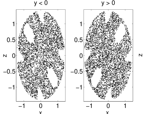
Figure 2: 10000 points of a chaotic orbit on the phase space of the classical kicked top with kick strength $\alpha=3$. The regular regions are clearly visible. The spherical phase space is projected onto the $x-z$ plane by multiplying the $x$ and $z$ coordinates of each point by $R/r$ where $R=\sqrt{2(1-|y|)}$ and $r=\sqrt{(1-y^{2})}$ P2 .

Hence, we expect quantum coherent states centered near the classical periodic point to exhibit significantly different behavior than coherent states centered in the classically chaotic region of the map. This is indeed seen in figure 1.

7 Locating the Edge of Quantum Chaos

To locate the edge of quantum chaos we use initial angular momentum coherent states keeping $y$ equal to $y_{f}$ of the positive fixed point for the classical kicked top and changing $z$ until a state which has a power-law overlap decay is found. The state which gives this behavior depends on the angular momentum of the QKT, $J$, but, given a fixed $J$, the power law emerges for perturbations in both the weak perturbation and FGR regimes. Examples of edge of quantum chaos behavior in both regimes is shown in figure 3 for a QKT of $J=240$. As seen in the figure, the power-law overlap decay is transitory between the quadratic and exponential behavior of the overlap decay. This transitory region does not appear for chaotic states (as shown in figure 1) or states close to the fixed point of the map, it is a signature of the ‘edge of quantum chaos.’

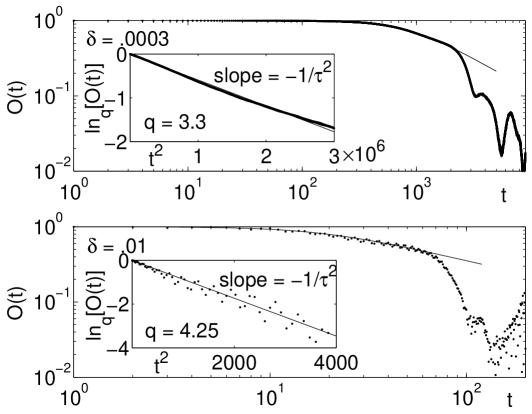
Figure 3: Overlap versus time for an initial angular momentum coherent state located at the border between regular and chaotic zones of the QKT of spin 240 and $\alpha=3$. This region, the edge of quantum chaos, shows the expected power law decrease in overlap. The top figure is for a perturbation strength in the weak perturbation regime, $\delta=.0003$ and the bottom figure is for a perturbation strength of $\delta=.01$, within the FGR regime. On the log-log plot the power law decay region, from about 600-2500 in the weak perturbation regime and 20-70 in the FGR regime, is linear. We can fit the decrease in overlap with the expression $[1+(q_{rel}-1)(t/\tau_{q_{rel}})^{2}]^{1/(1-q_{rel})}$ where, in the weak perturbation regime, the entropic index $q_{rel}=3.3$ and $\tau_{q_{rel}}=1300$ and in the FGR regime $q_{rel}=4.25$ and $\tau_{q_{rel}}=34$. The insets of both figures show $\ln_{q_{rel}}O\equiv(O^{1-q_{rel}}-1)/(1-q_{rel})$ versus $t^{2}$; since $\ln_{q}x$ is the inverse function of $e_{q}^{x}\equiv[1+(1-q)\;x]^{\frac{1}{1-q}}$, this produces a straight line with a slope $-1/\tau^{2}$ (also plotted).

The overlap decay for the edge of quantum chaos state is very well fit by the solution of the differential equation

$$dO/d(t^{2})=-O^{q_{rel}}/\tau_{q_{rel}}^{2}.$$ (15)

In the above equation, rel stands for relaxation which is an appropriate description of a $q>1$ phenomenon. In classical systems, $q_{rel}$ characterizes the relaxation of initial states towards an attractor. Although we do not know how to derive this differential equation from first principles, the numerical agreement is remarkable (see also borges ). A time-dependent $q$-exponential expression analogous to the one shown here has recently been proved for the edge of chaos and other critical points of the classical logistic map robledo .

Table 1: The edge of quantum chaos, the critical perturbation strength, $\delta_{c}$, and $q_{rel}^{c}$, the $q_{rel}$ for perturbations strengths below $\delta_{c}$, for explored values of $J$. As $J$ increases behavior characteristic of the edge of quantum chaos occurs further away from the fixed point of the classical map. The critical perturbation and $q_{rel}^{c}$ decrease with increased $J$.

J	Edge	$\delta_{c}$	$q_{rel}^{c}$
120	$z_{f}-.124$	$5.39\times 10^{-3}$	3.8
150	$z_{f}-.139$	$3.86\times 10^{-3}$	3.7
180	$z_{f}-.151$	$2.94\times 10^{-3}$	3.6
210	$z_{f}-.160$	$2.33\times 10^{-3}$	3.4
240	$z_{f}-.176$	$1.91\times 10^{-3}$	3.3
280	$z_{f}-.183$	$1.51\times 10^{-3}$	3.1
360	$z_{f}-.190$	$1.04\times 10^{-3}$	2.8
480	$z_{f}-.194$	$6.74\times 10^{-4}$	2.6

The values of $q_{rel}$ and $\tau_{q_{rel}}$ depend on the perturbation strength, $J$, and on whether the perturbation strength is in the weak perturbation or in the FGR regime. For perturbation strengths below the FGR regime, $\delta$ is less than some $\delta_{c}$, $q_{rel}$ remains constant at a value of $q_{rel}^{c}$. The transition into the FGR regime arises when the typical off diagonal elements of $V$ are larger than $\Delta$. We can approximate $\delta_{c}\simeq\sqrt{2\pi/N^{3}}$ Jacq where, in the $oo$ subspace of the kicked top $N=J/2$. Values for $\delta_{c}$ are shown in the above table. In the FGR regime $q_{rel}$ continues to increase with perturbation strength until a saturation perturbation, $\delta_{s}$, after which $q_{rel}=q_{rel}^{s}$ remains constant. As the top becomes more classical, with increased $J$, there is a decrease in $q_{rel}^{c}$ while in the weak perturbation regime, but an increase in the rate of increase of $q_{rel}$ while in the FGR regime. Because of this larger rate of increased $q_{rel}$ in the FGR regime, $q_{rel}^{s}$ increases with increasing $J$. However, we see that this is not the case for the $J=120$ case. For $J=120$, $q_{rel}$ increases beyond the expected saturation point. This may be due because the $J=120$ coherent state is so large that, at stronger perturbations, it leaks out of the regular region of the map in more than one place due to the odd shape of the regular region (see figure 6). The value of $\tau_{q_{rel}}$ decreases with perturbation strength and is well fit by a line of slope approximately -1 on a log-log plot; $\tau_{q_{rel}}$ also decreases with increasing $J$ at a fixed perturbation strength. The values of $q_{rel}$ and $\tau_{q_{rel}}$ for a number of different perturbation strengths can be seen in the figure 4.

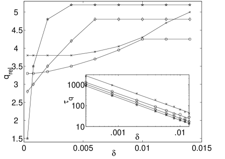
Figure 4: Values of $q_{rel}$ and $\tau_{q}$ (inset) for $J=120$ (x), 240 (circles), 360 (diamonds) and 480 (stars). $q_{rel}$ remains constant for perturbation strengths below the critical perturbation and above the saturation perturbation. In between $q_{rel}$ increases with a rate dependent on $J$. The values of $q_{rel}^{c}$, $q_{rel}^{s}$, $\delta_{c}$ and $\delta_{s}$ can be seen in the figure. In addition the rate of growth of $q_{rel}$ with increased perturbation strength can be seen. The inset shows a loglog plot of the value of $\tau_{q}$ versus $\delta$ for the above values of $J$. The data can be fit with a lines of slope -1.06, -1.03, -1.07, and -1.08 for $J=120$, 240, 360 and 480 (top to bottom).

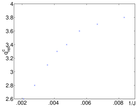
Figure 5: Values of $q_{rel}^{c}$ versus $1/J$. These are determined by exploring a number of perturbations much less than $\delta_{c}$.

The location of states exhibiting edge of quantum chaos behavior is not the same as the edge of chaos for the classical kicked top. This is due to the finite size of the coherent states. Though the coherent state may be centered at a point that is classically regular, some of the state may ’leak out’ into the chaotic region of the map. As $J$ increases the coherent state gets smaller and the quantum edge approaches the classical one. The location of the edge and the size of the coherent state compared to the regular regions of the map are shown in figure 6.

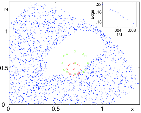
Figure 6: Coherent states of $J=120$ (circles) and $J=480$ (x) at the edge of quantum chaos superimposed on the upper right quarter of the classical phase space (shown in figure 2). The spherical phase space and ellipsoidal coherent states are projected onto the $x-z$ plane as described above. The $J=120$ coherent state is significantly larger then the $J=480$ coherent state, causing edge of quantum chaos behavior to appear for the $J=120$ wavefunction much closer to the classical periodic point than edge of chaos behavior for the $J=480$ wavefunction. The inset is a semilog ($y$-axis) plot of $1/J$ versus distance from the fixed point of the classical map. Note that the point of appearance of edge of chaos behavior follows an inverse power law with the size of the coherent state.

In conclusion, we have explored the region at the between chaotic and non-chaotic quantum dynamics, the edge of quantum chaos. Coherent states located at this border exhibit a power-law decrease in overlap as opposed to practically no decay for coherent states near the periodic point of the classical map and exponential overlap decay exhibited by fully chaotic quantum dynamics. This region is the quantum parallel of the classical region at the border between regular and chaotic classical dynamics where the Lyapunov exponent goes to zero and the mixing is characterized by the generalized Lyapunov coefficient. Further studies of this rich system are certainly welcome.

One of us (C.T.) acknowledges warm hospitality by H.-T. Elze and the organizers during the interesting meeting.

References

- (1) A.J. Lichtenberg and M.A. Lieberman Regular and Chaotic Dynamics (Springer Verlag, 1992).
- (2) C. Tsallis, A.R. Plastino, W.M. Zheng, Chaos, Solitons and Fractals 8, 885 (1997); M.L. Lyra, C. Tsallis, Phys. Rev. Lett. 80, 53 (1998); V. Latora, M. Baranger, A. Rapisarda, C. Tsallis, Phys. Lett. A, 273 97 (2000).
- (3) A. Peres, in Quantum Chaos, Quantum Measurement edited by H. A. Cerdeira, R. Ramaswamy, M. C. Gutzwiller, G. Casati (World Scientific, Singapore, 1991).
- (4) A. Peres, Quantum Theory: Concepts and Methods. Kluwer Academic Publishers (1995).
- (5) R. Schack, C.M. Caves, Phys. Rev. Lett. 71, 525 (1993). R. Schack, G.M. D’Ariano and C.M. Caves, Phys. Rev. E 50, 972 (1994); R. Schack, C.M. Caves, Phys. Rev. E 53, 3387 (1996); R. Schack, C.M. Caves, Phys. Rev. E 53, 3257 (1996).
- (6) Y.S. Weinstein, S. Lloyd, C. Tsallis, Phys. Rev. Lett. 89, 214101 (2002).
- (7) C. Tsallis, J. Stat. Phys. 52, 479 (1988). E.M.F. Curado, C. Tsallis, J. Phys. A 24, L69 (1991) [Corrigenda: 24, 3187 (1991) and 25, 1019 (1992)]. C. Tsallis, R.S. Mendes, A.R. Plastino, Physica A 261, 534 (1998).
- (8) M. V. Berry, Proc. R. Soc. London Ser. A 413, 183 (1987).
- (9) M. V. Berry in New Trends in Nuclear Collective Dynamics, edited by Y. A be, H. Horiuchi, and K Matsuyanagi (Springer, Berlin, 1992), p. 183.
- (10) F. Haake, Quantum Signatures of Chaos (Springer, New York, 1991).
- (11) O. Bohigas, M.J. Giannoni, C. Schmit, Phys. Rev. Lett. 52, 1, 1984.
- (12) F. Haake, K. Zyczkowski, Phys. Rev. A 42, 1013 (1990).
- (13) W.H. Zurek, J.P. Paz, Physica D, 83, 300-308, 1995.
- (14) A. Peres, Phys. Rev. A 30, 1610 (1984).
- (15) T. Prosen, M. Znidaric, J. Phys. A 35 1455, 2002.
- (16) Ph. Jacquod, P.G. Silvestrov, C.W.J. Beenakker, Phys. Rev. E 64, 055203 (2001)
- (17) N.R. Cerruti, S. Tomsovic, Phys. Rev. Lett. 88, (2002).
- (18) J. Emerson, Y.S. Weinstein, S. Lloyd, D.G. Cory, Phys. Rev. Lett. 89, 284102 (2002).
- (19) D. Wisniacki, nlin.CD/0208044.
- (20) R.A. Jalabert, H.M. Pastawski, Phys. Rev. Lett. 86, 2490 (2001); F.M. Cucchietti, C.H. Lewenkopf, E.R. Mucciolo, H.M. Pastawski, R.O. Vallejos Phys. Rev. E 65, 046209 (2002); F. Cucchietti, H.M. Pastawski, D. A. Wisniacki, Phys. Rev. E 65, 045206 (2002).
- (21) G. Benenti, G. Casati, Phys. Rev E 65, 066205 (2002).
- (22) Y.S. Weinstein, S. Lloyd, J. Emerson, D.G. Cory, Phys. Rev. Lett. 89, 157902 (2002).
- (23) Ph. Jacquod, I. Adagideli, C.W.J. Beenakker, Phys. Rev. Lett. 89, 154103 (2002).
- (24) C. Tsallis, Brazilian Journal of Physics 29, 1 (1999). Further reviews can be found in S. Abe and Y. Okamoto, eds., Nonextensive Statistical Mechanics and Its Applications, Series Lecture Notes in Physics (Springer-Verlag, Berlin, 2001); G. Kaniadakis, M. Lissia, A. Rapisarda, eds., Non Extensive Thermodynamics and Physical Applications, Physica A 305 (Elsevier, Amsterdam, 2002); M. Gell Mann, C. Tsallis, eds., Nonextensive Entropy–Interdisciplinary Applications, (Oxford University Press, Oxford, 2002), in press. A complete bibliography on the subject can be found at http://tsallis.cat.cbpf.br/biblio.htm.
- (25) F. Baldovin and A. Robledo, Europhys. Lett. 60, 518 (2002); F. Baldovin and A. Robledo, Phys. Rev. E 66, R045104 (2002); F. Baldovin and A. Robledo, cond-mat/0304410.
- (26) F. Haake, M. Kus, R. Scharf, Z. Phys. B, 65, 381, 1987.
- (27) E.P. Borges, C. Tsallis, G.F.J. Ananos, P.M.C. Oliveira, Phys. Rev. Lett. 89, 254103 (2002).