Measurement-induced Nonlinearity in Linear Optics

Abstract

We investigate the generation of nonlinear operators with single photon sources, linear optical elements and appropriate measurements of auxiliary modes. We provide a framework for the construction of useful single-mode and two-mode quantum gates necessary for all-optical quantum information processing. We focus our attention generally on using minimal physical resources while providing a transparent and algorithmic way of constructing these operators.

I Introduction

In recent years we have the seen signs of a new technological revolution in information processing, a revolution caused by a paradigm shift to information processing using the laws of quantum physics dowling02 . Since the pioneering work of Feynman feymann82 , Deutsch deutsch85 , and Shor shor95 a significant effort has occurred worldwide to develop the tools necessary to realise such a revolution. There are many possible routes and architectures machines ; NielsenChuang available to develop these quantum information processing devices. It has long been thought that photons would be an extremely strong contender for realising some quantum information processing circuits milburn88 . Many of the photon’s properties, for instance easy manipulation, have made them ideal for this. However, for scalable quantum information processing we require photons to interact with one another. To achieve such interactions it was known that massive reversible nonlinearities would be required shen84 . Materials giving such large nonlinearities were thought to be (and are still) well beyond our ability to manufacture. Knill, Laflamme, and Milburn (KLM) however found a way to create such nonlinearities using only linear optical elements, single photon sources and detectors KLM . More precisely they showed how it is possible using such elements to perform conditionally the nonlinear transformation

$$|\Psi\rangle = c_{0}|0\rangle+c_{1}|1\rangle+c_{2}|2\rangle$$ (1)

$$\rightarrow c_{0}|0\rangle+c_{1}|1\rangle-c_{2}|2\rangle=|\Psi^{\prime}\rangle\,.$$

The optical circuit (depicted in Fig. 1) creating this nonlinear transformation uses ancilla modes, one prepared with a single photon present and the other empty. The nonlinearity was induced by definite measurements of the presence of the single photon and the vacuum state in the appropriate ancilla modes. This insight has reopened the door to all-optical quantum information processing. Other optical schemes footnote-1 have been proposed along the KLM line to generate such sign shifts ralph02a ; Ralph01 ; kok02 ; others . These operations are generally conditional in nature. By this we mean the transformation only works when the appropriate measurement results are obtained at the ancilla detectors. While this would seem to limit the viability of the information processing, it is straightforward however by using a teleportation-based protocol to turn such nondeterministic operations into deterministic ones gottesman99 ; KLM .

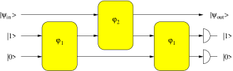
Figure 1: Schematic setup of the KLM circuit for generating a nonlinear sign shift using 3 beam-splitters, a single photon source and single photon resolving detectors.

There have been a number of key experiments demonstrating elements of linear optical information processing pittman02 ; pittman02a ; pittman03 . These have generally focused on the technology necessary to perform single-qubit rotations and CNOT gates. Such gates are well known to be sufficient to perform universal computation (they are the minimum set required). From these primitive elements interesting devices such as Quantum Repeaters kok02a and single-photon quantum non-demolition detectors kok02 can be created. In this paper we wish to shift the focus slightly. Instead of using only these primitive gates we will investigate what operations can be constructed from linear elements, single photon sources, and detectors. This shift is analogous to the shift in classical computing from a RISC (reduced instruction set) architecture to the CISC (complex instruction set) architecture. The RISC-based architecture in quantum computing terms could be thought of as a device built only from the minimum set of gates while the CISC-based machine would be built from a much larger set, a natural set of gates allowed by the fundamental resources.

Our primary focus in this paper will be on the operations that can be constructed from the linear optics set. We show how to construct general operators that can be applied to the required input states. We further indicate what operations are easily constructed and what are potentially difficult, illustrating our constructive procedure with examples from one-mode and two-mode situations. Our constructive procedure can easily be applied to multiple modes. The inputs to the computational modes do not need to be restricted to qubits only: the operations can be applied onto qudits and continuous variables just as easily.

This paper is organised as follows. In Sec. II we will derive some general expressions necessary for the construction of useful nonlinear operations. In Sec. III we will be concerned with single-mode operations, followed by two-mode operations in Sec. IV. Until then, we assume perfect beam splitters and detections which is an oversimplification, indeed. We will therefore focus on the effects of absorption and non-unit detection efficiencies in Sec. VI before drawing some conclusions in Sec. VII. Some useful formulae regarding permanents of unitary matrices can be found in the Appendix.

II General beam-splitter transformation

In order to introduce the notation we will be using throughout the paper we will briefly review the most basic features of quantum-state transformation by a lossless beam splitter. We refer the reader to the extensive literature for details beamsplitter . Every (lossless) beam splitter can be thought of as a unitary operator on the level of photonic creation and annihilation operators of the incoming and outgoing fields, i.e.

$$\hat{\bm{b}}=\hat{U}^{\dagger}\hat{\bm{a}}\hat{U}=\bm{\Lambda}\hat{\bm{a}}\,,\quad\hat{\bm{a}}={\hat{a}_{1}\choose\hat{a}_{2}}\,,\quad\hat{\bm{b}}={\hat{b}_{1}\choose\hat{b}_{2}}\,,$$ (2)

where $\hat{U}$ is a unitary operator and $\bm{\Lambda}$ the associated unitary matrix [$\bm{\Lambda}\in$ SU(2)]. The transformation matrix $\bm{\Lambda}$ consists of the transmission and reflection coefficients $T$ and $R$ and can be given in the form

$$\bm{\Lambda}=\left(\begin{array}[]{cc}T&R\\ -R^{\ast}&T^{\ast}\end{array}\right)\,.$$ (3)

Unitarity of $\bm{\Lambda}$ requires $|T|^{2}+|R|^{2}=1$ which leads to the usual definition of the beam splitter ‘angle’ $\varphi$ by writing $|T|=\cos\varphi$, $|R|=\sin\varphi$. The unitary operator $\hat{U}$ can be given in several equivalent forms, two of which are the following:

$$\hat{U} = e^{-i\hat{\bm{a}}^{\dagger}\bm{\Phi}\hat{\bm{a}}}\,,\quad\bm{\Lambda}=e^{-i\bm{\Phi}}\,,$$ (4)

$$\hat{U} = T^{\hat{n}_{1}}e^{-R^{\ast}\hat{a}_{2}^{\dagger}\hat{a}_{1}}e^{R\hat{a}_{1}^{\dagger}\hat{a}_{2}}T^{-\hat{n}_{2}}\,.$$ (5)

The effect of the beam splitter cannot only be described by transforming the photonic operators, but equivalently by transforming the quantum state $\hat{\varrho}$ as

$$\hat{\varrho}_{\text{out}}=\hat{U}\hat{\varrho}_{\text{in}}\hat{U}^{\dagger}\,.$$ (6)

Noting that the input density operator $\hat{\varrho}_{\text{in}}$ can be written as a functional of photonic creation and annihilation operators, $\hat{\varrho}_{\text{in}}=\hat{\varrho}_{\text{in}}[\hat{\bm{a}},\hat{\bm{a}}^{\dagger}]$, the quantum-state transformation can be represented as

$$\hat{\varrho}_{\text{out}}=\hat{\varrho}_{\text{in}}\left[\hat{U}\hat{\bm{a}}\hat{U}^{\dagger},\hat{U}\hat{\bm{a}}^{\dagger}\hat{U}^{\dagger}\right]=\hat{\varrho}_{\text{in}}\left[\bm{\Lambda}^{+}\hat{\bm{a}},\bm{\Lambda}^{T}\hat{\bm{a}}^{\dagger}\right]\,,$$ (7)

that is, the state transforms with the inverse operator plk1 ; stenholm1 . On the level of quantum states we thus have to perform the replacements

$$\hat{\bm{a}} \mapsto \bm{\Lambda}^{+}\hat{\bm{a}}\,,$$ (8)

$$\hat{\bm{a}}^{\dagger} \mapsto \bm{\Lambda}^{T}\hat{\bm{a}}^{\dagger}\,.$$ (9)

We will use Eq. (9) extensively throughout the paper.

Suppose we were given an input state with $N$ modes with the associated creation and annihilation operators labelled by $\hat{a}_{i}^{(\dagger)}$, $i=1\dots N$. Additionally, we have a supply of $M$ auxiliary modes labelled by $\hat{a}_{j}^{(\dagger)}$, $j=N+1,\ldots,N+M$. Then, a general unitary transformation on all the modes maps $\hat{\bm{a}}^{\dagger}\mapsto\bm{\Lambda}^{T}\hat{\bm{a}}^{\dagger}$, $\bm{\Lambda}\in\text{SU}(N+M)$. What we mean precisely by SU($N+M$) is a unitary operator on the level of photonic creation and annihilation operators in $N+M$ dimensions. In what follows, we will only make use of the unitarity of the corresponding matrices and will not further elaborate on the actual underlying group structure. In order to construct our quantum operations we will use the decomposition of an arbitrary element of the group SU($N$) into at most $N(N-1)/2$ U(2) group elements, i.e. beam splitters Reck94 .

First, let us define our notation. By $|0\rangle^{\otimes N}$ we mean the tensor product state $|0\rangle_{1}|0\rangle_{2}\ldots|0\rangle_{N}$. Let the input state now be given in a functional form as

$$|\psi_{\text{in}}\rangle=\hat{f}(\hat{a}_{1}^{\dagger},\dots,\hat{a}_{N}^{\dagger})|0\rangle^{\otimes N}$$ (10)

and the auxiliary state in product form as

$$|\psi_{\text{aux}}\rangle=\prod\limits_{j=N+1}^{N+M}\frac{\left(\hat{a}_{j}^{\dagger}\right)^{m_{j}}}{\sqrt{m_{j}!}}|0\rangle^{\otimes M}\,.$$ (11)

Here $m_{j}$ is a non-negative integer that represents the number of photons initially in the mode $j$. Finally, the state we project on shall be denoted by

$$|\psi_{\text{proj}}\rangle=\prod\limits_{j=N+1}^{N+M}\frac{\left(\hat{a}_{j}^{\dagger}\right)^{n_{j}}}{\sqrt{n_{j}!}}|0\rangle^{\otimes M}\,.$$ (12)

where $n_{j}$ represents the number of photons in the projected mode $j$. The output state after mixing at the beam splitter network and projecting onto $|\psi_{\text{proj}}\rangle$ looks then as

$$|\psi_{\text{out}}\rangle \propto \langle\psi_{\text{proj}}|\hat{U}|\psi_{\text{aux}}\rangle\otimes|\psi_{\text{in}}\rangle$$ (13)

$$= {}^{M\otimes}\langle 0|\prod\limits_{i,j=N+1}^{N+M}\frac{\left(\hat{a}_{i}\right)^{n_{i}}}{\sqrt{n_{i}!m_{j}!}}\left(\sum\limits_{k=1}^{N+M}\Lambda_{kj}\hat{a}_{k}^{\dagger}\right)^{m_{j}}\hat{f}\left(\sum\limits_{l=1}^{N+M}\Lambda_{l1}\hat{a}_{l}^{\dagger},\dots,\sum\limits_{l=1}^{N+M}\Lambda_{lN}\hat{a}_{l}^{\dagger}\right)|0\rangle^{\otimes N+M}\,.$$

What we see here is that the effect of the beam splitter network is to generate the desired mixing of the photonic creation operators of signal and auxiliary modes. Now we make use of the ordering formula well-known from bosonic operator algebras (see, e.g., VogelWelsch ; Louisell )

$$\left[\hat{a},F(\hat{a},\hat{a}^{\dagger})\right]=\frac{\partial}{\partial\hat{a}^{\dagger}}F(\hat{a},\hat{a}^{\dagger})$$ (14)

to rewrite the output state as

$$|\psi_{\text{out}}\rangle\propto{}^{M\otimes}\langle 0|\prod\limits_{i,j=N+1}^{N+M}\frac{\left(\hat{a}_{i}\right)^{n_{i}}}{\sqrt{n_{i}!m_{j}!}}\left(\sum\limits_{k=1}^{N+M}\Lambda_{kj}\hat{a}_{k}^{\dagger}\right)^{m_{j}}\hat{f}\left(\sum\limits_{l=1}^{N+M}\Lambda_{l1}\hat{a}_{l}^{\dagger},\dots,\sum\limits_{l=1}^{N+M}\Lambda_{lN}\hat{a}_{l}^{\dagger}\right)|0\rangle^{\otimes N+M}\,.$$ (15)

Furthermore, we expand the function $\hat{f}(\hat{a}_{1}^{\dagger},\dots,\hat{a}_{N}^{\dagger})$ in a Taylor series as

$$\hat{f}(\hat{a}_{1}^{\dagger},\dots,\hat{a}_{N}^{\dagger})=\sum\limits_{p_{1},\ldots,p_{N}=1}^{N}c_{p_{1},\ldots,p_{N}}\frac{\left(\hat{a}_{1}^{\dagger}\right)^{p_{1}}}{\sqrt{p_{1}!}}\cdots\frac{\left(\hat{a}_{N}^{\dagger}\right)^{p_{N}}}{\sqrt{p_{N}!}}\,.$$ (16)

where $c_{p_{1},\ldots,p_{N}}$ is constrained in such a way that $\sum\limits_{p_{1},\ldots,p_{N}=1}^{N}|c_{p_{1},\ldots,p_{N}}|^{2}=1$. In that way we obtain the action of a SU($N+M$)-network in a quite general way. In general, this can be a laborious task. In order to see the structure behind it, let us focus first onto single-mode signal states. That is, the input state will be

$$|\psi_{\text{in}}\rangle = \hat{f}(\hat{a}_{1}^{\dagger})|0\rangle$$ (17)

$$= \sum\limits_{m}\frac{c_{m}}{\sqrt{m!}}\left(\hat{a}_{1}^{\dagger}\right)^{m}|0\rangle$$ (18)

and the network will represent an element of the group SU($N+1$).

In what follows we will restrict ourselves to the important special case when our resources consist of single photons and single-photon detectors. In this case, we can derive a number of interesting results. Let us first start with a very simple (and in fact well-known) example, a single beam splitter. Feeding a single photon in one input arm of the beam splitter and measuring a single photon leaving one output port of the beam splitter, we have in fact created the conditional non-unitary operator [using Eq. (5)] CondMeas

$$\hat{Y}=\langle 1_{2}|\hat{U}|1_{2}\rangle=T^{\hat{n}_{1}-1}\left[|T|^{2}-\hat{n}_{1}|R|^{2}\right]$$ (19)

acting on some signal state $|\psi_{\text{in}}\rangle$ (see Fig. 2). This is a very special result and probably the simplest non-unitary operator one can actually generate. This conditional operator has already been realised in an experiment Lvovsky where it is called ‘quantum-optical catalysis’.

Figure 2: Schematic setup for generating the simplest non-unitary conditional operator with a single-photon input and a single-photon detection.

In the following we will present some results on the general structure of conditional non-unitary operators.

Proposition 1: Let us suppose all $N$ auxiliary modes are prepared in single-photon states, and all $N$ detectors measure vacuum. This is equivalent to acting with an operator $\sim\left(\hat{a}_{1}^{\dagger}\right)^{N}$ on the signal state (left figure in Fig. 3).
Proof: The auxiliary and detected states are

$$|\psi_{\text{aux}}\rangle=\prod\limits_{i=2}^{N+1}\hat{a}_{i}^{\dagger}|0\rangle^{\otimes N}\,,\quad|\psi_{\text{det}}\rangle=|0\rangle^{\otimes N}\,.$$ (20)

The conditional (un-normalised) output state is therefore

$$|\psi_{\text{out}}\rangle \propto \sum\limits_{m}\frac{c_{m}}{\sqrt{m!}}$$ (21)

$${}^{N\otimes}\langle 0|\left(\prod\limits_{i=2}^{N+1}\sum\limits_{j=1}^{N+1}\Lambda_{ji}\hat{a}_{j}^{\dagger}\right)\left(\sum\limits_{k=1}^{N+1}\Lambda_{k1}\hat{a}_{k}^{\dagger}\right)^{m}|0\rangle^{\otimes N+1}$$

$$= \sum\limits_{m}\frac{c_{m}}{\sqrt{m!}}\left(\prod\limits_{i=2}^{N+1}\Lambda_{1i}\right)\Lambda_{11}^{m}\left(\hat{a}_{1}^{\dagger}\right)^{m+N}|0\rangle$$

$$= \left(\prod\limits_{i=2}^{N+1}\Lambda_{1i}\right)\left(\hat{a}_{1}^{\dagger}\right)^{N}\sum\limits_{m}\frac{c_{m}}{\sqrt{m!}}\Lambda_{11}^{m}\left(\hat{a}_{1}^{\dagger}\right)^{m}|0\rangle$$

$$= \left(\prod\limits_{i=2}^{N+1}\Lambda_{1i}\right)\left(\hat{a}_{1}^{\dagger}\right)^{N}\Lambda_{11}^{\hat{n}_{1}}|\psi_{\text{in}}\rangle\,.$$

Apart from normalisation (or success probability), which depends on the chosen input state, the output state is proportional to the $N$-fold application of the creation operator.

In complete analogy, we can prove the following:

Proposition 2: Let us suppose all $N$ auxiliary modes are prepared in the vacuum state and each of the $N$ detectors measures a single photon. Then, this is equivalent to acting with $\hat{a}_{1}^{N}$ on the input state (right figure in Fig. 3).

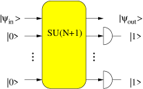
Figure 3: Adding (subtracting) photons to (from) the signal mode by subtracting (adding) the corresponding number of photons from (to) the auxiliary modes.

Proof: Again, let us first write down the auxiliary and the detected state:

$$|\psi_{\text{aux}}\rangle=|0\rangle^{\otimes N}\,,\quad|\psi_{\text{det}}\rangle=\prod\limits_{i=2}^{N+1}\hat{a}_{i}^{\dagger}|0\rangle^{\otimes N}\,.$$ (22)

Acting on the input state gives

$$|\psi_{\text{out}}\rangle \propto \sum\limits_{m}\frac{c_{m}}{\sqrt{m!}}$$ (23)

$${}^{N\otimes}\langle 0|\left(\prod\limits_{i=2}^{N+1}\hat{a}_{i}\right)\left(\sum\limits_{k=1}^{N+1}\Lambda_{k1}\hat{a}_{k}^{\dagger}\right)^{m}|0\rangle^{\otimes N+1}$$

$$=\sum\limits_{m}\frac{c_{m}}{\sqrt{m!}}{}^{\otimes N}\langle 0|\left(\prod\limits_{i=2}^{N+1}\frac{\partial}{\partial\hat{a}_{i}^{\dagger}}\right)\left(\sum\limits_{k=1}^{N+1}\Lambda_{k1}\hat{a}_{k}^{\dagger}\right)^{m}|0\rangle^{\otimes N+1}$$

$$=\sum\limits_{m}\frac{c_{m}}{\sqrt{m!}}\frac{m!}{(m-N)!}\left(\prod\limits_{i=2}^{N+1}\Lambda_{i1}\right)\Lambda_{11}^{m-N}\left(\hat{a}_{1}^{\dagger}\right)^{m-N}|0\rangle$$

$$=\left(\prod\limits_{i=2}^{N+1}\Lambda_{i1}\right)\Lambda_{11}^{\hat{n}_{1}}\hat{a}_{1}^{N}|\psi_{\text{in}}\rangle\,,$$

where in the last line we have repeatedly made use of the formula

$$\left(\hat{a}^{\dagger}\right)^{p}|0\rangle=\frac{1}{p+1}\hat{a}\left(\hat{a}^{\dagger}\right)^{p+1}|0\rangle$$ (24)

which immediately follows from the commutation relations of the photonic operators. This proves that, indeed, measuring $N$ photons from an $N$-mode auxiliary vacuum input is equivalent to acting $N$ times with the annihilation operator on the signal state.

Propositions 1 and 2 show how to generate arbitrary powers of creation and annihilation operators. In fact, one could have already guessed the general form of these operators by recalling that the network is represented by an element of the compact group SU($N+1$). Compactness of the group translates into photon-number conservation which is why adding (subtracting) $N$ photons from the auxiliary modes must end up as subtracting (adding) photons from (to) the signal mode. Note that in both cases only the matrix elements $\Lambda_{i1}$ or $\Lambda_{1i}$ ($i=2,\ldots,N+1$), respectively, appear. This means that the network decouples into a sequence of $N$ disconnected beam splitters. That is already the minimal number of beam splitters necessary for the generation of the wanted operators.

The next step consists of showing how powers of the number operator can be realised. In fact, an obvious way would be to combine the results from Propositions 1 and 2 and to construct an alternating network producing sufficient numbers of creation and annihilation operators. This might not be the most sensible way to do. In fact, as we will see later, the following result has much stronger implications for the construction of interesting quantum operations.

Proposition 3: Measuring single photons in all $N$ detectors from a supply of $N$ single-photon auxiliary state amounts to multiplying the input state with a polynomial of $N$th degree in the number operator, $P_{N}(\hat{n}_{1})$ (Fig. 4).
Proof: We will only sketch this proof and calculate the highest power of $\hat{n}_{1}$ and leave the remaining terms for an interested reader to calculate. Given that we choose the auxiliary and detected states of the form

$$|\psi_{\text{aux}}\rangle = \prod\limits_{i=2}^{N+1}\hat{a}_{i}^{\dagger}|0\rangle^{\otimes N}\,,$$

$$|\psi_{\text{det}}\rangle = \prod\limits_{k=2}^{N+1}\hat{a}_{j}^{\dagger}|0\rangle^{\otimes N}\,,$$ (25)

the output state can be written in the following way:

$$|\psi_{\text{out}}\rangle \propto \sum\limits_{m}\frac{c_{m}}{\sqrt{m!}}{}^{N\otimes}\langle 0|\left(\prod\limits_{k=2}^{N+1}\frac{\partial}{\partial\hat{a}_{k}^{\dagger}}\right)\left[\prod\limits_{j=2}^{N+1}\left(\sum\limits_{i=1}^{N+1}\Lambda_{ij}\hat{a}_{i}^{\dagger}\right)\right]\left(\sum\limits_{n=1}^{N+1}\Lambda_{n1}\hat{a}_{n}^{\dagger}\right)^{m}|0^{\otimes N+1}$$ (26)

$$= \left(\prod\limits_{j=2}^{N+1}\Lambda_{1j}\right)\left(\prod\limits_{n=2}^{N+1}\Lambda_{n1}\right)\frac{\hat{n}_{1}!}{(\hat{n}_{1}-N)!}\Lambda_{11}^{\hat{n}_{1}-N}|\psi_{\text{in}}\rangle+\ldots+\left(\sum\limits_{j=2}^{N+1}\prod\limits_{i\in{\cal P}}\Lambda_{ji_{\cal P}}\right)\Lambda_{11}^{\hat{n}_{1}}|\psi_{\text{in}}\rangle\,.$$

In the first term the factorial $\hat{n}_{1}!/(\hat{n}_{1}-N)!$ is a polynomial of order $N$ in $\hat{n}_{1}$ and thus the desired result. All other terms (not written except for the last, in lowest order in $\hat{n}_{1}$) contain lower-degree polynomials footnote-2 . This proves the assertion.

Figure 4: Generating polynomials of photon-number operators by single-photon inputs and detections.

The simplest example of this proposition is a single beam splitter the result of which we have already seen in Eq. (5). However, with the above propositions, we can immediately generalise our considerations to obtain the following results:

1. Given that the following for ancilla and detected modes

   $$\begin{array}[]{rcl}|\psi_{\text{aux}}\rangle&=&|1\rangle^{\otimes N+M}\\ |\psi_{\text{det}}\rangle&=&|1\rangle^{\otimes N}\otimes|0\rangle^{\otimes M}\end{array}\,,$$

   the output state will be

   $$|\psi_{\text{out}}\rangle\propto(\hat{a}_{1}^{\dagger})^{M}P_{N}(\hat{n}_{1})|\psi_{\text{in}}\rangle\,.$$

   We immediately see that this procedure has allowed us to act on the input state with the creation operator $(\hat{a}_{1}^{\dagger})^{M}$.

2. Analogously, with

   $$\begin{array}[]{rcl}|\psi_{\text{aux}}\rangle&=&|1\rangle^{\otimes N}\otimes|0\rangle^{\otimes M}\\ |\psi_{\text{det}}\rangle&=&|1\rangle^{\otimes N+M}\end{array}\,,$$

   the output state will be

   $$|\psi_{\text{out}}\rangle\propto P_{N}(\hat{n}_{1})(\hat{a}_{1})^{M}|\psi_{\text{in}}\rangle\,.$$

In both situations we have, with the aid of linear optics, single photon sources and detectors, been able to operate on the input state $|\psi_{\text{in}}\rangle$ with both $\hat{a}_{1}^{M}$ and $(\hat{a}_{1}^{\dagger})^{M}$. Let us now turn our attention to single-mode operations that are of interest in connection with quantum information processing.

III Single-mode operations

From now on we will focus onto the generation of unitary operators which are of utmost importance for most quantum information processing tasks. For all unitary operators it is easy to define the success probability, since unitary operators leave the norm of a quantum state unchanged. Since these operators $\hat{Y}$ are prepared conditionally, the success probability is just

$$p_{\text{success}}=\|\hat{Y}|\psi\rangle\|^{2}$$ (27)

for any (normalised) state vector $|\psi\rangle$.

We can derive some interesting results about these unitary operators. For example, let us suppose our input state is a single-mode state consisting only of elements in the zeroth and first Fock layer. It is clear that all operations on $|\psi_{\text{in}}\rangle$ of the type

$$|\psi_{\text{in}}\rangle=c_{0}|0\rangle+c_{1}|1\rangle\to c_{0}|0\rangle+e^{i\varphi}c_{1}|1\rangle$$ (28)

can be realised with a probability of $p=1$, since unitary operations simply consist of phase shifts of the $|1\rangle$ state. A special example with $\varphi\!=\!\pi$ is the Pauli-$\hat{\sigma}_{z}$. Going one step further we may ask what the conditions are for generation of unitary operations on single-mode states with up to two photons. It is reasonable to assume that we would need at least an SU(3)-network, that is, two auxiliary modes. In fact, we find that every unitary single-mode operator acting on states with up to two photons, separately in each Fock layer, can be generated by an SU(3)-network with two single-photon inputs and two single-photon detections. In order to show that, let us first calculate the conditional operator for the SU(3)-network with $|\psi_{\text{aux}}\rangle=|\psi_{\text{det}}\rangle=|11\rangle$. We get

$$\hat{Y}|\psi_{\text{in}}\rangle = \mbox{per }\bm{\Lambda}(1|1)|0\rangle+\mbox{per }\bm{\Lambda}|1\rangle$$

$$+\left(2\Lambda_{11}\mbox{per }\bm{\Lambda}-\Lambda_{11}^{2}\mbox{per }\bm{\Lambda}(1|1)+2\Lambda_{12}\Lambda_{21}\Lambda_{13}\Lambda_{31}\right)|2\rangle\,.$$

It is known that the range of $\mbox{per }\bm{\Lambda}$ (as a function of all its relevant parameter) is the unit disk in the complex plane Minc (see Appendix). In fact, so is the range of any principal sub-permanent $\mbox{per }\bm{\Lambda}(i|i)$. This can be seen from the decomposition of an SU(3)-matrix in terms of a product of three SU(2)-matrices Reck94 which themselves have a range spanning the unit disk. Therefore, it is immediately clear that we can again generate any phase $e^{i\varphi_{1}}$ between the states $|0\rangle$ and $|1\rangle$. As for the two-photon Fock layer, we can rewrite the coefficient in Eq. (III) to obtain a condition on the matrix $\bm{\Lambda}$ as

$$\mbox{per }\bm{\Lambda}(1|1)\left[e^{i\varphi_{2}}+\Lambda_{11}^{2}-2\Lambda_{11}e^{i\varphi_{1}}\right]=2\Lambda_{12}\Lambda_{21}\Lambda_{13}\Lambda_{31}\,,$$ (30)

where $e^{i\varphi_{2}}$ is the phase shift between $|0\rangle$ and $|2\rangle$. The modulus of the rhs of Eq. (30) can be shown to be bounded from above by $8/(27|\Lambda_{11}|^{2})$ by noting that $\prod_{i}\Lambda_{1i}$ is the product of the elements of a unit vector. Noting also that the principal sub-permanent $\mbox{per }\bm{\Lambda}(1|1)$ can take any value across the unit disk we can conclude that Eq. (30) has always a solution. This in turn means that every unitary single-mode operator acting within Fock layers on states with up to two photons can be generated by an SU(3)-network with two single-photon inputs and two single-photon detections which was to be proven. The probability of success is $|\mbox{per }\bm{\Lambda}(1|1)|^{2}$. It is also possible however to create certain phase shifts with the necessity for two ancilla photons. For instance, in KLM it was shown that a sign shift on the $|2\rangle$ Fock state only is possible with the ancilla state $|10\rangle$.

IV Two-mode operations

In order to do something useful in terms of quantum information processing, we have to operate on two modes simultaneously. This can be done in more than one way. For example, one can simply generalise the theory presented above for a single signal mode to more than one signal mode. It turns out that this is not a very transparent way. We will follow another route instead and decompose the two-mode operation into three subsequent steps:

1. combine the two modes at a beam splitter,

2. act on both modes separately,

3. and recombine the modes at another beam splitter.

The effect of the beam splitters is to mix the modes and to make them accessible for a single-mode operation in such a way that we can apply the result in Sec. III.

IV.1 The ‘controlled-phase’ gate

We will illustrate this statement with an example. Consider the two-mode operator $\hat{C}_{\varphi}$ acting on qubits. Its truth table is

$$|00\rangle \to |00\rangle\,,$$

$$|01\rangle \to |01\rangle\,,$$

$$|10\rangle \to |10\rangle\,,$$

$$|11\rangle \to e^{i\varphi}|11\rangle\,.$$ (31)

In terms of photon creation and annihilation operators the operator $\hat{C}_{\varphi}$ can be represented as

$$\hat{C}_{\varphi}=1-(1-e^{i\varphi})\hat{n}_{1}\hat{n}_{2}\,.$$ (32)

Now let us assume that we mix the signal modes at a symmetric beam splitter. The operator $\hat{C}_{\varphi}$ acts only in the two-photon Fock layer. Then it is very easy to see that with (nonlinear) single-mode operators $\hat{N}_{i}=1-\frac{1}{2}(1-e^{i\varphi})\hat{n}_{i}(\hat{n}_{i}-1)$, $i=1,2$, we achieve a transformation of an input state

$$|\psi_{\text{in}}\rangle=c_{00}|00\rangle+c_{01}|01\rangle+c_{10}|10\rangle+c_{11}|11\rangle$$ (33)

into

$$\hat{C}_{\varphi}|\psi_{\text{in}}\rangle=c_{00}|00\rangle+c_{01}|01\rangle+c_{10}|10\rangle+c_{11}e^{i\varphi}|11\rangle\,.$$ (34)

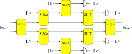
Figure 5: Controlled-phase gate with single-photon detectors only.

The nonlinear operator needed on both modes are polynomials of second degree in the number operators $\hat{n}_{i}$ and can thus be prepared conditionally with two auxiliary modes prepared in single-photon Fock states on each side followed by double single-photon detection. Hence, the overall requirements are four single-photon sources, eight beam splitters, and four single-photon detectors. The generic network is shown in Fig. 5. The detectors all measure single photons. We can write down the conditional operator as

$$\hat{Y}|\psi_{\text{in}}\rangle = \mbox{per }\bm{\Lambda}(1|1)c_{0}|0\rangle+\mbox{per }\bm{\Lambda}c_{1}|1\rangle$$

$$+\left[2\Lambda_{12}\Lambda_{21}\Lambda_{13}\Lambda_{31}+2\mbox{per }\bm{\Lambda}-\Lambda_{11}^{2}\mbox{per }\bm{\Lambda}(1|1)\right]c_{2}|2\rangle\,.$$

The success probability is $|\mbox{per }\bm{\Lambda}(1|1)|^{2}$. Numerically, we find values up to $p_{\text{success}}\approx 0.24$ in each interferometer arm.

However, it turns out that there is an even simpler network with only six beam splitters and two single-photon sources Ralph01 . It has the disadvantage, though, that one needs two vacuum detectors which are hard to make (and which are pretty inefficient). The corresponding network is shown in Fig. 6.

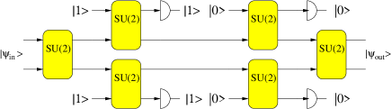
Figure 6: Controlled-$\hat{\sigma}_{z}$ gate with single-photon and vacuum detectors.

The set of beam splitters fed with vacuum states act as conditional phase shifts. In summary, we find that the beam splitters must satisfy

$$\arg T_{|1\rangle} = -\arg T_{|0\rangle}\,,$$ (36)

$$|T_{|1\rangle}| = 0.476\,,$$ (37)

$$|T_{|0\rangle}| = 0.87\,,$$ (38)

which gives a success probability of $p_{\text{success}}\approx 0.23$ in each arm, hence a total success probability of $\approx 0.05$.

Let us remark that the controlled-$\hat{\sigma}_{z}$ investigated by Ralph et al. Ralph01 falls into the same category as that described in our Fig. 5. The difference is that one of the single photons in each arm of the interferometer is replaced by the vacuum state and the single-photon detector by a vacuum detector vacuum-detector , respectively. This network corresponds to the following conditional operator:

$$\hat{Y}|\psi_{\text{in}}\rangle = \Lambda_{22}c_{0}|0\rangle+\mbox{per }\bm{\Lambda}(3|3)c_{1}|1\rangle$$ (39)

$$+(2\Lambda_{12}\Lambda_{21}\Lambda_{11}+\Lambda_{22}\Lambda_{11}^{2})c_{2}|2\rangle\,.$$

The probability of success is $|\Lambda_{22}|^{2}$. One needs to satisfy the set of conditions

$$\mbox{per }\bm{\Lambda}(3|3) = \Lambda_{22}\,,$$ (40)

$$2\Lambda_{12}\Lambda_{21}\Lambda_{11}+\Lambda_{22}\Lambda_{11}^{2} = -\Lambda_{22}\,,$$ (41)

from which it immediately follows that $\Lambda_{11}\!=\!1-\sqrt{2}$. The maximal value $|\Lambda_{22}|^{2}$ can take under the constraints (40) is then indeed 0.25 which is why the gate in Ref. Ralph01 is indeed optimal.

IV.2 The ‘swap’ gate

A somewhat more interesting operator is the swap operator $\hat{S}$ in the sense that here we encounter the first example of an operator that needs fewer resources than one would expect when considering CNOT and single-qubit rotations as building blocks for quantum circuits. It is known that it can be made from three CNOT operators $\hat{\not{C}}$ (equivalent to controlled-$\hat{\sigma}_{z}$ gates with attached Hadamard gates). Acting on qubits, one can write the photonic-operator version of it as

$$\hat{S}=\hat{n}_{1}\hat{n}_{2}+(\hat{n}_{1}-1)(\hat{n}_{2}-1)-\hat{a}_{1}^{\dagger}\hat{a}_{2}(\hat{n}_{1}-1)-\hat{a}_{2}^{\dagger}\hat{a}_{1}(\hat{n}_{2}-1)\,.$$ (42)

Let us see how the single-mode version of $\hat{S}$ can be derived. It is immediately clear that we have to act on the single-photon Fock layer only. It turns out that the nonlinear single-mode operators are

$$\hat{N}_{1} = 1+2\hat{n}_{1}(\hat{n}_{1}-2)\,,$$ (43)

$$\hat{N}_{2} = 1\,,$$ (44)

which means that we do nothing on mode 2, and we act with a polynomial of second degree in $\hat{n}_{1}$ on mode 1. Therefore, we would need only two single-photon sources, four beam splitters, and two single-photon detectors. However, the operator $\hat{N}_{1}$, when acting on Fock states $|n\rangle$, is nothing but a single-mode phase shift $(-1)^{\hat{n}_{1}}$. That is, the whole network collapses into a single $\pi$-phase plate in one arm of the Mach-Zehnder interferometer leaving us with just two beam splitters and one phase plate. This gate is remarkable in the sense that it is also unconditional, that is, it works deterministically with unit probability which makes it rather special.

These two simple examples show a general principle of constructing these networks. Both operators have in common that they act only within a specific Fock layer ($\hat{S}$: one photon; $\hat{C}_{\varphi}$: two photons). One then projects out all those Fock layers which are not affected by the operator. This leads to the polynomials in the number operators. The design of the polynomial coefficients in each case depend on the specific operation one wants to achieve.

IV.3 General considerations

A general conclusion can already be drawn from the results on one- and two-qubit operators: It is highly desirable to rewrite the quantum information network in such a way that the actual computation can be made as long as possible in the same Fock layers. Every crossing to another layer (cf. the Pauli operators $\hat{\sigma}_{x}$ and $\hat{\sigma}_{y}$) requires additional resources which might not be necessary. This leads us to state our main result of this paper:

Theorem: The generic operations that can be done easily and effectively with linear optics are operations within the same Fock layers. Let $M$ be the number of signal modes we want to operate on. Any $M$-qubit gate acting within Fock layers can be constructed with the help of generalised Mach–Zehnder interferometers with $M$ input and output ports ($2M$-ports for short) and at most $M$ conditional operators generating polynomials in the number operator of at most $M$th order (equivalent to SU($M+1$)-networks).
Proof: The proof of this assertion is now straightforward. Any operator acting within Fock layers can be written as a polynomial of at most $M$th order in all photon number operators. The $2M$-port mixes all the $M$ input modes in such a way that we are left with a tensor product of $M$ operators inbetween the $2M$-ports conditionally generating polynomials of at most $M$th order in the individual photon number operators.

This result shows how to construct these operations in an algorithmic fashion. That is what we mean with ‘easy’. Since there is no inherent exponential scaling of the success probability with respect to the number of modes (qubits) we act on, there is a good reason to call them also ‘effective’.

Unfortunately, not all two-qubit gates can be written in terms of a Mach-Zehnder interferometer and appropriate single-mode operations. Perhaps the most notorious example is the CNOT gate. Although similar to the controlled-$\hat{\sigma}_{z}$, there is no way to find an interferometric setup that ‘disentangles’ the two modes in such a way that there existed single-mode operators that performed the sought task. The proof of this statement goes along the following lines: Let us call $\hat{U}(\varphi)$ the beam splitter operator that rotates the qubit axes by an angle $\varphi$ [see Eq. (5); a Mach-Zehnder interferometer would consist of a succession of two of these operators with opposite angles]. Here, we seek a transformation of the following type:

$$|\psi_{\text{out}}\rangle=\hat{U}(\varphi)(\hat{N}_{1}\otimes\hat{N}_{2})\hat{U}(\varphi^{\prime})|\psi_{\text{in}}\rangle:=\hat{\not{C}}|\psi_{\text{in}}\rangle$$ (45)

with the two (conditional) nonlinear operators $\hat{N}_{1}$ and $\hat{N}_{2}$. A lengthy but straightforward calculation shows that the operator sandwiched between the beam splitters does not have tensor-product structure and thus cannot be regarded as single-mode operators. In order to show that, we use a matrix technique. Let us define a basis vector $|\textbf{e}\rangle$ as

$$|\textbf{e}^{T}\rangle=(|00\rangle,|10\rangle,|01\rangle,|11\rangle,|20\rangle,|02\rangle)\,.$$ (46)

Then, the input state $|\psi_{\text{in}}\rangle$ can be written as $|\psi_{\text{in}}\rangle=\textbf{c}^{T}_{\text{in}}|\textbf{e}\rangle$. In this basis the vector $\textbf{c}_{\text{in}}^{T}=(c_{00},c_{10},c_{01},c_{11},0,0)$ transforms as

$$\textbf{c}_{\text{out}}=\textbf{U}(\varphi^{\prime})(\textbf{N}_{1}\otimes\textbf{N}_{2})\textbf{U}(\varphi)\textbf{c}_{\text{in}}$$ (47)

where the matrices $\textbf{U}(\varphi)$ etc. are the matrices corresponding to the operators $\hat{U}(\varphi)$ etc. in the basis $|\textbf{e}\rangle$ (these are not to be confused with the beam splitter or transformation matrices used earlier on). For example, a beam splitter is represented in this basis by the matrix

$$\textbf{U}(\varphi)=\left(\begin{array}[]{cccccc}1&0&0&0&0&0\\ 0&T&R&0&0&0\\ 0&-R^{\ast}&T^{\ast}&0&0&0\\ 0&0&0&|T|^{2}-|R|^{2}&-\sqrt{2}R^{\ast}T&\sqrt{2}RT^{\ast}\\ 0&0&0&\sqrt{2}RT&T&R^{2}\\ 0&0&0&-\sqrt{2}R^{\ast}T^{\ast}&R^{\ast 2}&T^{\ast 2}\end{array}\right)$$ (48)

with $|T|=\cos\varphi$ and $|R|=\sin\varphi$. The tensor product of the two single-mode operators looks in this basis like

$$\textbf{N}_{1}\otimes\textbf{N}_{2}=\left(\begin{array}[]{ccc}(N_{1})_{00}(N_{2})_{00}&(N_{1})_{01}(N_{2})_{00}&\cdots\\ (N_{1})_{10}(N_{2})_{00}&(N_{1})_{11}(N_{2})_{00}&\cdots\\ (N_{1})_{00}(N_{2})_{10}&(N_{1})_{01}(N_{2})_{10}&\cdots\\ \vdots&\vdots&\ddots\end{array}\right)\,.$$ (49)

It is then relatively straightforward to show that there exists no solution to Eq. (47) with a matrix of the form (49) that produces an output vector $\textbf{c}_{\text{out}}^{T}=(c_{00},c_{10},c_{11},c_{01},0,0)$.

Therefore, in order to build a CNOT gate, we would have either to refine our approach to include more general interferometric setups (for which the original Knill-Laflamme-Milburn proposal is an example) or sandwich a controlled-$\hat{\sigma}_{z}$ gate between two Hadamard gates which we will show in the next section to be rather expensive.

V Crossing Fock layers

Equipped with the knowledge about generating annihilation and creation operators, we can start working on realisations of other operations that are harder to do but nevertheless needed to construct general quantum networks. By our Theorem, the ‘easy’ operations are those that act within the same Fock layers. It is much harder to find suitable networks for operators that enable us to cross Fock layers ralph02a . The obvious choice consists of looking at single-qubit rotations first, i.e. the representations of the Pauli operators in the Fock basis,

$$\hat{\sigma}_{x} = |0\rangle\langle 1|+|1\rangle\langle 0|\,,$$ (50)

$$\hat{\sigma}_{y} = \frac{1}{i}(|0\rangle\langle 1|-|1\rangle\langle 0|)\,.$$ (51)

The construction of the corresponding photonic operators is almost obvious, once one takes care of the fact that one must not leave the Hilbert space of the qubits. Then it is clear that we have to choose

$$\hat{\sigma}_{x} = \hat{a}-\hat{a}^{\dagger}(\hat{n}-1)\,,$$ (52)

$$\hat{\sigma}_{y} = \frac{1}{i}[\hat{a}+\hat{a}^{\dagger}(\hat{n}-1)]\,.$$ (53)

In order to proceed further, we need a well-known result from quantum-state engineering.

Proposition 4: Suppose one wants to generate the quantum state

$$|\psi_{n}\rangle=\sum\limits_{k=0}^{n}d_{k}|k\rangle=\sum\limits_{k=0}^{n}\frac{d_{k}}{\sqrt{k!}}(\hat{a}^{\dagger})^{k}|0\rangle\,.$$ (54)

Then one needs $n$ single-photon sources, at most $n$ coherent-state sources, and at most $2n$ beam splitters and detectors.
Proof: The proof of this proposition follows closely the result in ClausenArray where it has been shown that the state $|\psi_{n}\rangle$ can be generated by successive single-photon additions and coherent shifts. The trick is to rewrite the state as

$$|\psi_{n}\rangle=\prod\limits_{k=1}^{n}(\hat{a}^{\dagger}-\alpha_{k}^{\ast})|0\rangle$$ (55)

which is nothing but a decomposition of the polynomial in $\hat{a}^{\dagger}$ into its root factors, where the $\alpha_{k}^{\ast}$ are the roots of the polynomial.

Having generated the state $|\psi_{n}\rangle$, one can go ahead and imprint it onto another state by mixing at a beam splitter. That leads neatly to

Proposition 4a: The polynomial

$$\hat{\cal P}_{n}=\sum\limits_{k=0}^{n}d_{k}(\hat{a}^{\dagger})^{k}$$ (56)

can be made to act upon a signal state by mixing the state $\hat{\cal P}_{n}|0\rangle$ and the signal state at a single beam splitter.

Proof: Let us assume that the signal state is again of the form

$$|\psi_{\text{in}}\rangle=\sum\limits_{m}\frac{c_{m}}{\sqrt{m!}}(\hat{a}_{1}^{\dagger})^{m}|0\rangle\,.$$ (57)

Mixing $|\psi_{\text{in}}\rangle$ and $\hat{\cal P}_{n}|0\rangle$ at a beam splitter, conditional on the second output being found in the vacuum state, we obtain after a short calculation

$$|\psi_{\text{out}}\rangle\propto\sum\limits_{k=0}^{n}d_{k}\Lambda_{12}^{k}(\hat{a}_{1}^{\dagger})^{k}\Lambda_{11}^{\hat{n}_{1}}|\psi_{\text{in}}\rangle\,,$$ (58)

from which we see that the coefficients have to be sufficiently rescaled to achieve the desired goal.

In the same manner one can generate polynomials of annihilation operators by projecting onto an engineered state. Combining both processes opens up the opportunity to generate arbitrary polynomials of creation and annihilation operators. However, this might not be the best choice since doing quantum-state engineering of higher-order polynomials is, as we have seen, an expensive task. Therefore, it might be advantageous to circumvent the problem of leaving the Fock layers of zero and one photon by projecting back onto this subspace after performing a simplified version of the desired quantum operation. For this, we introduce the KILL operator $\hat{K}$ as

$$\hat{K}=1-\frac{1}{2}\hat{n}(\hat{n}-1)$$ (59)

which, being a second-order polynomial in the number operator, requires two single-photon sources, two beam splitters and two detectors. The Pauli operators can then be written as

$$\hat{\sigma}_{x} = \hat{K}(\hat{a}+\hat{a}^{\dagger})\,,$$ (60)

$$\hat{\sigma}_{y} = \hat{K}\frac{1}{i}(\hat{a}-\hat{a}^{\dagger})\,.$$ (61)

With the theory presented above, we could go ahead and generate superposition states $|0\rangle+|1\rangle$ with the help of Proposition 4a, superpose them onto the signal mode and perform a projection measurement onto a similar state. However, we will present a slightly different and more elegant method of achieving this purpose. Instead of preparing two copies of the superposition of vacuum and a single photon, we could prepare a Bell-type state $\sim|0,0\rangle+\lambda|1,1\rangle$ by the following method. Let us take a two-mode squeezed vacuum state of the form

$$|\mbox{TMSV}\rangle=\sqrt{1-q^{2}}\sum\limits_{n=0}^{\infty}q^{n}|n,n\rangle$$ (62)

and perform a Procrustean procrusten1 ; procrusten2 entanglement concentration by acting on one mode of it with a first-order polynomial of the number operator as explained in the example (5). For appropriately chosen transmission coefficient $T$ of the beam splitter, we can generate in the limit $q\to 0$ the state

$$|\Phi(\lambda)\rangle=\frac{1}{\sqrt{1+|\lambda|^{2}}}\left[|0,0\rangle+\lambda|1,1\rangle\right]$$ (63)

to arbitrary accuracy in the trace-norm and for arbitrarily chosen $\lambda$ (details of this procedure can be found in Gaussification ). Using this state as the auxiliary-state source in an SU(3)-network that projects onto $|1,0\rangle$, we derive the following operation after applying the KILL operator:

$$c_{0}|0\rangle+c_{1}|1\rangle\to\Lambda_{21}c_{1}|0\rangle+\lambda\;\mbox{per }\bm{\Lambda}(3|1)c_{0}|1\rangle\,.$$ (64)

Choosing $|\Lambda_{21}|=|\lambda\;\mbox{per }\bm{\Lambda}(3|1)|$ with an appropriate phase relation immediately leads to the desired Pauli operators.

A remark concerning the usage of continuous-variable states as resource is of order here. In the described version of the Pauli operators we inject a two-mode squeezed vacuum state into our network. This seems a simple and elegant method for getting the desired result. In fact, we cannot see a way around the usage of continuous-variable states at all, since even for the creation of the superposition $|0\rangle+|1\rangle$, by Proposition 4, a coherent-state source is needed to displace the photon creation operator $\hat{a}^{\dagger}$. A similar conclusion was reached by Lund and Ralph ralph02a .

Another very important single-qubit operation is the Hadamard gate, defined by

$$|0\rangle \to \frac{1}{\sqrt{2}}\left(|0\rangle+|1\rangle\right)\,,$$ (65)

$$|1\rangle \to \frac{1}{\sqrt{2}}\left(|0\rangle-|1\rangle\right)\,.$$ (66)

This can also be written in operator form as

$$\hat{H}=\frac{1}{\sqrt{2}}\left(|0\rangle+(-1)^{\hat{n}}|1\rangle\right)\,,$$ (67)

where the number operator is the one from the signal state! That is, we swap signal and auxiliary states in the sense that we first produce a superposition of $|0\rangle$ and $|1\rangle$ and act conditionally on it with the signal state. Effectively, the Hadamard gate becomes a (controlled) $\hat{\sigma}_{z}$ operation on the (auxiliary) superposition state $(|0\rangle+|1\rangle)/\sqrt{2}$. In fact, one can rewrite the operator $\hat{H}$ as

$$\hat{H}=\frac{1}{\sqrt{2}}\left(|0\rangle+(1-2\hat{n}_{1}\hat{n}_{2})|1\rangle\right)$$ (68)

which is effectively a two-mode operator. This is precisely the controlled-$\hat{\sigma}_{z}$ where we the second output is left unmeasured (sometimes called the DUMP ‘gate’). However, leaving something unmeasured usually means to trace over the possible outcomes which will destroy the purity and coherence of our desired operation. The way around this problem is to act on the resulting signal-mode output with an operator $1+\hat{a}^{\dagger}$ (which can be prepared according to Proposition 4a) and then to project onto the single-photon Fock state.

Form this rather complicated construction we observe that the Hadamard gate, and consequently also its multi-mode extension, the quantum Fourier transform, are the hardest of all gates under investigation so far. This result impacts the generation of gates that actually make use of similar layer-crossings as the CNOT gate. For these type of operations it seems that the constructive algorithm we have presented in this article is not immediately applicable and this problem requires further investigation.

VI Lossy beam splitters and non-perfect detectors

So far, we have restricted ourselves to perfect linear optics, i.e. non-absorbing beam splitters and detectors with unit efficiency. In practise, to achieve this situation is a hopeless task. Instead, we have to make do with absorbing linear optical elements and non-perfect detectors. What this amounts to in terms of constructing our gates will be described in this section.

VI.1 Kraus decomposition

We derive the Kraus decomposition of a lossy beam splitter. It is known that an absorbing beam splitter represents a unitary evolution in the extended Hilbert space of field and device modes. The unitary operator can be written as Knoll99

$$\hat{U}=\exp\left[-i\left(\hat{\bm{\alpha}}^{\dagger}\right)^{T}\bm{\Phi}\hat{\bm{\alpha}}\right]\,,$$ (69)

where we use the notation

$$\hat{\bm{\alpha}}={\hat{\bm{a}}\choose\hat{\bm{g}}}\,.$$ (70)

Assume now the device to be initially in its vacuum state $|0_{3},0_{4}\rangle$. Then we can write the density operator of the output field as

$$\hat{\varrho}_{\text{out}}^{(\text{F})}=\text{Tr}^{(\text{D})}\left[\hat{U}\left(\hat{\varrho}_{\text{in}}^{(\text{F})}|0_{3},0_{4}\rangle\langle 0_{3},0_{4}|\right)\hat{U}^{\dagger}\right]$$ (71)

and evaluate the trace in the coherent-state basis as

$$\hat{\varrho}_{\text{out}}^{(\text{F})}=\frac{1}{\pi^{2}}\int d^{2}\alpha_{3}\,d^{2}\alpha_{4}\,\hat{E}_{\alpha_{3},\alpha_{4}}\hat{\varrho}_{\text{in}}^{(\text{F})}\hat{E}^{\dagger}_{\alpha_{3},\alpha_{4}}$$ (72)

where we have defined the Kraus operators $\hat{E}_{\alpha_{3},\alpha_{4}}$ as

$$\hat{E}_{\alpha_{3},\alpha_{4}}=\langle\alpha_{3},\alpha_{4}|\hat{U}|0_{3},0_{4}\rangle\,.$$ (73)

They can be further simplified by using the relation Ma90

$$e^{\hat{a}^{\dagger}M\hat{a}}=\sum\limits_{n=0}^{\infty}\frac{:[\hat{a}^{\dagger}(e^{M}-1)\hat{a}]^{n}:}{n!}$$ (74)

by writing

$$\langle\alpha_{3},\alpha_{4}|\hat{U}|0_{3},0_{4}\rangle = \langle\alpha_{3},\alpha_{4}|\exp\left[-i\left(\hat{\bm{\alpha}}^{\dagger}\right)^{T}\bm{\Phi}\hat{\bm{\alpha}}\right]|0_{3},0_{4}\rangle$$ (75)

$$=\langle\alpha_{3},\alpha_{4}|\sum\limits_{n=0}^{\infty}\frac{:[\hat{\bm{\alpha}}^{\dagger}(\bm{\Lambda}-\openone)\hat{\bm{\alpha}}]^{n}:}{n!}|0_{3},0_{4}\rangle$$

$$=\sum\limits_{n=0}^{\infty}\frac{:[\hat{\bm{a}}^{\dagger}(\textbf{T}-\openone)\hat{\bm{a}}-\bm{\alpha}^{+}\textbf{S}\textbf{C}^{-1}\textbf{T}\hat{\bm{a}}]^{n}:}{n!}e^{-\frac{1}{2}\bm{\alpha}^{+}\bm{\alpha}}$$

$$=e^{-i\hat{\bm{a}}^{\dagger}\bm{\Phi}_{T}\hat{\bm{a}}}e^{-\bm{\alpha}^{+}\bm{S}\bm{C}^{-1}\bm{T}\hat{\bm{a}}}e^{-\frac{1}{2}\bm{\alpha}^{+}\bm{\alpha}}$$

where we have used the definitions

$$\bm{\Lambda} = \left(\begin{array}[]{cc}\textbf{T}&\textbf{A}\\ -\textbf{S}\textbf{C}^{-1}\textbf{T}&\textbf{C}\textbf{S}^{-1}\textbf{A}\end{array}\right)=e^{-i\bm{\Phi}}\,,$$ (78)

C $$= \sqrt{\textbf{T}\textbf{T}^{+}}\,,$$ (79)

S $$= \sqrt{\textbf{A}\textbf{A}^{+}}\,,$$ (80)

T $$= e^{-i\bm{\Phi}_{T}}\,,$$ (81)

$$\hat{\bm{g}}|\alpha_{3},\alpha_{4}\rangle = \bm{\alpha}|\alpha_{3},\alpha_{4}\rangle\,.$$ (82)

Therefore, we obtain the result that the Kraus operators for the absorbing beam splitter are

$$\hat{E}_{\alpha_{3},\alpha_{4}}=e^{-i\hat{\bm{a}}^{\dagger}\bm{\Phi}_{T}\hat{\bm{a}}}e^{-\bm{\alpha}^{+}\bm{S}\bm{C}^{-1}\bm{T}\hat{\bm{a}}}e^{-\frac{1}{2}\bm{\alpha}^{+}\bm{\alpha}}\,.$$ (83)

We can easily check that these operators become unitary when absorption can be disregarded as T becomes unitary (and therefore $\bm{\Phi}_{T}$ hermitian), and S vanishes. The integration over $(\alpha_{3},\alpha_{4})$ can then be performed and gives unity. What we also see is that these Kraus operators indeed correspond to an absorption process for which the factor $\exp[-\bm{\alpha}^{+}\textbf{S}\textbf{C}^{-1}\textbf{T}\hat{\bm{a}}]$ is responsible.

VI.2 Non-perfect detectors

Second, we model a non-unit detector efficiency $\eta$ by replacing the projector $|n\rangle\langle n|$ by an appropriate POVM CondMeas

$$|n\rangle\langle n|\to\hat{\Pi}(n)=\sum\limits_{k}{k\choose n}\eta^{n}(1-\eta)^{k-n}|k\rangle\langle k|\,.$$ (84)

This method does not take care of possible dark counts but reflects the fact that direct photon counting may give values for the photon number $n$ that actually came from higher Fock states $|k\rangle$, $k>n$. This POVM is sometimes modelled by a perfect detector preceded by a beam splitter with appropriately chosen transmissivity $|T|^{2}=\eta$.

VI.3 Example: a single beam splitter

Let us consider a somewhat artificial example which nevertheless shows what happens when absorption and/or non-perfect detectors are present. Suppose we were to implement the Pauli-$\hat{\sigma}_{z}$ gate with a single beam splitter, a single-photon source and a single-photon detector (note that this could have been done deterministically with a phase plate). We start off with a signal mode in a state $c_{0}|0\rangle+c_{1}|1\rangle$ and mix it with a single photon. The effect of the absorbing beam splitter is to produce a mixed state that can be written in the form

$$\hat{\varrho}_{\text{out}}^{(\text{F})}=|\psi_{\text{in}}(\textbf{T})\rangle\langle\psi_{\text{in}}(\textbf{T})|+|\phi(\textbf{A})\rangle\langle\phi(\textbf{A})|$$ (85)

where $|\psi_{\text{in}}(\textbf{T})\rangle$ is the state transformed with the (non-unitary) transmission matrix T and $|\phi(\textbf{A})\rangle$ is a contribution that solely comes from the absorption matrix A. We do not give the rather lengthy expression here. Instead, we immediately give the result for the non-normalised density matrix after applying the POVM (84) as

$$\hat{\varrho}_{\text{out},1} = \eta|\psi_{\text{out}}\rangle\langle\psi_{\text{out}}|$$ (86)

$$+4\eta(1-\eta)|c_{1}|^{2}|T_{12}|^{2}|T_{22}|^{2}|0\rangle\langle 0|$$

$$+\eta|c_{1}|^{2}\big{(}|T_{22}M_{11}+T_{12}M_{21}|^{2}$$

$$+|T_{22}M_{12}+T_{12}M_{22}|^{2}\big{)}|0\rangle\langle 0|$$

with the wanted output state

$$|\psi_{\text{out}}\rangle=c_{0}T_{22}|0\rangle+c_{1}(T_{11}T_{22}+T_{12}T_{21})|1\rangle$$ (87)

and the matrix $\textbf{M}=\textbf{S}\textbf{C}^{-1}\textbf{T}$. Eq. (86) has three parts: The first line is the wanted outcome in which the transmission matrix can be chosen to give the desired answer. The second line comes from the inefficient detector, hence the POVM introduced in Eq. (84), whereas the last two lines are the contributions due to the lossy beam splitter, reflected in the appearance of the matrix M that contains the absorption matrix. The last expression can be simplified using the fact that $\textbf{M}\textbf{M}^{+}=\openone-\textbf{T}\textbf{T}^{+}$ to obtain

$$\hat{\varrho}_{\text{out},1} = \eta|\psi_{\text{out}}\rangle\langle\psi_{\text{out}}|$$ (88)

$$+4\eta(1-\eta)|c_{1}|^{2}|T_{12}|^{2}|T_{22}|^{2}|0\rangle\langle 0|$$

$$+\eta|c_{1}|^{2}\big{[}|T_{22}|^{2}+|T_{12}|^{2}-4|T_{12}|^{2}|T_{22}|^{2}$$

$$\hskip 30.1388pt-|T_{11}T_{22}+T_{12}T_{21}|^{2}\big{]}|0\rangle\langle 0|\,.$$

This expression shows that it is only necessary to know the experimentally accessible transmission and reflection coefficients of the beam splitter that make up the matrix T. Now we make use of the fact that we actually wanted to generate a Pauli-$\hat{\sigma}_{z}$ gate, meaning that we set in Eq. (87) $T_{11}T_{22}+T_{12}T_{21}=-T_{22}$. With that we finally obtain for the (still unnormalised) output density matrix

$$\hat{\varrho}_{\text{out},1} = \eta|T_{22}|^{2}\hat{\sigma}_{z}|\psi_{\text{in}}\rangle\langle\psi_{\text{in}}|\hat{\sigma}_{z}$$

$$+4\eta(1-\eta)|c_{1}|^{2}|T_{12}|^{2}|T_{22}|^{2}|0\rangle\langle 0|$$

$$+\eta|c_{1}|^{2}\left[|T_{12}|^{2}-4|T_{12}|^{2}|T_{22}|^{2}-3|T_{22}|^{2}\right]|0\rangle\langle 0|\,.$$

The success probability for perfect operation is $p_{\text{success}}=|T_{22}|^{2}$. A note of caution is appropriate here. Since we have fixed $T_{22}$ already, by reciprocity we have also fixed $T_{11}=T_{22}=T$. For single-slab beam splitters that fixes $T_{12}=T_{21}=R$, too, so that we are left with essentially a single number determining the fidelity of our desired gate operation. To be more precise, note that $|T|^{2}+|R|^{2}+|A|^{2}=1$ (setting $|A|^{2}=|A_{11}|^{2}+|A_{12}|^{2}=|A_{21}|^{2}+|A_{22}|^{2}$), and suppose that $T\in\mathbb{R}$. Then we immediately have that $R^{2}\in\mathbb{R}$, and choosing $\arg R=\pi/2$ we arrive at

$$T=\frac{\sqrt{3-2|A|^{2}}-1}{2}\,.$$ (90)

With this choice for $T_{22}\equiv T$ we finally get

$$\hat{\varrho}_{\text{out},1} = \eta(2-|A|^{2}-\sqrt{3-2|A|^{2}})\hat{\sigma}_{z}|\psi_{\text{in}}\rangle\langle\psi_{\text{in}}|\hat{\sigma}_{z}$$ (91)

$$+\eta(1-\eta)|c_{1}|^{2}\left(|A|^{4}-3+2\sqrt{3-2|A|^{2}}\right)|0\rangle\langle 0|$$

$$+\eta|c_{1}|^{2}|A|^{2}(1-|A|^{2})|0\rangle\langle 0|$$

which now only depends on two parameters, the absorption coefficient $|A|$ of the beam splitter and the detector efficiency $\eta$. Again, the first line is the desired result, the second is due to the non-perfect detector, and the last line is the contribution of the absorption. Two special cases are notable here:

1. Without absorption ($|A|=0$), the third line in Eq. (91) vanishes and the numerical coefficient in the second line takes the value of $2\sqrt{3}-3\approx 0.464$.

2. With perfect detectors ($\eta=1$), the second line vanishes and we are left with a contribution $|A|^{2}(1-|A|^{2})$ to the vacuum from the last line.

In principle, one could define a (state-dependent) gate fidelity or use some more elaborate definition such as an average fidelity integrated over all possible input states (with respect to some Haar measure) but this is beyond the scope of this article.

VII Conclusions

In this paper we have shown a constructive mechanism for generating arbitrary operators using only linear optics, single-photon sources, and single-photon detectors. We have focused our attention primarily on one-mode and two-mode situations, though the approach is easily extended to multimode situations. We have shown what operations are easy and what are potentially difficult. Operations that cause a change in the Fock layers (for instance the Hadamard operator) are generally difficult but not impossible. While the generation of the operators is generally conditional on certain measurement results in the ancilla modes, the operators can be made deterministic using various teleportation protocols. Finally we hope this paper shows the power in building the required operations from the fundamental resources rather than fundamental gates. The SWAP operation illustrates this point extremely well. From fundamental gates, three CNOTs are required to build such an operation, however from fundamental resources, only two beam splitters and a phase shifter are necessary. This approach open a new way to think about operation generation.

Appendix A Permanents of unitary matrices

Here we recall some elementary properties of permanents, mainly taken from the only available monograph on this subject Minc . The permanent of an $(n\!\times\!n)$-matrix A is a generalised matrix function, defined as

$$\mbox{per }\textbf{A}=\sum\limits_{\{\sigma_{i}\}\in{\cal S}_{n}}\prod\limits_{i=1}^{n}A_{i\sigma_{i}}$$ (92)

where ${\cal S}_{n}$ is the symmetric group of cyclic permutations. Note that the determinant of a matrix is similarly defined with the only difference of a factor of $(-1)$ appearing in all terms depending on the character (even or odd) of the permutation. The permanent of a matrix generically appears in counting problems, i.e. combinatorics and graph theory. In our case it is the probability amplitude of detecting the state $|1\rangle^{\otimes N}$ after an input state of the exactly the same form has been transformed by an SU($N$)-network. In that sense, it naturally appears here as well since the combinatorial problem is here to (re-)distribute $N$ single photons among $N$ single-photon detectors.

The Marcus–Newman theorem states that the following inequality holds for all $(m\!\times\!n)$-matrices A and $(n\!\times\!m)$-matrices B:

$$|\mbox{per }\textbf{AB}|^{2}\leq\mbox{per }\textbf{AA}^{\ast}\mbox{per }\textbf{BB}^{\ast}\,.$$ (93)

An immediate consequence is that (setting $\textbf{B}\!=\!\openone$), if U is unitary, then

$$|\mbox{per }\textbf{U}|\leq 1\,.$$ (94)

Note that this condition also follows immediately from the probabilistic interpretation given above. Eq. (94) tells us that the range of the permanent of a unitary matrix lies in the unit disk in the complex plane. In fact, the same conclusion can be drawn for the permanents of principal submatrices of unitary matrices by recalling that a unitary matrix consists of rows (or columns) of orthogonal unit vectors. For example, let us consider $\mbox{per }\bm{\Lambda}(1|1)$ of $\bm{\Lambda}\!\in$ SU(3). We have

$$|\mbox{per }\bm{\Lambda}(1|1)|=|\Lambda_{22}\Lambda_{33}+\Lambda_{23}\Lambda_{32}|\,.$$ (95)

Since $|\Lambda_{23}|\leq\sqrt{1-|\Lambda_{22}|^{2}}$ and $|\Lambda_{32}|\leq\sqrt{1-|\Lambda_{33}|^{2}}$, we know that

$$|\mbox{per }\bm{\Lambda}(1|1)| \leq |\Lambda_{22}\Lambda_{33}|+|\sqrt{(1-|\Lambda_{22}|^{2})(1-|\Lambda_{33}|^{2})}|$$ (96)

$$= |\cos\varphi\cos\Theta|+|\sin\varphi\sin\Theta|$$

$$= |\cos(\varphi\pm\Theta)|\leq 1\,.$$

Similar relations hold for $\mbox{per }\bm{\Lambda}(2|2)$ and $\mbox{per }\bm{\Lambda}(3|3)$ and indeed for all permanents of submatrices of unitary matrices.

References

- (1) J.P. Dowling, G.J. Milburn, Quantum Technology: The Second Quantum Revolution, quant-ph/0206091.
- (2) R.P. Feymann, Int. J. Theor. Phys. 21, 467 (1982).
- (3) D. Deutsch, Proc. R. Soc. London. A 400, 97 (1985); Proc. R. Soc. London. A 425, 73 (1989).
- (4) P. Shor, In Proceedings 35th Annual Symposium on Fundamentals of Computer Science, IEEE Press, Los Alamitos, CA, 1994; Phys. Rev. A 52, 2493 (1995).
- (5) See for instance: H.-K. Lo, S. Popescu and T.P. Spiller (eds.), Introduction to Quantum Computation and Information, (World Scientific Publishing, 1998); Fortschr. Phys. 48, Number 9-11, Special Focus Issue: ”Experimental Proposals for Quantum Computers”, eds. S. Braunstein and H.-K. Lo (2000); R.G. Clark (ed.), Experimental Implementation of Quantum Computation, (Rinton Press, 2001).
- (6) M.A. Nielsen and I.L. Chuang, Quantum Computation and Quantum Information (Cambridge University Press, Cambridge, 2000).
- (7) G.J. Milburn, Phys. Rev. Lett. 62, 2124 (1988).
- (8) Y.R. Shen, The Principles of Nonlinear Optics (Wiley, New York, 1984).
- (9) E. Knill, R. Laflamme and G. J. Milburn, Nature, 409, 46 (2001).
- (10) Several schemes using non-optical elements have also been proposed for producing the non-linear phase shifts. They can have the advantage of performing the above transformation nearly deterministically. See for instance A. Gilchrist and G.J. Milburn, quant-ph/0208157.
- (11) A.P. Lund and T.C. Ralph, Phys. Rev. A 66, 032307 (2002).
- (12) T.C. Ralph, A.G. White, W.J. Munro and G.J. Milburn, Phys. Rev. A 65, 012314 (2001).
- (13) P. Kok, H. Lee, and J.P. Dowling, Phys. Rev. A 66, 063814 (2002).
- (14) T.B. Pittman, B.C. Jacobs and J.D. Franson, Phys. Rev. A 64, 062311 (2001); T. Rudolph and J.-W. Pan, A simple gate for linear optics quantum computing, quant-ph/0108056; T.C. Ralph, N.K. Langford, T.B. Bell, and A.G. White, Phys. Rev. A 65, 062324 (2002); A. Gilchrist, W.J. Munro, and A.G. White, Phys. Rev. A 67, 040304 (2003); M. Koashi, T. Yamamoto and N. Imoto, Phys. Rev. A63, 030301(R) (2001); E. Knill, A Note on Linear Optics Gates by Post-Selection, quant-ph/0110144;
- (15) D. Gottesman, and I.L. Chuang, Nature, 402, 390–393 (1999).
- (16) T.B. Pittman, B.C. Jacobs, and J.D. Franson, Phys. Rev. Lett. 88, 257902 (2002).
- (17) T.B. Pittman, B.C. Jacobs, and J.D. Franson, Phys. Rev. A 66, 052305 (2002).
- (18) T.B. Pittman, M.J. Fitch, B.C. Jacobs, and J.D. Franson, Experimental Controlled-NOT Logic Gate for Single Photons, quant-ph/0303095.
- (19) P. Kok, C.P. Williams, and J.P. Dowling, Practical quantum repeaters with linear optics and double-photon guns, quant-ph/0203134.
- (20) B. Yurke, S.L. McCall, and J.R. Klauder, Phys. Rev. A 33, 4033 (1986); S. Prasad, M.O. Scully, and W. Martienssen, Opt. Commun. 62, 139 (1987); Z.Y. Ou, C.K. Hong, and L. Mandel, Opt. Commun. 63, 118 (1987); H. Fearn and R. Loudon, Opt. Commun. 64, 485 (1987); M.A. Campos, B.E.A. Saleh, and M.C. Teich, Phys. Rev. A 40, 1371 (1989); U. Leonhardt, Phys. Rev. A 48, 3265 (1993).
- (21) A.K. Ekert and P.L. Knight, Phys. Rev. A 42, 487 (1990); A.K. Ekert and P.L. Knight, Phys. Rev. A 43, 3934 (1991).
- (22) P. Törmä and S. Stenholm, Phys. Rev. A 54, 4701 (1996).
- (23) M. Reck, A. Zeilinger, H.J. Bernstein, and P. Bertani, Phys. Rev. Lett. 73, 58 (1994).
- (24) W. Vogel, S. Wallentowitz, and D.-G. Welsch, Quantum Optics: An Introduction (Wiley-VCH, Berlin, 2001).
- (25) W. Louisell, Quantum Statistical Properties of Radiation (Wiley, New York, 1974).
- (26) J. Clausen, M. Dakna, L. Knöll, and D.-G. Welsch, J. Opt. B: Quantum Semiclass. Opt. 1, 332 (1999).
- (27) A.I. Lvovsky and J. Mlynek, Phys. Rev. Lett. 88, 250401 (2002).
- (28) The last term in Eq. (26) is in fact just the definition of the permanent of the principal submatrix .
- (29) H. Minc, Permanents (Addison–Wesley, London, 1978).
- (30) A vacuum detector is a device that is about to distinguish the vacuum state from any other Fock state. Mathematically it can be represented by the projector .
- (31) J. Clausen, M. Dakna, L. Knöll, and D.-G. Welsch, Acta Phys. Slov. 49, 653 (1999).
- (32) C.H. Bennett, H.J. Bernstein, S. Popescu, and B. Schumacher, Phys. Rev. A 53, 2046 (1996).
- (33) R.T. Thew and W.J. Munro, Phys. Rev. A 63, 30302R (2001); Phys. Rev. A 64, 022320 (2001).
- (34) D.E. Browne, J. Eisert, S. Scheel, and M.B. Plenio, quant-ph/0211173, to be published in Phys. Rev. A.
- (35) L. Knöll, S. Scheel, and D.-G. Welsch, QED in dispersing and absorbing media, in Coherence and Statistics of Photons and Atoms ed. by J. Peřina (Wiley, New York, 2001); L. Knöll, S. Scheel, E. Schmidt, D.-G. Welsch, and A.V. Chizhov, Phys. Rev. A 59, 4716 (1999).
- (36) X. Ma and W. Rhodes, Phys. Rev. A 41, 4625 (1990).