Qubit Disentanglement and Decoherence via Dephasing

Abstract

We consider whether quantum coherence in the form of mutual entanglement between a pair of qubits is susceptible to decay that may be more rapid than the decay of the coherence of either qubit individually. An instance of potential importance for solid state quantum computing arises if embedded qubits (spins, quantum dots, Cooper pair boxes, etc.) are exposed to global and local noise at the same time. Here we allow separate phase-noisy channels to affect local and non-local measures of system coherence. We find that the time for decay of the qubit entanglement can be significantly shorter than the time for local dephasing of the individual qubits.

I Introduction

Quantum coherence is fragile in the sense that when a quantum system is in contact with an environment with many degrees of freedom, a quantum superposition of a pointer basis inevitably undergoes a decoherence process defdeco ; zeh , which is characterized by the decay of the off-diagonal elements of the density matrix in the given basis. The fragility of quantum coherence is responsible for the lack of observation of Schrödinger Cat states in everyday life str . Quantum entangled states, as special forms of coherent superpositions of multi-partite quantum states, have recently been recognized as a valuable resource that is of crucial importance in realization of many quantum information protocols, such as quantum cryptography bbb1 ; ekert ; gisin , quantum teleportation bbb2 , superdense coding bbb3 , and quantum computation deu ; shor ; preskill ; mc . Applications of interest, such as issues in quantum information processing (QIP) de1 ; kie , have triggered extensive research aimed at controlling quantum disentanglement shor1 ; ste ; pres ; ps ; zr ; dg ; li ; pk ; viola ; viola1 . Apart from the important link to QIP realizations, a deeper understanding of entanglement decoherence is also expected to lead to new insights into the foundations of quantum mechanics qub ; gisin1 .

The distinctions between “local” and “non-local” decoherence can be important in any application in which coupled qubits may be remote from one another but nevertheless are coupled or jointly controlled through common external influences such as electromagnetic fields (microwave, optical, magnetic, etc.). In this paper, we focus on these distinctions in the simplest case, a pair of qubits (e.g., spins, quantum dots, Cooper pair boxes, etc., which we will refer to as spins) embedded in in a solid state matrix and subjected to the most elementary relaxation mechanism, pure dephasing. However, we include more than one source of dephasing noise and allow the different noise sources to produce dephasings with different time scales, in order to mimic a relatively general practical situation. With these simple elements we address a few general questions: How does dephasing affect entanglement as well as local coherence? More concretely, how rapidly does disentanglement occur compared to the off-diagonal decay rates of a single qubit density matrix? and how is the disentanglement rate related to those other coherence decay rates?

Our results, obtained relatively directly through explicit derivation of the 12 relevant Kraus operators for the several decoherence channels, are as follows: We show that an environment that causes pure dephasing can affect entanglement and coherence in very different ways. As a consequence, we show that disentanglement generally occurs faster than the decay of the off-diagonal dynamics of either the composite two-qubit system or an individual qubit. One manifestation of the difference is that decoherence of a composite two-qubit state can be incomplete, but entanglement will be completely destroyed after a characteristic time. Our findings, while not entirely in contradiction to one’s general intuition, may still come as a surprise.

Specifically, we will investigate non-local and local aspects of coherence decay when two qubits are subject to different dephasing environments. This situation may naturally arise in a long distance quantum communication, local manipulation of qubits, or in a local quantum measurement gisin1 ; local ; vm ; vp . With application of the quantum map approach to our two-qubit model, we explicitly show that entanglement, measured by Wootter’s concurrence woo , generally decays faster. We show that, by altering environmental parameters, the time for disentanglement can be significantly decreased compared to the usual time for complete coherence decay. The present work extends an earlier result where two qubits are assumed to interact collectively with a single reservoir ye .

The paper is organized as follows. We introduce a two-qubit dephasing model and describe it in the language of noisy quantum channels in Sec. II and Sec. III, respectively. The explicit solutions to the model are given in Sec. IV. In Sec. V, we study the dephasing processes for the channel that acts on both qubits and for the channel that acts on only one qubit. We investigate disentanglement in Sec. VI. In Sec. VII, we discuss coherence decay in terms of transmission fidelity. We comment and conclude in Sec. VIII.

II Two-qubit system with three reservoirs

We consider two qubits $A$ and $B$ that are coupled to a noisy environment both singly and collectively. One specific realization would be a pair of spin-$\frac{1}{2}$ particles embedded in a solid-state matrix and subject to random Zeeman splittings, for example from random extrinsic magnetic fields. Analogously, one may envision a pair of polarized photons travelling along partially overlapping fiber-optic links which are gradually de-polarized due to random birefringence. In the first case the relaxation develops in time and in the second case in space. The bare essentials of the physics can be described by the following interaction Hamiltonian (which takes $\hbar=1$ and adopts spin notation):

$$H(t)=-\frac{1}{2}\mu\Big{(}B(t)(\sigma_{z}^{A}+\sigma_{z}^{B})+b_{A}(t)\sigma_{z}^{A}+b_{B}(t)\sigma_{z}^{B}\Big{)},$$ (1)

where $\mu$ is the gyromagnetic ratio and $B(t),b_{A}(t),b_{B}(t)$ are stochastic environmental fluctuations in the imposed Zeeman magnetic fields. Here $\sigma^{A,B}_{z}$ are the Pauli matrices:

$$\sigma^{A,B}_{z}=\begin{pmatrix}1\,\,&\,\,\,0\\ 0\,\,&\,\,\,\,-1\end{pmatrix},$$ (2)

and we take as our standard 2-qubit basis:

$$|1\rangle_{AB} = |++\rangle_{AB},\,|2\rangle_{AB}=|+-\rangle_{AB},$$

$$|3\rangle_{AB} = |-+\rangle_{AB},\,|4\rangle_{AB}=|--\rangle_{AB},$$ (3)

where $|\pm\pm\rangle_{AB}\equiv|\pm\rangle_{A}\otimes|\pm\rangle_{B}$ denote the eigenstates of the product Pauli spin operator $\sigma_{z}^{A}\otimes\sigma_{z}^{B}$ with eigenvalues $\pm 1$.

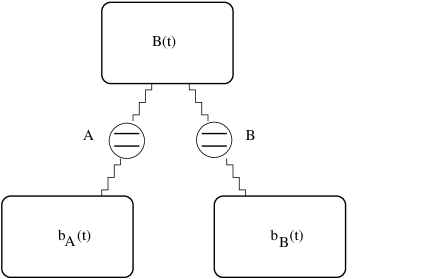
Figure 1: The model consists of two qubits A and B collectively interacting with the stochastic magnetic field $B(t)$ and separately interacting with the stochastic magnetic fields $b_{A}(t)$ and $b_{B}(t)$.

For simplicity, we assume that the stochastic fields $B(t),b_{A}(t),b_{B}(t)$ are classical and can be characterized as statistically independent Markov processes satisfying

$$<B(t)> = 0,$$ (4)

$$<B(t)B(t^{\prime})> = \frac{\Gamma}{\mu^{2}}\delta(t-t^{\prime}),$$ (5)

$$<b_{i}(t)> = 0,$$ (6)

$$<b_{i}(t)b_{i}(t^{\prime})> = \frac{\Gamma_{i}}{\mu^{2}}\delta(t-t^{\prime}),\,\,i=A,B$$ (7)

where $<...>$ stands for ensemble average. Here $\Gamma$ is the damping rate due to the collective interaction with $B(t)$, and $\Gamma_{i}$ are the damping rates of qubit $i$ $(i=A,B)$ due to the coupling to the fluctuating magnetic field $b_{i}(t)$. The white-noise properties in (5) and (7) ensure that the two-qubit system will undergo a Markov evolution. More realistic and more general models are easy to imagine, but for the sake of simplicity we will restrict ourselves to this simple situation.

Hamiltonian (1) represents a class of models of open quantum systems that describe a pure dephasing process, which can arise from interaction with Bosonic environments, independent of whether they are associated with quantized thermal radiation fields or phonon fields in solids or other specific physical contexts.

The dynamics under the Hamiltonian (1) can be described by a master equation, but for our purpose we find it more convenient to use the Kraus operator-sum representation (11). The advantage of the operator-sum representation will become clear in Sec. VI. The density matrix for the two qubits can be obtained by taking ensemble averages over the three noise fields $B(t),b_{A}(t),b_{B}(t)$:

$$\rho(t)=<<<\rho_{st}(t)>>>,$$ (8)

where the statistical density operator $\rho_{st}(t)$ is given by

$$\rho_{st}(t)=U(t)\rho(0)U^{\dagger}(t),$$ (9)

with the unitary operator

$$U(t)=\exp\left[-i\int^{t}_{0}dt^{\prime}H(t^{\prime})\right].$$ (10)

III Kraus representation for noisy channels

We can describe a decoherence process in the language of quantum channels wk . We take a quantum channel to be a completely positive linear map that acts on the quantum state space of a system of interest. Let ${\mathcal{E}}$ be a quantum channel that maps the input state $\rho_{\rm in}=\rho(0)$ into the output state $\rho_{\rm out}=\rho(t)$. It is known that the action of ${\mathcal{E}}$ can be characterized by a (not unique) set of operators called Kraus operators $K_{\mu}$ kra ; preskill ; mc . For any initial state, the action of quantum map ${\mathcal{E}}$ is given by

$$\rho(t)={\mathcal{E}}(\rho)=\sum_{\mu=1}^{N}K_{\mu}^{\dagger}(t)\rho(0)K_{\mu}(t),$$ (11)

where $K_{\mu}$ are Kraus operators satisfying

$$\sum_{\mu}K^{\dagger}_{\mu}K_{\mu}=I,$$ (12)

for all $t$. Eq. (11) is often termed the Kraus (or operator-sum) representation in the literature (for example, see preskill ; mc ). The operators $K_{\mu}$ contain all the information about the system’s dynamics. Unitary evolution is a special case with only one Kraus operator; otherwise the channel describes a non-unitary process associated with damping and decoherence. It can be easily seen that any $K_{\mu}$ projects pure states into pure states, but the collective action of different $K_{\mu}$’s will typically transform a pure state into a mixed state.

The most general solution (8) can be expressed in terms of twelve Kraus operators (under the assumption that the initial density matrix is not correlated with any of the three environments):

$$\rho(t)={\tilde{\mathcal{E}}}(\rho(0))=\sum^{2}_{i,j=1}\sum^{3}_{k=1}D_{k}^{\dagger}E^{\dagger}_{j}F^{\dagger}_{i}\rho(0)F_{i}E_{j}D_{k},$$ (13)

where the Kraus operators describing the interaction with the local environmental magnetic fields $b_{A}(t),b_{B}(t)$ are given by

$$E_{1}=\left(\begin{array}[]{clcr}1&&0\\ 0&&\gamma_{A}(t)\\ \end{array}\right)\otimes I,\,E_{2}=\left(\begin{array}[]{clcr}0&\,\,\,\,0\\ 0&\,\,\,\omega_{A}(t)\\ \end{array}\right)\otimes I,\,\,$$ (18)

$$F_{1}=I\otimes\left(\begin{array}[]{clcr}1&\,\,\,0\\ 0&\,\,\,\gamma_{B}(t)\\ \end{array}\right),\,F_{2}=I\otimes\left(\begin{array}[]{clcr}0&\,\,\,0\\ 0&\,\,\,\omega_{B}(t)\\ \end{array}\right),\,\,$$ (23)

and the Kraus operators that describe the collective interaction with the environmental magnetic field $B(t)$ are given by

$$D_{1}=\begin{pmatrix}\gamma(t)&0&0&0\\ 0&1&0&0\\ 0&0&1&0\\ 0&0&0&\gamma(t)\end{pmatrix},$$ (24)

$$D_{2}=\begin{pmatrix}\omega_{1}(t)&0&0&0\\ 0&0&0&0\\ 0&0&0&0\\ 0&0&0&\omega_{2}(t)\end{pmatrix},$$ (25)

$$D_{3}=\begin{pmatrix}0&0&0&0\\ 0&0&0&0\\ 0&0&0&0\\ 0&0&0&\omega_{3}(t)\end{pmatrix},$$ (26)

Note that the parameters appearing in (18)–(26) are given by

$$\gamma_{A}(t) = {e}^{-{t}/{2T^{A}_{2}}},\,\,\,\gamma_{B}(t)={e}^{-{t}/{2T^{B}_{2}}},$$ (27)

$$\omega_{A}(t) = \sqrt{1-e^{-{t}/{T^{A}_{2}}}},\,\,\omega_{B}(t)=\sqrt{1-e^{-{t}/{T^{B}_{2}}}},$$ (28)

$$\gamma(t) = e^{-t/2T_{2}},\,\,\omega_{1}(t)=\sqrt{1-e^{-t/T_{2}}},$$ (29)

$$\omega_{2}(t) = -e^{-t/T_{2}}\sqrt{1-e^{-t/T_{2}}},$$ (30)

$$\omega_{3}(t) = \sqrt{(1-e^{-t/T_{2}})(1-e^{-2t/T_{2}})},$$ (31)

where $T_{2}=1/\Gamma$ is the phase relaxation time due to the collective interaction with $B(t)$ and $T^{A}_{2}=1/\Gamma_{A}$ and $T^{B}_{2}=1/\Gamma_{B}$ are the phase relaxation times for qubit A and qubit B due to the interaction with their own environments $b_{A}(t),b_{B}(t)$, respectively. We will no longer write the time-dependent arguments of the $\gamma$’s and $\omega$’s as a notational simplification.

IV Explicit Solutions, Various Density Matrices

Three cases can be distinguished: (1) The case that the two qubits only interact with their local environments, namely $B(t)=0$; and (2) the case in which only one qubit is affected by a local environment, that is, $B(t)=0$ and one of $b_{A}(t),b_{B}(t)$ is also zero. We call the above two cases the two-qubits local dephasing channel and the one-qubit local dephasing channel, respectively. (3) The case that the two qubits only collectively interact with $B(t)$. We call this case the collective dephasing channel. We will present these three cases separately in what follows.

IV.1 Two-qubit local dephasing channel ${\mathcal{E}}_{AB}$

When the pair of qubits only interact with the local magnetic fields, i.e. $B(t)=0$, then the phase-noisy channel, denoted by ${\mathcal{E}}_{AB}$, is characterized by the following four composite Kraus operators:

$$M_{1} = E_{1}F_{1},\,\,\,M_{2}=E_{1}F_{2},\,\,\,$$ (32)

$$M_{3} = E_{2}F_{1},\,\,\,M_{4}=E_{2}F_{2},$$ (33)

where the fundamental Kraus operators $E_{1},E_{2},F_{1},F_{2}$ are defined in (18), and (23). Therefore, the effect of the quantum channel ${\mathcal{E}}_{AB}$ on an initial state $\rho$ can be described as follows:

$$\rho(t)={\mathcal{E}}_{AB}(\rho(0))=\sum_{\mu=1}^{4}M_{\mu}^{\dagger}\rho(0)M_{\mu}.$$ (34)

The explicit solution in the standard basis is given by

$$\rho(t)={\mathcal{E}}_{AB}(\rho(0))$$

$$=\begin{pmatrix}\rho_{11}&\gamma_{B}\rho_{12}&\gamma_{A}\rho_{13}&\gamma_{A}\gamma_{B}\rho_{14}\\ \gamma_{B}\rho_{21}&\rho_{22}&\gamma_{A}\gamma_{B}\rho_{23}&\gamma_{A}\rho_{24}\\ \gamma_{A}\rho_{31}&\gamma_{A}\gamma_{B}\rho_{32}&\rho_{33}&\gamma_{B}\rho_{34}\\ \gamma_{A}\gamma_{B}\rho_{41}&\gamma_{A}\rho_{42}&\gamma_{B}\rho_{43}&\rho_{44}\end{pmatrix}.$$ (35)

where $\gamma_{A}$ and $\gamma_{B}$ are defined in (27) and the notation $\rho_{ij}$ stands for the initial state $\rho_{ij}(0)$

One immediate conclusion that can be drawn from Eq. (IV.1) is that the two-qubit dephasing channel has an effect on all the matrix elements except for the diagonal elements. Thus, decoherence takes place in every superposed state of the basis elements (II). Furthermore, it will turn out later in Sec. VI that this channel generally results in faster disentanglement.

IV.2 One-qubit local dephasing channels ${\mathcal{E}}_{A}$ and ${\mathcal{E}}_{B}$

A simple case arises if the channel is assumed to affect only one qubit, say qubit A. In this situation, we call the channel a one-qubit local dephasing channel, and denote it by ${\mathcal{E}}_{A}$. The one-qubit dephasing channel ${\mathcal{E}}_{A}$ can be described by the Kraus operators $E_{1},E_{2}$. Explicitly, for any initial state $\rho(0)$, the output state under this channel is given by

$$\rho(t) = {\mathcal{E}}_{A}(\rho(0))=\sum_{\mu=1}^{2}E_{\mu}^{\dagger}\rho(0)E_{\mu}$$ (36)

$$= \begin{pmatrix}\rho_{11}&\rho_{12}&\gamma_{A}\rho_{13}&\gamma_{A}\rho_{14}\\ \rho_{21}&\rho_{22}&\gamma_{A}\rho_{23}&\gamma_{A}\rho_{24}\\ \gamma_{A}\rho_{31}&\gamma_{A}\rho_{32}&\rho_{33}&\rho_{34}\\ \gamma_{A}\rho_{41}&\gamma_{A}\rho_{42}&\rho_{43}&\rho_{44}\end{pmatrix}.$$

Obviously, one can equally well define in terms of Kraus operators $F_{1},F_{2}$ the one-qubit local dephasing channel ${\mathcal{E}}_{B}$, that has effect only on qubit B.

Since the one-qubit dephasing channels only affect a single qubit, the coherence of the other qubit is not affected during processing. Consequently, the coherence of the composite two-qubit system cannot be destroyed completely. The details of the loss of coherence and entanglement under the channels defined above will be given in Sec. V and Sec. VI.

IV.3 Collective dephasing channel ${\mathcal{E}}_{D}$

If the local stochastic fields $b_{A}(t),b_{B}(t)$ are negligible or switched off, we obtain a model that describes the two qubits collectively interacting with a common environment ye ; braun . In this case, the solution $\rho(t)$ can be cast into the operator-sum representation in terms of the three Kraus operators $D_{\mu}$:

$$\rho(t)={\mathcal{E}}_{D}(\rho(0))=\sum_{\mu=1}^{3}D^{\dagger}_{\mu}(t)\rho(0)D_{\mu}(t),$$ (37)

where $D_{\mu},\,\,(\mu=1,2,3)$ are given in (24),  (25) and (26).

The explicit solution of (37) in the standard basis (II) can then be expressed as

$$\rho(t) = {\mathcal{E}}_{D}(\rho(0))$$ (38)

$$= \begin{pmatrix}\rho_{11}&\gamma\rho_{12}&\gamma\rho_{13}&\gamma^{4}\rho_{14}\\ \gamma\rho_{21}&\rho_{22}&\rho_{23}&\gamma\rho_{24}\\ \gamma\rho_{31}&\rho_{32}&\rho_{33}&\gamma\rho_{34}\\ \gamma^{4}\rho_{41}&\gamma\rho_{42}&\gamma\rho_{43}&\rho_{44}\end{pmatrix},$$

where $\gamma=e^{-t/2T_{2}}$ is defined in (29).

As seen from (38), the collective dephasing channel affects the off-diagonal elements $\rho_{14},\rho_{41}$ more severely than it affects the other off-diagonal elements. As a result, we have already shown in ye that, for a set of entangled pure states containing $\rho_{14},\rho_{41}$, disentanglement proceeds with rates that are faster than the dephasing rates for qubit A or qubit B. In the case of collective coupling, the stochastic magnetic field $B(t)$ always affects the phases of qubit A and qubit B in the same way, so one expects that for some states the random phases may cancel each other out. Here such a cancellation due to the underlying symmetry of the interaction Hamiltonian can be expected and has been demonstrated in various contexts decohfree . For the situation considered here, the cancellation leads to the existence of the disentanglement-free subspaces spanned by a basis consisting of $|2\rangle_{AB},\,\,|3\rangle_{AB}$. The entangled states belonging to these subspaces are robust entangled states ye .

V Local dephasing and mixed dephasing

First, we study the coherence decay of a single qubit under the two-qubit dephasing channel ${\mathcal{E}}_{AB}$ defined in (IV.1). The local dephasing rate of the qubit can be determined from the reduced density matrices $s^{A}$ and $s^{B}$, obtained from the density matrix (IV.1) in the usual way, that is,

$$s^{A}\equiv{\rm Tr}_{B}\{\rho\}\quad{\rm and}\quad s^{B}\equiv{\rm Tr}_{A}\{\rho\}.$$ (39)

The reduced density matrices for qubit A and qubit B are thus obtained as:

$$s^{A}(t)=\begin{pmatrix}\rho_{11}(t)+\rho_{22}(t)\,\,&\,\,\rho_{13}(t)+\rho_{24}(t)\\ &\\ \rho_{31}(t)+\rho_{42}(t)\,\,&\,\,\rho_{33}(t)+\rho_{44}(t)\end{pmatrix},$$ (40)

and

$$s^{B}(t)=\begin{pmatrix}\rho_{11}(t)+\rho_{33}(t)\,\,&\,\,\rho_{12}(t)+\rho_{34}(t)\\ \rho_{21}(t)+\rho_{43}(t)\,\,&\,\,\rho_{22}(t)+\rho_{44}(t)\end{pmatrix}\quad.$$ (41)

The dephasing rates are determined by the off-diagonal elements:

$$s^{A}_{12}(t)=\rho_{13}(t)+\rho_{24}(t)=\gamma_{A}s^{A}_{12}(0),$$ (42)

and

$$s^{B}_{12}(t)=\rho_{12}(t)+\rho_{34}(t)=\gamma_{B}s^{B}_{12}(0).$$ (43)

Thus, the dephasing times denoted by $\tau_{A,B}$ for qubits A and B, respectively, can be read off from the expressions for $\gamma_{A}$ and $\gamma_{B}$. That is

$$\tau_{A}\equiv\frac{2}{\Gamma_{A}},\quad{\rm and}\quad\tau_{B}\equiv\frac{2}{\Gamma_{B}}.$$ (44)

Similar to local dephasing processes, the decoherence rate for the composite two-qubit system is characterized by the decay rates of the off-diagonal elements of the density matrix (IV.1). As seen from (IV.1), the two-qubit off-diagonal elements $\rho_{ij}(i<j)$, are given by

$$\rho_{ij}(t)=e^{-\Gamma_{ij}t}\rho_{ij}(0)$$ (45)

so the coherence $\rho_{ij}(t)$ decays on a timescale

$$\tau_{\rm dec}=\frac{1}{\Gamma_{ij}},$$ (46)

where $\Gamma_{12}=\Gamma_{34}=\Gamma_{B}/2,\Gamma_{13}=\Gamma_{24}=\Gamma_{A}/2,\Gamma_{14}=\Gamma_{23}=(\Gamma_{A}+\Gamma_{B})/2.$

We denote $\tau$ as a time scale on which all the off-diagonal elements of the density matrix (IV.1) disappear. The corresponding decoherence rate $1/\tau$ is called here the mixed dephasing rate in order to distinguish it from the local dephasing rates of a single qubit. It is evident that the mixed dephasing rate $1/\tau$ is determined by the slower decaying elements com , and in general, we have,

$$\tau\geq\tau_{A},\tau_{B}.$$ (47)

Namely, and this is a key point, the mixed dephasing rate $1/\tau$ is not shorter than the local dephasing rates for qubit A or qubit B defined in (44). As will be seen in the next section, this is in contrast with the disentanglement rate, which can be faster than the local rates $1/\tau_{A}$ and $1/\tau_{B}$.

Finally, we study dephasing processes under the local one-qubit dephasing channels ${\mathcal{E}}_{A}$ and ${\mathcal{E}}_{B}$. Since the local dephasing channels only affect one qubit and leave the other intact, hence some coherence may always exist in the composite two-qubit state. Let us consider the channel ${\mathcal{E}}_{A}$ and a superposed state of just three members of the standard basis,

$$|\psi\rangle_{AB}=\frac{1}{\sqrt{3}}\Big{(}|1\rangle_{AB}+|2\rangle_{AB}+|4\rangle_{AB}\Big{)}.$$ (48)

Obviously, from (36), we see there is no way that the channel ${\mathcal{E}}_{A}$ can destroy the off-diagonal elements $\rho_{12},\rho_{21}$, so ${\mathcal{E}}_{A}$ cannot completely destroy the coherence of the composite two-qubit state (48). Next, we look at the dephasing processes for an individual qubit. Obviously, the coherence of qubit B is not affected by ${\mathcal{E}}_{A}$. That is,

$$s^{B}(t)=s^{B}(0).$$ (49)

Notice that $s^{A}(t)$ under the channel ${\mathcal{E}}_{A}$ is given by (40). Hence, as expected, the coherence of qubit A will be destroyed by the channel ${\mathcal{E}}_{A}$ on the dephasing time scale $\tau_{A}$. A similar analysis applies to ${\mathcal{E}}_{B}$.

VI Entanglement decay

To describe the temporal evolution of quantum entanglement we have to measure the amount of entanglement contained in a quantum state. Since the entanglement decoherence processes are typically associated with mixed states, we will use Wootter’s concurrence to quantify the degree of entanglement woo . The concurrence varies from $C=0$ for a disentangled state to $C=1$ for a maximally entangled state. For two qubits, the concurrence may be calculated explicitly woo from the density matrix $\rho$ for qubits A and B:

$$C(\rho)=\max\left(0,\sqrt{\lambda_{1}}-\sqrt{\lambda_{2}}-\sqrt{\lambda_{3}}-\sqrt{\lambda_{4}}\,\,\right),$$ (50)

where the quantities $\lambda_{i}$ are the eigenvalues of the matrix

$$\varrho=\rho(\sigma^{A}_{y}\otimes\sigma^{B}_{y})\rho^{*}(\sigma^{A}_{y}\otimes\sigma^{B}_{y}),$$ (51)

arranged in decreasing order. Here $\rho^{*}$ denotes the complex conjugation of $\rho$ in the standard basis (II) and $\sigma_{y}$ is the Pauli matrix expressed in the same basis as:

$$\sigma^{A,B}_{y}=\begin{pmatrix}0\,\,&\,\,\,-i\\ i\,\,&\,\,\,\,0\end{pmatrix}.$$ (52)

For a pure state $|\psi\rangle$, the concurrence (50) is reduced to

$$C(|\psi\rangle)=|\langle\psi|\sigma_{y}^{A}\otimes\sigma_{y}^{B}|\psi^{*}\rangle|.$$ (53)

VI.1 Entanglement decay under two-qubit dephasing channel ${\mathcal{E}}_{AB}$

How does the concurrence behave under a noisy channel? From (53), for any entangled pure state

$$|\Psi\rangle=a_{1}|1\rangle_{AB}+a_{2}|2\rangle_{AB}+a_{3}|3\rangle_{AB}+a_{4}|4\rangle_{AB},$$ (54)

where $\sum_{i=1}^{4}|a_{i}|^{2}=1$, the concurrence of the pure state (54) is given by

$$C(|\Psi\rangle)=2|a_{1}a_{4}-a_{2}a_{3}|.$$ (55)

It follows from (IV.1) that the concurrence (55) will always decay to zero on a time scale determined by the dephasing time $\tau$ defined in (47). In fact, let us first note that the density matrix of (54) will approach a diagonal matrix at the two-qubit dephasing rate $1/\tau$. Since a diagonal density matrix only describes classical probability, then the concurrence must be zero.

Moreover, we show in what follows that all entangled (possibly mixed) states decay at rates that are faster than the dephasing rates of an individual qubit. For this purpose, we first note that the concurrence $C(\rho)$ is a convex function of $\rho$ woo ; that is, for any positive numbers $p_{\mu}$ and density matrices $\rho_{\mu}$, $(\mu=1,..,n)$ such that $\sum_{\mu}p_{\mu}=1$, one has

$$C\Big{(}\sum_{\mu=1}^{n}p_{\mu}\rho_{\mu}\Big{)}\leq\sum_{\mu=1}^{n}p_{\mu}C(\rho_{\mu}).$$ (56)

Applying the above inequality to (IV.1), we immediately get

$$C(\rho(t))\leq\sum_{\mu=1}^{4}C(M_{\mu}^{\dagger}\rho(0)M_{\mu}),$$ (57)

where $M_{\mu}$ are defined in (32) and (33). Now we consider a typical term $C(M_{\mu}^{\dagger}\rho(0)M_{\mu})$ in (57) and denote it by

$$\rho_{\rm out}=M_{\mu}^{\dagger}\rho(0)M_{\mu}.$$ (58)

Substituting (58) into (51), we have,

$$\varrho = \rho_{\rm out}(\sigma^{A}_{y}\otimes\sigma^{B}_{y})\rho_{\rm out}^{*}(\sigma^{A}_{y}\otimes\sigma^{B}_{y})$$ (59)

$$= M_{\mu}^{\dagger}\rho M_{\mu}(\sigma^{A}_{y}\otimes\sigma^{B}_{y})M^{T}_{\mu}\rho^{*}M_{\mu}(\sigma^{A}_{y}\otimes\sigma^{B}_{y}).$$ (60)

Notice that $\varrho$ has the same eigenvalues as $\varrho^{\prime}$

$$\varrho^{\prime}=\rho M_{\mu}(\sigma^{A}_{y}\otimes\sigma^{B}_{y})M_{\mu}^{T}\rho^{*}M^{*}_{\mu}(\sigma^{A}_{y}\otimes\sigma^{B}_{y})M_{\mu}^{\dagger}.$$ (61)

Also note that the Kraus operators defined in (18) satisfy $M^{T}_{\mu}=M_{\mu}^{\dagger}=M_{\mu}^{*}$. Hence it is easy to check that

$$M_{\mu}(\sigma^{A}_{y}\otimes\sigma_{y}^{B})M_{\mu}=\left\{\begin{array}[]{ll}\gamma_{A}\gamma_{B}(\sigma^{A}_{y}\otimes\sigma^{B}_{y})&\mbox{if $\mu=1$ },\\ 0&\mbox{if $\mu\neq 1$}.\end{array}\right.$$ (62)

Then Eq. (61) becomes:

$$\varrho^{\prime\prime}=\left\{\begin{array}[]{ll}\gamma^{2}_{A}\gamma_{B}^{2}\rho(\sigma^{A}_{y}\otimes\sigma^{B}_{y})\rho^{*}(\sigma^{A}_{y}\otimes\sigma^{B}_{y})&\mbox{if $\mu=1$},\\ 0&\mbox{if $\mu\neq 1$}.\end{array}\right.$$ (63)

By using the definition of concurrence (51) and the inequality (57), we get:

$$C(\rho(t))\leq\gamma_{A}\gamma_{B}C(\rho(0)).$$ (64)

Hence, the entanglement decay time $\tau_{e}$ can be identified as

$$\frac{1}{\tau_{e}}=\frac{1}{\tau_{A}}+\frac{1}{\tau_{B}},$$ (65)

where the local dephasing times $\tau_{A},\tau_{B}$ are given in (44). In this way we immediately see that the entanglement decay times for the two-qubit channel are shorter than the local dephasing times $\tau_{A},\tau_{B}$ and hence are shorter than the mixed dephasing time $\tau$ as well.

By suitably choosing the channel parameters $\Gamma_{A},\Gamma_{B}$, one can achieve

$$\tau_{e}\ll\tau,$$ (66)

where $\tau$ is the mixed dephasing time (47). We have shown here that the decay time for the entanglement of the two-qubit system can be much shorter than the mixed dephasing time $\tau$. An interesting case occurs when the phasing damping rates for qubit A and qubit B are assumed the same: $\tau_{A}=\tau_{B}$, then from (65), we have

$$\tau_{e}=\frac{\tau_{A}}{2}=\frac{\tau_{B}}{2}=\frac{\tau}{2}.$$ (67)

This relation reminds us of the well-known relation between the phase coherence relaxation rate $T_{2}$ and the diagonal element decay rate $T_{1}$ in open quantum systems open .

To see how the phase-noisy channels affect entanglement in a more explicit way, it would be instructive to find some examples in which the concurrence can explicitly be calculated. For this purpose, let us consider, for example, the following two classes of almost arbitrary bipartite pure states described by:

$$|\phi_{1}\rangle = a_{1}|1\rangle_{AB}+a_{2}|2\rangle_{AB}+a_{4}|4\rangle_{AB},$$ (68)

$$|\phi_{2}\rangle = a_{1}|1\rangle_{AB}+a_{3}|3\rangle_{AB}+a_{4}|3\rangle_{AB},$$ (69)

and

$$|\psi_{1}\rangle = a_{1}|1\rangle_{AB}+a_{2}|2\rangle_{AB}+a_{3}|3\rangle_{AB},$$ (70)

$$|\psi_{2}\rangle = a_{2}|2\rangle_{AB}+a_{3}|3\rangle_{AB}+a_{4}|4\rangle_{AB}.$$ (71)

It will turn out in what follows that the concurrence for those two classes can be calculated exactly.

For the pure state (68), the concurrence is $C(|\phi_{1}\rangle)=2|a_{1}a_{4}|$. Then the density matrix with the initial entangled state (68) at $t$ is given by

$$\rho(t) = {\mathcal{E}}_{AB}(\rho)$$ (72)

$$= \begin{pmatrix}|a_{1}|^{2}&\gamma_{B}a_{1}a_{2}^{*}&0&\gamma_{A}\gamma_{B}a_{1}a_{4}^{*}\\ \gamma_{B}a_{2}a_{1}^{*}&|a_{2}|^{2}&0&\gamma_{A}a_{2}a_{4}^{*}\\ 0&0&0&0\\ \gamma_{A}\gamma_{B}a_{4}a_{1}^{*}&\gamma_{A}a_{4}a_{2}^{*}&0&|a_{4}|^{2}\end{pmatrix}.$$

The non-zero eigenvalues of the matrix $\varrho$ defined in (51) are

$$\lambda_{1}=(1+\gamma_{A}\gamma_{B})^{2}|a_{1}a_{4}|^{2},\,\,\,\lambda_{2}=(1-\gamma_{A}\gamma_{B})^{2}|a_{1}a_{4}|^{2}.$$ (73)

Then the concurrence at $t$ is given by

$$C(\rho(t))=2\gamma_{A}\gamma_{B}|a_{1}a_{4}|.$$ (74)

Similarly, as another illustration, we may calculate the entanglement degree of the entangled states (70). The density matrix with the initial entangled state (70) at $t$ is given by

$$\rho(t) = {\mathcal{E}}_{AB}(\rho)$$ (75)

$$= \begin{pmatrix}|a_{1}|^{2}&\gamma_{B}a_{1}a_{2}^{*}&\gamma_{A}a_{1}a_{3}^{*}&0\\ \gamma_{B}a_{2}a_{1}^{*}&|a_{2}|^{2}&\gamma_{A}\gamma_{B}a_{2}a_{3}^{*}&0\\ \gamma_{A}a_{3}a_{1}^{*}&\gamma_{A}\gamma_{B}a_{3}a_{2}^{*}&|a_{3}|^{2}&0\\ 0&0&0&0\end{pmatrix}.$$

The concurrence at $t$ can be obtained

$$C(\rho(t))=2\gamma_{A}\gamma_{B}|a_{2}a_{3}|.$$ (76)

From the above two examples, we see that the concurrence is determined by the fast decaying off-diagonal elements $\rho_{14}$ and $\rho_{23}$. The examples also demonstrate that the bound in (64) is the minimal upper bound.

VI.2 Entanglement decay under one-qubit dephasing channels ${\mathcal{E}}_{A}$ or ${\mathcal{E}}_{B}$

Perhaps the best way of seeing the difference between the disentanglement and decoherence is to look at the effect of the one-qubit channel on a two-qubit system. Similar to the two-qubit dephasing channels, it can be shown that under the one-qubit local dephasing channels, the concurrence is determined as follows:

$$C({\mathcal{E}}_{A}(\rho(0)) \leq \gamma_{A}C(\rho(0)),$$ (77)

$$C({\mathcal{E}}_{B}(\rho(0)) \leq \gamma_{B}C(\rho(0)).$$ (78)

Thus, we see that the one-qubit local dephasing channels can completely destroy the quantum entanglement after the dephasing times $\tau_{A}$ or $\tau_{B}$ . To be more specific, let us consider the following entangled pure state:

$$|\phi\rangle=\frac{1}{\sqrt{3}}\Big{(}|1\rangle_{AB}+|3\rangle_{AB}+|4\rangle_{AB}\Big{)}.$$ (79)

If we apply the local dephasing channel ${\mathcal{E}}_{A}$ on $\rho=|\phi\rangle\langle\phi|$ then the output state is given by

$$\rho(t) = {\mathcal{E}}_{A}(\rho)$$ (80)

$$= \begin{pmatrix}\frac{1}{3}&0&\frac{\gamma_{A}}{3}&\frac{\gamma_{A}}{3}\\ 0&0&0&0\\ \frac{\gamma_{A}}{3}&0&\frac{1}{3}&\frac{1}{3}\\ \frac{\gamma_{A}}{3}&0&\frac{1}{3}&\frac{1}{3}\end{pmatrix}.$$

The concurrence of (80) can be obtained

$$C(\rho(t))=\frac{2}{3}e^{-t/2T^{A}_{2}}.$$ (81)

This means that disentanglement will proceed exponentially in the local dephasing time $\tau_{A}$. As seen from Sec. V, however, the coherence of the composite two-qubit state $|\phi\rangle$ cannot be destroyed completely. In general, one-qubit local dephasing channels ${\mathcal{E}}_{A}$ and ${\mathcal{E}}_{B}$ cannot destroy the coherence between different elements of the basis (54). That is

$$\rho(t)\neq\sum_{i=1}^{4}|a_{i}|^{2}|i\rangle\langle i|,\,\,\,{\rm as}\,\,t\rightarrow\infty.$$ (82)

Namely, the decoherence process for the composite two-qubit system becomes frozen after the local dephasing times $\tau_{A}$ or $\tau_{B}$.

In summary, we have shown that the effect of the dephasing channels on entanglement and quantum coherence may differ substantially. In general, the entanglement of two qubits decays faster than the quantum coherence. In particular, for the channels ${\mathcal{E}}_{A}$ and ${\mathcal{E}}_{B}$, we have shown that for some entangled states the local dephasing channels cannot completely destroy the coherence between the qubits. However, entanglement as a global property can be completely destroyed by the one-qubit local dephasing channels.

VII Input-output fidelity and concurrence

It is interesting to look at the coherence and entanglement decays by comparing input-output fidelity and concurrence. The fidelity is meant to measure the “difference” between an input state and an output state under a noisy quantum channel. As such, it has been used to measure the loss of coherence of a quantum state when the state is subject to the influence of an environment. The fidelity can be defined as

$$F(\rho_{\rm in},\rho_{\rm out})=\max|\langle\psi_{1}|\psi_{2}\rangle|,$$ (83)

where the maximum is taken over all purifications $|\psi_{1}\rangle,$ $|\psi_{2}\rangle$ of $\rho_{\rm in}$ and $\rho_{\rm out}$ jo ; shu . For a pure initial state $\rho_{\rm in}=|\psi\rangle\langle\psi|,$ it can simply be written as

$$F(\rho_{\rm in},\rho_{\rm out})=\langle\psi|\rho_{\rm out}|\psi\rangle.$$ (84)

In the case of the one-qubit dephasing channel ${\mathcal{E}}_{A}$ defined in (36), for the general entangled states (54), Eq. (84) can be written as

$$F(\rho,{\mathcal{E}}_{A}(\rho)) = \sum_{i=1}^{4}|a_{i}|^{4}$$ (85)

$$+ 2\gamma_{A}\left(|a_{1}a_{4}|^{2}+|a_{2}a_{3}|^{2}\right)$$

$$+ 2\gamma_{A}\left(|a_{1}a_{3}|^{2}+|a_{2}a_{4}|^{2}\right)$$

$$+ 2\left(|a_{1}a_{2}|^{2}+|a_{3}a_{4}|^{2}\right).$$

For example, we consider the entangled pure state (54) with coefficients

$$a_{1}=a_{2}=a_{3}={\frac{1}{2}},\,\,a_{4}=-{\frac{1}{2}}.$$ (86)

Then it is easy to check that, for all times $t$, one has

$$F(\rho,{\mathcal{E}}_{A}(\rho))\geq\frac{1}{2}.$$ (87)

Hence we again see that some amount of coherence is always preserved. However, as shown in the previous discussions, it is obvious that the disentanglement will be complete; that is, $C$ decays to zero on the scale of the local dephasing time $\tau_{A}$:

$$C(\rho)=1,\,\,C({\mathcal{E}}_{A}(\rho))=0.$$ (88)

VIII Concluding remarks

In this last section we provide some comments on disentanglement, mixed dephasing processes, and local dephasing processes for an individual qubit.

It is evident from sections V and VI that in general entanglement is more fragile than local quantum coherence. In the case of the examples (74) and (76), we see that quantum entanglement is determined by the off-diagonal elements $\rho_{14},\rho_{23}$ and their conjugates. In our two-qubit model, these elements are affected more severely than other off-diagonal elements. So the disentanglement normally proceeds in a rate which is faster than the dephasing rate, the latter being generally determined by the slow-changing off-diagonal elements $\rho_{12},\rho_{13}$ etc.

We remark that our simple approach to decoherence in terms of phase damping channels can easily be extended to other decoherence channels such as amplitude damping channels. Although the disentanglement rates are dependent on the choice of the measure of entanglement, it seems that the fast disentanglement demonstrated in the paper is of generic character.

Since the local manipulations of a single qubit cannot increase the entanglement between two qubits, so the quantum map (IV.1) cannot create any entanglement. This is in contrast to the collective dephasing channel ${\mathcal{E}}_{D}$. It is known that entanglement may be created due to the interaction with a common heat bath braun .

In connection to the foundations of quantum theory, a good understanding of entanglement decoherence might provide a more detailed picture of the transition from quantum to classical (or semiclassical) dynamics. As suggested in this paper, a quantum system with several constituent particles, if initially in an entangled state, may undergo several stages of transition, including the “collapse” of entanglement, and then the “collapse” of coherence among individual particles. This is a topic to be addressed in future publications.

Summarizing, our primary interest in this paper is to investigate the fragility of quantum entanglement. Through simple two-qubit systems we have shown that the most commonly assumed (dephasing) model of noisy environments may affect entanglement and quantum coherence in a very different manner. While preserved in the case of collective interaction, the permutation symmetry of the two qubits is violated by local environment interactions. As a result, there are no entanglement decoherence-free subspaces for the local dephasing models, which means that entanglement for all entangled states will decay into zero after some time. Our results suggest that, when spins are coupled to inhomogeneous external magnetic fields, disentanglement and dephasing may proceed in rather different time scales. It means that, even in the situation that quantum coherence has relatively long relaxation times, entanglement may be rapidly suppressed. This issue is certainly of importance in realizing qubits as spins of electrons or nuclei in solids.

References

- (1) W. H. Zurek, Phys. Today 44 (10), 36 (1991); Phys. Rev. D 24, 1516 (1981); 26, 1862 (1982); Prog. Theor. Phys. 89, 281 (1993).
- (2) E. Joos and H. D. Zeh, Z. Phys. B 59, 223 (1985).
- (3) D. Braun, F. Haake, and W. T. Strunz, Phys. Rev. Lett. 86, 2913(2001); W. T. Strunz, F. Haake, and D. Braun, Phys. Rev. A 67, 022101 (2003); W. T. Strunz and F. Haake, Phys. Rev. A 67, 022102 (2003).
- (4) C. H. Bennett and G. Brassard, Proceedings of the IEEE conference on computers, Systems, and Signal Processing, Bangalore, 1984 (IEEE, New York, 1984), P.175.
- (5) A. K. Ekert, Phys. Rev. Lett. 67, 661 (1991).
- (6) A. Muller, H. Zbinden, N. Gisin, Europhys. Lett. 33, 335 (1996).
- (7) C. H. Bennett, G. Brassard, C. Crépeau, R. Jozsa, A. Peres, and W. K. Wooters, Phys. Rev. Lett. 69, 1895(1993).
- (8) C. H. Bennett and S. J. Wiesner, Phys. Rev. Lett. 69, 2881 (1992).
- (9) D. Deutsch and R. Josza, Proc. R. Soc. London A. 439, 553 (1992).
- (10) P. W. Shor, SIAM J. Comp. 26 (5), 1484 (1997).
-
(11)
J. Preskill, Lecture Notes on Quantum
Information and Quantum Computation
at www.theory.caltech.edupeoplepreskillph229. - (12) M. A. Nielson and I. L. Chuang, Quantum Computation and Quantum Information (Cambridge, England, 2000).
- (13) J. I. Cirac and P. Zoller, Nature (London) 404, 579 (2000); J. I. Cirac and P. Zoller, Phys. Rev. Lett. 74, 4091 (1995).
- (14) D. Kielpinski, C. Monroe and D. J. Wineland, Nature 417, 709 (2002); D. Kielpinski, V. Meyer, M. A. Rowe, C. A. Sackett, W. M. Itano, C. Monroe and D. J. Wineland, Science 291, 1013 (2001).
- (15) P. W. Shor, Phys. Rev. A 52, 2493 (1995).
- (16) A. Steane, Phys. Rev. Lett. 77, 793 (1996).
- (17) R. Laflamme, C. Miquel, J. P. Paz, and W. H. Zurek, Phys. Rev. Lett. 77, 198 (1996).
- (18) G. M. Palma, K.-A. Suominen and A. K. Ekert, Proc. R. Soc. London A 452, 557 (1996).
- (19) P. Zanardi and M. Rasetti, Phys. Rev. Lett. 79, 3306 (1997).
- (20) L.-M. Duan and G.-C. Guo, Phys. Rev. A 57, 2399 (1998).
- (21) D. A. Lidar and I. L. Chuang and K. B Whaley, Phys. Rev. Lett. 81, 2594 (1998).
- (22) A. Beige, D. Braun, B. Tregenna and P. L. Knight, Phys. Rev. Lett. 85, 1762 (2000).
- (23) L. Viola, E. M. Fortunato, M. A. Pravia, E. Knill, R. Laflamme and D. G. Gory, Science 293, 2059 (2001).
- (24) L. Viola, E. Knill, and S. Lloyd, Phys. Rev. Lett. 83, 4888 (1999).
- (25) M. Horodecki, P. Horodecki and R. Horodecki, in Quantum Information: An Introduction to Basic Theoretical Concepts and Experiments, edited by G. Alber, Springer Tracts in Modern Physics Vol. 173 (Springer-Verlag, Berlin, 2001).
- (26) N. Gisin, Phys Lett A 210, 151 (1996) and references therein.
- (27) V. Vedral, M. B. Plenio, M. A. Rippin, and P. L. Knight, Phys. Rev. Lett. 78, 2275 (1997).
- (28) F. Verstrate and M. M. Wolf, Phys. Rev. Lett. 89, 170401 (2002)
- (29) S. Virmani and M. B. Plenio, quant-ph/0212020 (unpublished).
- (30) S. Hill and W. K. Wootters, Phys. Rev. Lett. 78, 5022 (1997); W. K. Wootters, Phys. Rev. Lett. 80, 2245 (1998).
- (31) T. Yu and J. H. Eberly, Phys. Rev. B 66, 193306 (2002), quant-ph/0209037.
- (32) D. Braun, Phys. Rev. Lett. 89, 277901 (2003).
- (33) Natural and induced symmetries can be cited as the source of “protection” from decoherence in a variety of contexts. Examples are found in (i) two-atom spontaneous emission: G. S. Agarwal, Quantum Statistical Theories of Spontaneous Emission and their Relation to Other Approaches, Springer Tracts in Modern Physics Vol. 70 (Springer-Verlag, Berlin, 1974), sec. 11, (ii) at a confluence of coherences: K. Rzazewski and J.H. Eberly, Phys. Rev. Lett. 47, 408 (1980), (iii) in connection with laser-induced continuum structures (LICS): P.L. Knight, M.A. Lauder and B.J. Dalton, Phys. Rep. 190, 1 (1990), and (iv) in more recent quantum information settings: See the review paper, D. A. Lidar and K. B. Whaley, quant-ph/0301032 (2003) and additional references therein.
- (34) K. Wódkiewicz, Opt. Express 8, No. 2, 145 (2001); S. Daffer, K. Wódkiewicz, and J. McIver, quant-ph/0211001 (unpublished).
- (35) K. Kraus, States, Effect, and Operations: Fundamental Notions in Quantum Theory (Springer-Verlag, Berlin, 1983).
- (36) Obviously, there exist some special entangled states, such as the Bell states and , where the dephasing rates are determined by terms appearing in (IV.1). Throughout the paper, we will be interested in more general cases.
- (37) See, for example, L. Allen and J. H. Eberly, Optical Resonance and Two-Level Atoms, (Dover, New York, 1987).
- (38) R. Jozsa, J. Mod. Opt. 41, 2315 (1994).
- (39) B. Schumacher, Phys. Rev. A 54, 2614 (1996); B. Schumacher and M. A. Nielsen, Phys. Rev. A 54, 2629 (1996).