Decoherence of cold atomic gases in magnetic micro-traps

Abstract

We derive a model to describe decoherence of atomic clouds in atom-chip traps taking the excited states of the trapping potential into account. We use this model to investigate decoherence for a single trapping well and for a pair of trapping wells that form the two arms of an atom interferometer. Including the discrete spectrum of the trapping potential gives rise to a decoherence mechanism with a decoherence rate $\Gamma$ that scales like $\Gamma\sim 1/r_{0}^{4}$ with the distance $r_{0}$ from the trap minimum to the wire.

I Introduction

Cold atomic gases form an ideal system to test fundamental quantum mechanical predictions. Progress in laser cooling made it possible to achieve previously inaccessible low temperatures in the nK-range (see, e.g., the Nobel lectures 1998 nobel98 ). One of the most exciting consequences of this development has been the creation of Bose-Einstein condensates (BECs) Anderson01 ; Davis01 . These have been manipulated by means of laser traps in various manners, e.g. vortices have been created or collisions of two BECs have been studied Madison01 ; Abo-Shaeer01 ; Andrews01 . An interesting link to solid-state phenomena has been established by creating optical lattices, in which a Mott transition has been theoretically predicted Jaksch01 and observed Greiner01 .

Recently, proposals to trap cold atomic gases using microfabricated structures weinstein have been realized experimentally prentiss ; Denschlag01 ; Reichel01 on silicon substrates, so-called atom chips. These systems combine the quantum mechanical testing ground of quantum gases with the great versatility in trapping geometries offered by the micro-fabrication process. Micro-fabricated traps made it possible to split clouds of cold atomic gases in a beam splitter geometry Cassettari01 , to transport wavepackets along a conveyer belt structure Haensel01 and to accumulate atomic clouds in a storage ring Sauer01 . Moreover, a BEC has been successfully transferred into a micro-trap and transported along a waveguide created by a current carrying micro-structure fabricated onto a chip Haensel02 ; Ott01 ; Schneider01 ; Leanhardt01 . Finally several suggestions to integrate an atom interferometer for cold gases onto an atom chip have been put forward Hinds01 ; Andersson01 ; Haensel03 .

The high magnetic-field gradients in atom-chip traps provide a strongly confined motion of the atomic quantum gases along the micro-structured wires. The atomic cloud will be situated in close vicinity of the chip surface. As a consequence, there will be interactions between the substrate and the trapped atomic cloud, and the cold gas can no longer be considered to be an isolated system. Recent experiments reported a fragmentation of cold atomic clouds or BECs in a wire waveguide Leanhardt01 ; Leanhardt02 ; Fortagh01 ; Kraft01 on reducing the distance between the wavepackets and the chip surface, showing that atomic gases in wire traps are very sensitive to its environment. Experimental Jones01 and theoretical works Henkel03 showed that there are losses of trapped atoms due to spin flips induced by the strong thermal gradient between the atom chip, held at room temperature, and the cold atomic cloud. Moreover, Refs. Henkel01 ; Henkel02 studied the influence of magnetic near-fields and current noise on an atomic wavepacket. Consequences for the spatial decoherence of the atomic wavepacket were discussed under the assumption that the transversal states of the one dimensional-waveguide are frozen out.

For wires of small width and height, as used for atom-chip traps, the current fluctuations will be directed along the wire. Consequently, the magnetic field fluctuations generated by these current fluctuations, are perpendicular to the wire direction, inducing transitions between different transverse trapping states.

In this paper we will discuss the influence of current fluctuations in micro-structured conductors used in atom-chip traps. We derive an equation for the atomic density matrix, that describes the decoherence and equilibration effects in atomic clouds taking transitions between different transversal trap states into account. We study decoherence of an atomic state in a single waveguide as well as in a system of two parallel waveguides. Decoherence effects in a pair of one-dimensional (1d) waveguides are of particularly high interest as this setup forms the basic building block for an on-chip atom interferometer Hinds01 ; Andersson01 ; Haensel03 .

Our main results can be summarized as follows. Considering current fluctuations along the wire, we show that spatial decoherence along the guiding axis of the 1d-waveguide occurs only by processes including transitions between different transversal states. The decoherence rate obtained scales with the wire-to-trap distance $r_{0}$ as $\Gamma\sim 1/r_{0}^{4}$. Applying our model to a double waveguide shows that correlations among the magnetic-field fluctuations in the left and right arm of the double waveguide are of minor importance. The change of the decoherence rate under the variation of the distance between the wires is dominated by the geometric rearrangement of the trap minima.

To arrive at these conclusions we proceed as follows. Section II will give a derivation of the kinetic equation describing the time evolution of an atomic wavepacket in an array of $N$ parallel 1d waveguides subject to fluctuations in the trapping potential. We will then use this equation of motion in Section III to study the specific cases of a single 1d waveguide and a pair of 1d waveguides. Spatial decoherence and equilibration effects in the single and double waveguide will be discussed. Finally we summarise and give our conclusions in Section IV.

II Equation for the density matrix

The trapping potential of a micro-structured chip is produced by the superposition of a homogeneous magnetic field and the magnetic field induced by the current in the conductors of the micro-structure. Atoms in a low-field seeking hyperfine state $|S\rangle$ will be trapped in the magnetic field minimum Leggett01 . The interaction of the atom with the magnetic field is

$$V({\bf x})=-\langle S|\bm{\mu}|S\rangle{\bf B}({\bf x})\;,$$ (1)

assuming that the Larmor precession of the trapped atom is much faster than the trap frequency and, hence, the magnetic moment of the atom $\bm{\mu}$ can be replaced by its mean value $\langle S|\bm{\mu}|S\rangle$.

Many different wire-field configurations will lead to an atom trap Reichel02 ; Folman01 . We will concentrate on systems in which the trapping field is produced by an array of parallel wires, see Fig. 1 for a single or double-wire trap. A homogeneous bias field is applied parallel to the surface on which the wires are mounted. An example for the resulting field distribution for the single-wire trap is shown in Fig. 2.

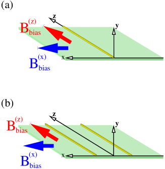
Figure 1: Setup of the atom chip showing directions of the wires and the magnetic bias fields needed to form the trapping potential. (a) Single-wire trap. (b) Double-wire trap.

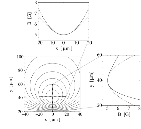
Figure 2: Contour-plot of the magnetic field of the single-wire trap for $B^{(x)}_{\mathrm{bias}}=10{\mathrm{G}}$, $B^{(z)}_{\mathrm{bias}}=5{\mathrm{G}}$, and $I=0.1{\mathrm{A}}$. The upper (right) plot shows a horizontal (vertical) cut through the potential minimum. The dashed lines in the upper and the right plot show the harmonic approximation to the trapping field.

II.1 Stochastic equation for the density matrix

The quantum mechanical evolution of a cold atomic cloud is described by a density matrix. The time evolution of the density matrix $\rho({\bf x},{\bf x}^{\prime},t)$ is given by the von Neumann equation

$$i\hbar\frac{\partial}{\partial t}\rho=[H,\rho]\;,$$ (2)

where $H$ is the Hamiltonian of an atom in the trapping potential:

$$H=\frac{{\bf p}^{2}}{2m}+V_{t}({\bf r}_{\perp})+\delta V({\bf x},t)\;.$$ (3)

Here, $V_{t}({\bf r}_{\perp})$ is the confining potential which we will assume to be constant along the trap, and $\bf r_{\perp}$ denotes the coordinate perpendicular to the direction of the current-carrying wire or the wave guide. The last term $\delta V({\bf x},t)$ is a random fluctuation term induced by the current noise.

We will formulate the problem for a system of $N$ parallel quasi-1d magnetic traps generated by a set of $M$ parallel wires on the chip (in general, $N\neq M$ since some of the magnetic-field minima may merge). The number of parallel trapping wells is included in the structure of the confining potential $V_{t}({\bf r}_{\perp})$. In all further calculations we will assume that the surface of the atom chip is in the $\hat{x}$-$\hat{z}$ plane and that the atoms are trapped in the half space $y>0$ above the chip. The wires on the atom chip needed to form the trapping field, are assumed to be aligned in $\hat{z}$-direction.

In position representation for the density matrix the von Neumann equation reads

$$i\hbar\frac{\partial}{\partial t} \rho({\bf x},{\bf x}^{\prime},t)=\Big{[}-\frac{\hbar^{2}}{2m}\left(\frac{d^{2}}{d{\bf x}^{2}}-\frac{d^{2}}{d{\bf x}^{\prime^{2}}}\right)+V_{t}({\bf r}_{\perp})$$

$$-V_{t}({\bf r}_{\perp}^{\prime})+\delta V({\bf x},t)-\delta V({\bf x}^{\prime},t)\Big{]}\rho({\bf x},{\bf x}^{\prime},t)\;.$$

To derive a quasi-1d expression for Eq. (II.1) we expand the density matrix in eigenmodes of the transverse potential $\chi_{n}({\bf r}_{\perp})$:

$$\rho({\bf x},{\bf x}^{\prime},t)=\sum_{n,m}\chi_{n}^{*}({\bf r}_{\perp})\chi_{m}({\bf r}_{\perp}^{\prime})\rho_{nm}(z,z^{\prime},t)\;.$$ (5)

Here, the channel index $n$ labels the transverse states of the trapping potential. The transverse wavefunctions $\chi_{n}({\bf r}_{\perp})$ are chosen mutually orthogonal and are eigenfunctions of the transverse part of the Hamiltonian in Eq. (3) in the sense that

$$\left[-\frac{\hbar^{2}}{2m}\nabla^{2}_{{\bf r}_{\perp}}+V_{t}({\bf r}_{\perp})\right]\chi_{n}({\bf r}_{\perp})=E_{n}\chi_{n}({\bf r}_{\perp})\;.$$ (6)

The decomposition (5) in transverse and longitudinal components of the density matrix is now inserted in the von Neumann equation, Eq. (II.1). Making use of the orthogonality and the completeness of the transverse states $\chi_{n}({\bf r}_{\perp})$ we obtain a one-dimensional equation for the evolution of the density matrix:

$$\left[i\hbar\frac{\partial}{\partial t}+\frac{\hbar^{2}}{2m}\left(\frac{d^{2}}{dz^{2}}-\frac{d^{2}}{dz^{\prime^{2}}}\right)-\Delta E_{lk}\right]\rho_{lk}(z,z^{\prime},t)$$ (7)

$$=\sum_{n}\left[\delta S_{ln}(z,t)\rho_{nk}(z,z^{\prime},t)-\delta S_{nk}(z^{\prime},t)\rho_{ln}(z,z^{\prime},t)\right]\;.$$

Here the abbreviation $\Delta E_{lk}=E_{l}-E_{k}$ was introduced for the difference of transverse energy levels, and the fluctuations $\delta S_{nk}(z)$ are defined as

$$\delta S_{nk}(z,t)=\int d{\bf r}_{\perp}\;\chi_{n}({\bf r}_{\perp})\delta V({\bf x},t)\chi_{k}^{*}({\bf r}_{\perp})\;.$$ (8)

The left-hand side of the reduced von Neumann equation, Eq. (7), describes the evolution of an atom wavefunction in the non-fluctuating trapping potential and we will hereafter abbreviate this part by $(i\hbar\partial_{t}-\hat{H}_{lk})$. The terms on the right-hand side of Eq. (7) contain the influence of the potential fluctuations.

The fluctuations of the confining potential are described by the matrix elements $\delta S_{nk}(z,t)$ which imply transitions between different discrete transverse energy levels induced by the fluctuating potential. The influence of the fluctuating potential onto the longitudinal motion of the atomic cloud is included in the $z$ dependence of $\delta S_{nk}(z,t)$.

II.2 Averaged equation of motion for the density matrix

In this section we derive the equation of motion describing the evolution of the density matrix $\langle\rho\rangle$ averaged over the potential fluctuations Gardiner01 ; vanKampen . To keep the expressions compact we rewrite Eq. (7) as

$$\left(i\hbar\partial_{t}-\tilde{H}\right)\rho=\delta\tilde{S}\rho\;,$$ (9)

where the spatial coordinates ${\bf x}$, ${\bf x}^{\prime}$, time $t$ and all indices have been suppressed. The components of the quantities $\tilde{H}$ and $\delta\tilde{S}$ are defined as

$$\tilde{H}_{lkij} = \hat{H}_{lk}\delta_{li}\delta_{kj}\,,$$ (10)

$$\delta\tilde{S}_{lkij} = \delta S_{li}(z,t)\delta_{kj}-\delta S_{jk}(z^{\prime},t)\delta_{li}\,.$$ (11)

The product in (9) has the meaning $\tilde{A}\rho=\sum_{ij}A_{lkij}\rho_{ij}$. The stochastic equation (9) for the density matrix is averaged over the fluctuating potential using the standard cumulant expansion vanKampen . Writing the time arguments again we obtain

$$\left(i\hbar\partial_{t}-\tilde{H}\right)\langle\rho(t)\rangle=\langle\delta\tilde{S}(t)\rangle\langle\rho(t)\rangle-\frac{i}{\hbar}\int^{t}_{0}dt^{\prime}\langle\langle\delta\tilde{S}(t)e^{-\frac{i}{\hbar}\tilde{H}t^{\prime}}\delta\tilde{S}(t-t^{\prime})\rangle\rangle e^{\frac{i}{\hbar}\tilde{H}t^{\prime}}\langle\rho(t)\rangle\;.$$ (12)

Here, the brackets $\langle\,\cdot\,\rangle$ denote the averaging over all realisations of the potential fluctuations and the double brackets $\langle\langle\,\cdot\,\rangle\rangle$ denote the second cumulant. We can take the mean value of the potential fluctuation $\langle\delta V\rangle$ to zero, since the static potential is already included in the Hamiltonian on the left hand side of Eq. (12) and, hence, the first term on the right-hand side of Eq. (12) vanishes.

Reinserting the explicit expressions for $\tilde{H}$, $\delta\tilde{S}$ leads to the desired equation of motion for the density matrix

$$\left(i\hbar\partial_{t}-\hat{H}_{lk}\right)\langle\rho_{lk}(z,z^{\prime},t)\rangle=-\frac{i}{\hbar}\sum_{ijmn}\int\limits^{t}_{0}d\tau\int\limits^{\infty}_{-\infty}d\tilde{z}\int\limits^{\infty}_{-\infty}d\tilde{z}^{\prime}K_{ij}(z-\tilde{z},z^{\prime}-\tilde{z}^{\prime},t-\tau)$$ (13)

$$\times\left[\langle\delta S_{li}(z,t)\delta S_{im}(\tilde{z},\tau)\rangle\delta_{kj}\delta_{jn}+\langle\delta S_{jk}(z^{\prime},t)\delta S_{nj}(\tilde{z}^{\prime},\tau)\rangle\delta_{li}\delta_{im}\right.$$

$$\left.-\langle\delta S_{li}(z,t)\delta S_{nj}(\tilde{z}^{\prime},\tau)\rangle\delta_{im}\delta_{jk}-\langle\delta S_{jk}(z^{\prime},t)\delta S_{im}(\tilde{z},\tau)\rangle\delta_{jn}\delta_{li}\right]\langle\rho_{mn}(\tilde{z},\tilde{z}^{\prime},\tau)\rangle\,.$$

The kernel $K_{ij}(z-\tilde{z},z^{\prime}-\tilde{z}^{\prime},t)$ is the Fourier transform of

$$K_{ij}(q,q^{\prime},t)=\exp\left(-i\frac{\hbar}{2m}\left(q^{2}-{q^{\prime}}^{2}\right)t-\frac{i}{\hbar}\Delta E_{ij}t\right)\;,$$ (14)

which can be explicitly evaluated, but this has no advantage for our further discussion.

Equation (13) is the main result of this section. It describes the evolution of the density matrix in a quasi-1d waveguide under the influence of an external noise source. It is valid for an arbitrary form of the transverse confining potential, thus, in particular, for single and double-wire traps. The main input is the external noise correlator and its effect on the trapped atoms. The noise correlator depends on the concrete wire configuration. Below we will derive a simplified form of the equation of motion (13) under the assumption that the time scale characterizing the fluctuations is much shorter than the time scales of the atomic motion.

II.3 Noise correlation function

We will now derive the noise correlator for our specific system and use Eq. (13) to study the dynamics. As we are interested in the coherence of atoms in an atom-chip trap, we will consider the current noise in the wires as the decoherence source. Fluctuations of the magnetic bias fields $B^{(x)}_{\textrm{bias}}$ and $B^{(z)}_{\textrm{bias}}$, needed to form the trapping potential, will be neglected.

Using the approximation of a 1d wire, the fluctuating current density can be written as

$${\bf j}({\bf x},t)=I(z,t)\delta(x)\delta(y)\hat{{\bf z}}\;,$$ (15)

where $\hat{\bf z}$ is the unit vector in $\hat{z}$-direction. The fluctuations of the current density are defined by $\delta{\bf j}({\bf x},t)\equiv{\bf j}({\bf x},t)-\langle{\bf j}({\bf x})\rangle$. It is sufficient to know $\langle\delta I(z,t)\delta I(z^{\prime},t^{\prime})\rangle$ to obtain the full current density correlation function $\langle\delta{\bf j}({\bf x})\delta{\bf j}({\bf x}^{\prime})\rangle$. Note, that the average currents are already included in the static potential $V_{t}(\bf r_{\perp})$.

The restriction of ${\bf j}$ to the ${\bf\hat{z}}$ direction is a reasonable assumption since we consider micro-structured wires with small cross-section $A=l_{w}l_{h}$, i.e. wires with widths $l_{w}$ and heights $l_{h}$ much smaller than the trap-to-wire distance $r_{0}$. Transversal current fluctuations lead to surface charging and thus to an electrical field which points in opposite direction to the current fluctuation. This surface charging effect will suppress fluctuations which are slow compared to $\omega_{RC}=\sigma\Lambda/\epsilon_{0}\l_{w}$. Here, $\sigma$ is the conductivity of the wire, $\epsilon_{0}$ the (vacuum) dielectric constant, and $\Lambda\approx 1\mbox{\AA}$ is the screening length in the metal. This leads to RC-frequencies of $\omega_{RC}\approx 10^{13}{\mbox{Hz}}$ for wire widths of $l_{w}=10\mu\mbox{m}$ and typical values for the conductivity in a metal.

The characteristic time scale for the atomic motion in the trap is given by the frequency of the trapping potential $\omega\approx 10^{4}\mbox{Hz}$. Thus, considering atomic traps with $\omega\ll\omega_{RC}$ the current fluctuations can be taken along ${\bf\hat{z}}$ as a direct consequence of the quasi-one-dimensionality of the wire.

The current fluctuations are spatially uncorrelated as they have their origin in electron scattering processes. Hence, the correlator $\langle\delta I(z)\delta I(z^{\prime})\rangle$ has the form deJong01 ; Blanter01

$$\langle\delta I(z,t)\delta I(z^{\prime},t^{\prime})\rangle=4k_{\textrm{B}}T_{\textrm{eff}}(z)\sigma A\,\delta(z-z^{\prime})\delta_{c}(t-t^{\prime})\;.$$ (16)

Here, $k_{\textrm{B}}$ is the Boltzmann constant. The effective noise temperature is given by deJong01 ; Blanter01

$$T_{\textrm{eff}}(z)=\int dEf(E,z)[1-f(E,z)]\;,$$ (17)

where $f(E,z)$ is the energy- and space-dependent non-equilibrium distribution function. A finite voltage across the wire induces a change in the velocity distribution of the electrons and the electrons are thus no longer in thermal equilibrium. Nevertheless, the deviation from an equilibrium distribution is small at room temperature due to the large number of inelastic scattering processes. The effective temperature $T_{\mathrm{eff}}$ accounts for possible non-equilibrium effects such as shot noise. However, contributions of non-equilibrium effects to the noise strongly depend on the length $L$ of the wire compared to the characteristic inelastic scattering lengths. E.g. strong electron-phonon scattering leads to an energy exchange between the lattice and the electrons. The non-equilibrium distribution is ’cooled’ to an equilibrium distribution at the phonon temperature. Thus, non-equilibrium noise sources, such as shot noise, are strongly suppressed for wires much longer than the electron-phonon scattering length $l_{\mathrm{ep}}$ and the noise in the wire is essentially given by the equilibrium Nyquist noise deJong01 ; Nagaev01 ; Kozub01 . As the wire lengths used in present experiments are much longer than $l_{\mathrm{ep}}$, we $T_{\mathrm{eff}}\approx 300{\mathrm{K}}$ in all our calculations.

Finally,

$$\delta_{c}(t)=\frac{1}{\pi}\frac{\tau_{c}}{t^{2}+\tau^{2}_{c}}$$ (18)

is a representation of the delta function. The correlation time $\tau_{c}$ is given by the time scale of the electronic scattering processes.

II.4 Simplified equation of motion

The dominating source of the current noise in the wires is due to the scattering of electrons with phonons, electrons and impurities. These scattering events are correlated on a time scale much shorter than the characteristic time scales of the atomic system. This separation of time scales allows us to simplify the equation of motion (13).

As a consequence of Eq. (16), the correlation function of the fluctuating potential will be of the form

$$\langle\delta V({\bf x},t)\delta V({\bf x}^{\prime},t^{\prime})\rangle=\delta_{c}(t-t^{\prime})\langle\delta V({\bf x})\delta V({\bf x}^{\prime})\rangle\;.$$ (19)

Using Eq. (8) we obtain

$$\langle\delta S_{im}(z,t)\delta S_{nj}(z^{\prime},t^{\prime})\rangle=\delta_{c}(t-t^{\prime})\langle\delta S_{im}(z)\delta S_{nj}(z^{\prime})\rangle$$ (20)

for the fluctuations of the projected potential.

We replace all the correlation functions in the equation of motion (13) by the expression (20). The time integration can be performed using the fact that the averaged density matrix $\langle\rho(\tau)\rangle$ varies slowly on the correlation time scale $\tau_{c}$. Thus, $\langle\rho(\tau)\rangle$ can be evaluated at time $t$ and taken out of the time integral. Finally, taking $\tau_{c}$ to zero, the Fourier transform of the kernel (14) leads to a product of delta functions in the spatial coordinates. Performing the remaining spatial integrations over $\tilde{z}$ and $\tilde{z}^{\prime}$, Eq. (13) reduces to

$$\left(i\hbar\partial_{t}-\hat{H}_{lk}\right)\langle\rho_{lk}(z,z^{\prime},t)\rangle=-\frac{i}{2\hbar}\sum_{mn}\left[\langle\delta S_{ln}(z)\delta S_{nm}(z)\rangle\langle\rho_{mk}(z,z^{\prime},t)\rangle\right.$$ (21)

$$+\langle\delta S_{mk}(z^{\prime})\delta S_{nm}(z^{\prime})\rangle\langle\rho_{ln}(z,z^{\prime},t)\rangle\left.-2\langle\delta S_{lm}(z)\delta S_{nk}(z^{\prime})\rangle\langle\rho_{mn}(z,z^{\prime},t)\rangle\right]\,.$$

The trapping potential has $N$ minima, i.e., the channel index $n$ can be written as $n=(\alpha,n_{x},n_{y})$, $\alpha=1,...,N$. We will now assume that the minima are well-separated in $\hat{x}\hat{y}$-direction such that we can neglect all matrix elements $\delta S_{ij}$ with different trap labels $\alpha$. Under this assumption, the first and second term on the right-hand side of Eq. (21) depend only on a single trap label. In the third term, the trap labels may be different for $\delta S_{lm}$ as compared to $\delta S_{nk}$. Since current noise in one particular wire generates fluctuations of the magnetic field in all trapping wells, there will be a correlation between the fluctuations in different traps. It is hence this third term in Eq. (21) which describes the correlation between potential fluctuations in different traps.

Using Eq. (21) it is now possible to describe decoherence induced by current noise in trapping geometries of one, two or more parallel wires Reichel02 ; Folman01 . In the following sections we will discuss decoherence in two specific trapping configurations: the single-wire trap in Section III.1, and the double-wire trap in Section III.2, which is of particular interest for atom interferometry experiments Hinds01 ; Andersson01 ; Haensel03 .

III Trapping Geometries

We will now consider two specific trap configurations, the single-wire trap and the double-wire trap. The dynamics of the noise-averaged density matrix will be discussed using Eq. (21) which was derived in the previous section. We assume that the wire generating the potential fluctuations is one-dimensional. This assumption is reasonable for distances $r_{0}$ of the trap minimum to the wire much larger than the wire width $l_{w}$ and wire height $l_{h}$. Typical length scales are $r_{0}\approx~{}10\mu$m to $1$mm and wire widths and heights $l_{w}\approx 10\mu$m to $50\mu$m, $l_{h}\approx 1\mu$m Folman01 .

To keep the notation short, we will suppress the brackets denoting the averaging. Thus, from now on, the density matrix $\rho_{ij}$ denotes the average density matrix.

III.1 The single-wire trap

We are now looking at a specific magnetic trapping field having only a single one-dimensional trapping well as shown in Fig. 2. The magnetic field is generated by the superposition of the magnetic field due to the current $I$ in the single wire along the $\hat{z}$-axis and a homogeneous bias field $B^{(x)}_{\textrm{bias}}$ parallel to the chip surface and perpendicular to the wire (see Fig. 1). We additionally include a homogeneous bias field $B^{(z)}_{\textrm{bias}}$ parallel to the trapping well. This longitudinal bias field is experimentally needed to avoid spin flips at the trap center. Thus the magnetic field has the form:

$${\bf B}({\bf x})=\frac{\mu_{0}I}{2\pi}\frac{1}{x^{2}+y^{2}}\left(\begin{array}[]{c}-y\\ x\\ 0\end{array}\right)+\left(\begin{array}[]{c}B^{(x)}_{\textrm{bias}}\\ 0\\ B^{(z)}_{\textrm{bias}}\end{array}\right).$$ (22)

The minimum of the trapping potential is located above the wire $x_{0}=0$ and has a wire-to-trap distance of $r_{0}=y_{0}=\mu_{0}I/(2\pi B^{(x)}_{\textrm{bias}})$.

We have now all the ingredients needed to calculate the fluctuation-correlator $\langle\delta S_{im}(z)\delta S_{nj}(z^{\prime})\rangle$. Using Eqs. (8), (15), and (16) we obtain

$$\langle\delta S_{im}(z)\delta S_{nj}(z^{\prime})\rangle=A_{imnj}J(z-z^{\prime})\;.$$ (23)

The transition matrix elements are given by

$$\begin{split}A_{imnj}=&\quad k_{\textrm{B}}T_{\textrm{eff}}\sigma A\left(\frac{\mu_{0}g_{F}\mu_{B}}{\pi}\frac{B^{(x)}_{\textrm{bias}}}{B^{(z)}_{\textrm{bias}}}\right)^{2}\\ &\times\int d{\bf r}_{\perp}\;\chi_{i}({\bf r}_{\perp})(y-y_{0})\chi_{m}^{*}({\bf r}_{\perp})\\ &\times\int d{\bf r}^{\prime}_{\perp}\;\chi_{n}({\bf r}^{\prime}_{\perp})(y^{\prime}-y_{0})\chi_{j}^{*}({\bf r}^{\prime}_{\perp})\;.\end{split}$$ (24)

The spatial dependence of the noise correlator is given by

$$J(z)=\frac{1}{r^{5}_{0}}\int\limits^{\infty}_{-\infty}d\tilde{z}\left[1+\tilde{z}^{2}\right]^{-\frac{3}{2}}\left[1+\left(z/r_{0}-\tilde{z}\right)^{2}\right]^{-\frac{3}{2}}\;.$$ (25)

A more detailed derivation of the correlation function is given in Appendix A. The integration in Eq. (24) can be done explicitly using harmonic oscillator states for $\chi_{n}({\bf r}_{\perp})$, which is a good approximation as long as $B^{(z)}_{\textrm{bias}}$ is of the order of $B^{(x)}_{\textrm{bias}}$ and the wire-to-trap distance $r_{0}$ is much larger than the transverse width $w$ of the trapped state. Both requirements are usually well satisfied in experiments. The dashed line in Fig. 2 shows the harmonic approximation to the trapping potential. Using the harmonic approximation we can characterize the steepness of the trapping potential by its trap frequencies. It turns out that the two frequencies coincide,

$$\omega=\sqrt{\frac{2\mu_{B}g_{F}}{mB^{(z)}_{\textrm{bias}}}}\frac{B^{(x)}_{\textrm{bias}}}{y_{0}}\;,$$ (26)

i.e., the trap potential can be approximated by an isotropic 2d harmonic oscillator (2d-HO).

After integration we obtain

$$A_{imnj}=A_{0}\;\delta_{i_{x}m_{x}}\tilde{\delta}_{i_{y}m_{y}}\delta_{n_{x}j_{x}}\tilde{\delta}_{n_{y}j_{y}}\;,$$ (27)

where

$$\tilde{\delta}_{i_{y}m_{y}}=\sqrt{m_{y}+1}\;\delta_{i_{y},m_{y}+1}+\sqrt{m_{y}}\;\delta_{i_{y},m_{y}-1}\;,$$ (28)

and the indices $n_{x}$, $n_{y}$ denote the energy levels in $\hat{x}$ and $\hat{y}$ direction of the 2d-HO. The prefactor $A_{0}$ is

$$A_{0}=k_{\textrm{B}}T_{\textrm{eff}}\sigma A\left(\frac{\mu_{0}g_{F}\mu_{B}}{\pi}\frac{B^{(x)}_{\textrm{bias}}}{B^{(z)}_{\textrm{bias}}}\right)^{2}\frac{w^{2}}{2}$$ (29)

and $w=\sqrt{\hbar/(m\omega)}$ is the oscillator length of the harmonic potential.

Before moving on to derive the equation of motion for the averaged density matrix, let us discuss some consequences of expression (27). Inspection of the coefficients $A_{imnj}$ in Eq. (27) shows that there is no direct influence onto the longitudinal motion of the atom, since the matrix element $A_{iijj}$ vanishes. This result is not unexpected, because we consider only current fluctuations along the wire, which give rise to fluctuations in the trapping field along the transverse directions of the trap potential. In fact, only transitions among energy levels of the $\hat{y}$-component of the 2d-HO give a non-vanishing contribution. An explanation can be obtained by examining the change of the trap minimum position under variation of the current in the wire. Changing the current by $\delta I$ leaves the trap minimum in $\hat{x}$-direction unchanged at $x_{0}=0$, but shifts the $\hat{y}$-trap minimum by $\delta y_{0}=\mu_{0}\delta I/(2\pi B^{(x)}_{\textrm{bias}})$ misalign . Even though there is no direct coupling to the motion along the wire there can still be spatial decoherence in $\hat{z}$-direction as we will see in the final result for $\rho$ obtained from Eq. (21). However, this requires transitions to neighbouring transverse energy levels.

Substituting Eqs. (23) and (27) in Eq. (21) leads to an equation of motion for $\rho$ for the single-wire trap configuration. Instead of discussing the general equation of motion of $\rho$ we will only consider the case where the two lowest energy levels of the transverse motion are taken into account. The restriction to the lowest energy levels corresponds to the situation of the atomic cloud being mostly in the ground state of the trap and having negligible population of higher energy levels. This situation is realistic, if the energy spacing of the discrete transverse states is large compared to the kinetic energy. Nevertheless, the result obtained from the two-level model provides a reasonable estimate for the decoherence of an atomic cloud, even if many transverse levels are populated. Equation (27) shows that only next-neighbour transitions are allowed. As $A_{imnj}$ is a product of two next-neighbour transitions there can only be contributions of the next two neighbouring energy levels. Higher energy levels do only contribute to the decoherence by successive transitions which are of higher order in $A_{imnj}$ and hence are negligible.

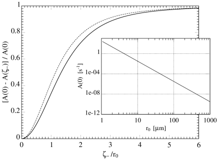
Figure 3: Spatial dependence of the decay rate $\bar{\Gamma}_{\mathrm{dec}}(\zeta_{-})=A(0)-A(\zeta_{-})$ for the diagonal elements $\bar{\rho}_{ii}(\zeta_{-},t)$, Eq. (37). The wire-to-trap distance is $r_{0}=100\mu\textrm{m}$ and the trap frequency is $\omega\approx 2\pi\times 10\textrm{kHz}$. The dashed line is the approximation Eq. (39) for $A(\zeta_{-})$. Inset: Decay rate $A(0)$ as function of $r_{0}$. The parameters chosen in the plots correspond to ${}^{87}\textrm{Rb}$ trapped at $T_{\textrm{eff}}=300\textrm{K}$ in a magnetic trap with a gold wire of conductivity $\sigma_{\textrm{Au}}~{}=~{}4.54\cdot 10^{7}\Omega^{-1}\textrm{m}^{-1}$ and a cross-section of $A=2.5\mu{\textrm{m}}\times 5\mu{\textrm{m}}$. The bias fields chosen are $B^{(x)}_{\textrm{bias}}=80\textrm{G}$ and $B^{(z)}_{\textrm{bias}}=2\textrm{G}$.

We rewrite Eq. (21) for the subspace of the two lowest eigenstates in a matrix equation for the density vector

$${\bf{\rho}}=\left(\rho_{00},\rho_{11},\rho_{10},\rho_{01}\right)\;.$$ (30)

The indices of the averaged density matrix $\rho_{lk}$ denote the transverse state $l=(l_{x},l_{y})$ but we are only writing the $l_{y}$ component of the label as $\rho$ can only couple to states with the same $x$-state (i.e. only transitions between different $y$-states of the 2d-HO are allowed). The $x$-label is $l_{x}=0$ for all states under consideration. Hence Eq. (21) can be written as a matrix equation for the density matrix vector Eq. (30)

$$\left[i\hbar\partial_{t}-\tilde{H}(z,z^{\prime})\right]{\bf{\rho}}(z,z^{\prime},t)=-i\hbar\tilde{A}(z-z^{\prime}){\bf{\rho}}(z,z^{\prime},t)\,.$$ (31)

The matrix $\tilde{A}$ is defined as

$$\tilde{A}(\zeta_{-})=\left(\begin{array}[]{cccc}A(0)&-A(\zeta_{-})&0&0\\ -A(\zeta_{-})&A(0)&0&0\\ 0&0&A(0)&-A(\zeta_{-})\\ 0&0&-A(\zeta_{-})&A(0)\end{array}\right)\,,$$ (32)

where $A(\zeta_{-})=\frac{1}{\hbar^{2}}A_{0}J(\zeta_{-})$ and $\zeta_{-}=z-z^{\prime}$. The equations for the diagonal elements, i.e., $\rho_{00}$, $\rho_{11}$, and for the off-diagonal elements, i.e. $\rho_{01}$, $\rho_{10}$ decouple. However, the decoupling is a consequence of the restriction to the two lowest energy levels and is not found in the general case. Yet, the decoupling allows to find an explicit solution for the time evolution of the diagonal elements. The matrix equation proves to be diagonal for the linear combinations $\rho^{\pm}\equiv\rho_{00}\pm\rho_{11}$ and introducing the new coordinates $\zeta_{-}=z-z^{\prime}$ , $\zeta_{+}=\frac{1}{2}(z+z^{\prime})$ we obtain the general solution

$$\rho^{\pm}_{k}(\zeta_{-},\zeta_{+},t)=R^{\pm}_{k}(\zeta_{-}-\frac{\hbar k}{m}t)e^{ik\zeta_{+}}e^{-\Gamma^{\pm}_{k}(\zeta_{-},t)t}\;,$$ (33)

where the decay is described by

$$\Gamma^{\pm}_{k}(\zeta_{-},t)=A(0)\mp\frac{1}{t}\int\limits_{0}^{t}dt^{\prime}A(\zeta_{-}-\frac{\hbar k}{m}t^{\prime})\,.$$ (34)

The function $R^{\pm}_{k}$ is fixed by the initial conditions, i.e. by the density matrix at time $t=0$ :

$$R^{\pm}_{k}(\zeta_{-})=\int\limits_{-\infty}^{\infty}d\zeta_{+}e^{-ik\zeta_{+}}\rho^{\pm}(\zeta_{-},\zeta_{+},t=0)\,.$$ (35)

Note that $\Gamma$ in Eq. (34) is a function of the spatial variable $\zeta_{-}$ and the wavevector $k$, and is in general not linear in the time argument $t$. Adding and subtracting the contributions $\rho^{\pm}$ finally leads to the following expressions for the diagonal elements of the density matrix

$$\rho_{00}(\zeta_{-},\zeta_{+},t)=\frac{1}{2}\int\limits_{-\infty}^{\infty}\frac{dk}{2\pi}[\rho^{+}_{k}(\zeta_{-},\zeta_{+},t)+\rho^{-}_{k}(\zeta_{-},\zeta_{+},t)]\,.$$ (36)

The result for $\rho_{11}$ can be obtained from (36) by replacing the plus sign between the terms by a minus sign. To get a feeling for the spatial correlations we trace out the center of mass coordinate $\zeta_{+}$ :

$$\bar{\rho}_{00}(\zeta_{-},t) = \int_{-\infty}^{\infty}d\zeta_{+}\;\rho_{00}(\zeta_{-},\zeta_{+},t)$$ (37)

$$= e^{-\left[A(0)-A(\zeta_{-})\right]t}$$

$$\times \frac{1}{2}\left[\bar{\rho}_{00}(\zeta_{-},0)\left(1+e^{-2A(\zeta_{-})t}\right)\right.$$

$$+ \left.\bar{\rho}_{11}(\zeta_{-},0)\left(1-e^{-2A(\zeta_{-})t}\right)\right]\;.$$

Equation (37) shows that we can distinguish two decay mechanisms. There is an overall decay of the spatial off-diagonal elements with a rate $\bar{\Gamma}_{\textrm{dec}}(\zeta_{-})=[A(0)-A(\zeta_{-})]$. This decay only affects the density matrix for $\zeta_{-}\neq 0$, thus suppressing the spatial coherence. The spatial correlation of the potential fluctuations can be read off Fig. 3, showing $\bar{\Gamma}_{\textrm{dec}}(\zeta_{-})$. We find for the potential fluctuations a correlation length $\xi_{c}$ of the order of the trap-to-chip surface distance $\xi_{c}\approx r_{0}$. The correlation length $\xi_{c}$ must not be confused with the coherence length describing the distance over which the transport of an atom along the trapping well is coherent. This coherence length is described by the decoherence time and the speed of the moving wavepacket. The correlation length $\xi_{c}$ characterizes the distance over which the potential fluctuations are correlated.

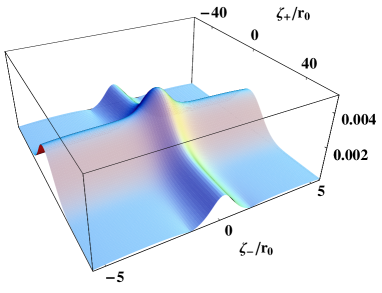
Figure 4: Time evolution of $|\rho_{00}(\zeta_{-},\zeta_{+},t)|$ after $t=2/A(0)$. At $t=0$ the wavepacket is a Gaussian wavepacket of spatial extent $w_{z}=20r_{0}$. The wire-to-trap distance is $r_{0}=5\mu\textrm{m}$ and all other parameters correspond to those used in Fig. 3. $A(0)\approx 0.5{\mathrm{s}}^{-1}$ is given by Eq. (38). The density matrix shows damped oscillations which become more pronounced as $\zeta_{+}$ increases.

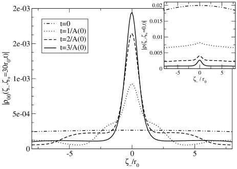
Figure 5: Decay of the absolute value $|\rho_{00}(\zeta_{-},\zeta_{+}=30r_{0},t)|$ and $|\rho_{00}(\zeta_{-},\zeta_{+}=0,t)|$ (inset). The wave packet is a Gaussian wavepacket of spatial extent $w_{z}=20r_{0}$ at $t=0$. The wire-to-trap distance is $r_{0}=5\mu\textrm{m}$. All other parameters are the same as used in Fig. 3. $A(0)\approx 0.5{\mathrm{s}}^{-1}$ is given by Eq. (38). The dashed line ($t=2/A(0)$) corresponds to cuts of Fig. 4 along $\zeta_{-}$ for $\zeta+=30r_{0}$ (inset $\zeta_{+}=0$). Spatial correlations of the potential fluctuations are restricted to a narrow band around $\zeta_{-}=0$. The width of this band is on the order of $r_{0}$. The density matrix shows damped oscillations which become more pronounced with increasing $\zeta_{+}$. The increase of $|\rho_{00}(\zeta_{-},\zeta_{+}=30r_{0},t)|$ for increasing time $t$ is a consequence of the spreading of the wavepacket.

The second mechanism describes the equilibration of excited and ground state, quantified by the diagonal elements $\bar{\rho}_{00}(0,t)$, which occurs at a rate $\bar{\Gamma}_{\textrm{pop}}(0)=2A(0)$. Here equilibration means that, due to this mechanism, the probability to be in the ground state, i.e. $\rho_{00}(0,t)$, tends to 1/2. Of course, at the same time the probability $\rho_{11}(0,t)$ to be in the excited state approaches 1/2 at the same rate. Note, that for the spatial off-diagonal matrix elements the equilibration rate depends on $\zeta_{-}$.

We will now take a closer look onto the quantity $A(0)$ for realistic trap parameters. Using $J(0)=\frac{3\pi}{8y_{0}^{5}}$ and Eq. (26), Eq. (29) leads to

$$A(0)=\frac{3\pi}{2}k_{\textrm{B}}T_{\textrm{eff}}\sigma A\frac{B^{(x)}_{\textrm{bias}}}{2\hbar\sqrt{m}}\left(\frac{\mu_{0}}{4\pi}\right)^{2}\left(\frac{2\mu_{B}g_{F}}{B^{(z)}_{\textrm{bias}}}\right)^{\frac{3}{2}}\frac{1}{r_{0}^{4}}\;.$$ (38)

The inset of Fig. 3 plots $A(0)$ over $r_{0}$ for reasonable trap parameters. Equation (38) shows that the decay rate is scaling on the wire-to-trap distance as $1/r_{0}^{4}$ giving a rapid increase of decoherence effects once the atomic cloud is brought close to the wire.

As specific example we want to study the time evolution of the full density matrix in the ground state. Figure 4 and Fig. 5 show the time evolution of the absolute value of the density matrix element $|\rho_{00}(\zeta_{-},\zeta_{+},t)|$ for a Gaussian wave packet of spatial extent $w_{z}=20r_{0}$ and a wire-to-trap distance of $r_{0}=5\mu\textrm{m}$. Initially, at time $t=0$ all other elements of the density matrix are zero. The time evolution is calculated for the reduced subspace using Eq. (33) and Eq. (36). For the spatial correlation we use the approximation (dashed line in Fig. 3)

$$A(\zeta_{-})\approx 4\frac{A_{0}}{\hbar^{2}r_{0}^{5}}\left[\left(\frac{32}{3\pi}\right)^{\frac{2}{3}}+\left(\frac{\zeta_{-}}{r_{0}}\right)^{2}\right]^{-\frac{3}{2}}\,.$$ (39)

The time evolution of the Gaussian wavepacket shows a strip of $|\zeta_{-}|<l_{c}\approx r_{0}$ in which the density matrix decays much slower. This is a consequence of the $\zeta_{-}$ dependence of the decay rate shown in Fig. 3. The spatial correlation length of the wavepacket can hence be read of Fig. (5) as $l_{c}\approx r_{0}$. In addition, a damped oscillation in the relative coordinate $\zeta_{-}$ is arising which is getting more pronounced for larger values of $\zeta_{+}$. Figure 5 shows cuts along the $\zeta_{-}$-direction for different values of $\zeta_{+}$. The origin of the damped oscillations is the $k$-dependence of the equilibration and decoherence mechanism described by $\Gamma^{\pm}_{k}$ in Eq. (34). To demonstrate the influence of the $k$-dependent damping we assume that $\Gamma^{\pm}_{k}=A(0)\mp[A(\zeta_{-})+\beta(\zeta_{-},t)k]$. Choosing $\Gamma$ linear in $k$ leads to a modulation of the density matrix by a factor proportional to $\cosh(i\alpha_{0}\beta+\alpha_{1})$, describing damped oscillations. The $\alpha_{0/1}$ are real functions of $\zeta_{\pm}$ and $t$. The oscillations arise only for non-vanishing $\beta$. Decay rates which are $k$-independent do not show oscillations.

The decay described by $\Gamma^{\pm}_{k}$ in Eq. (34) is however not linear, but includes higher powers in $k$. Hence the simple linear model $\Gamma^{\pm}_{k}=A(0)\mp[A(\zeta_{-})+\beta(\zeta_{-},t)k]$ describes the oscillations in Fig. 4 and Fig. 5 only qualitatively.

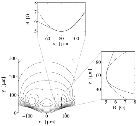
Figure 6: Contour-plot of the magnetic field in the double-wire geometry for $B^{(x)}_{\mathrm{bias}}=10{\mathrm{G}}$, $B^{(z)}_{\mathrm{bias}}=5{\mathrm{G}}$, and $I=0.3{\mathrm{A}}$. The wires are located at $x=\pm 100\mu$m and $y=0$. Two potential minima are located roughly above the current-carrying wires. The upper (right) plot shows a horizontal (vertical) cut through the right potential minimum. The dashed lines in the upper and the right plot show the harmonic approximation to the trapping field.

III.2 The double-wire trap

The second configuration which we discuss is a double-wire trap Hinds01 . A system of two parallel trapping wells is of special interest for high-precision interferometry Hinds01 ; Andersson01 ; Haensel03 or beam-splitter geometries Andersson02 . The effect of decoherence is one of the key issues in these experiments.

Form and characteristic of the double-wire trap is described in Hinds01 ; Folman01 so that we will only briefly introduce the main features of the double-wire trapping potential. Figure 1b shows the setup for the trapping field, which is generated by two infinite wires running parallel to the $\hat{z}$-axis, separated by a distance $d$, and a superposed homogeneous bias field $B^{(x)}_{\textrm{bias}}$ perpendicular to the current direction. A second bias field pointing along the $\hat{z}$-direction, $B^{(z)}_{\textrm{bias}}$, is added in experimental setups to avoid spin flips. Thus the trapping field is

$${\bf B}({\bf x})=\frac{\mu_{0}I}{2\pi}\left[\frac{1}{\left(x+\frac{d}{2}\right)^{2}+y^{2}}\left(\begin{array}[]{c}-y\\ x+\frac{d}{2}\\ 0\\ \end{array}\right)+\frac{1}{\left(x-\frac{d}{2}\right)^{2}+y^{2}}\left(\begin{array}[]{c}-y\\ x-\frac{d}{2}\\ 0\end{array}\right)\right]+\left(\begin{array}[]{c}B^{(x)}_{\textrm{bias}}\\ 0\\ B^{(z)}_{\textrm{bias}}\end{array}\right)\,.$$ (40)

There are two different regimes for the positions of the trap-minima. Defining a critical wire separation $\bar{y}_{0}~{}=~{}\mu_{0}I/(2\pi B^{(x)}_{\textrm{bias}})$ we can distinguish the situation of having $d>2\bar{y}_{0}$ where the trap minima are located on a horizontal line at $x^{L/R}_{0}=\mp\sqrt{d^{2}/4-\bar{y}_{0}^{2}}$ and $y_{0}=\bar{y}_{0}$, and the situation of $d<2\bar{y}_{0}$ where the trap minima are positioned on a vertical line at $x_{0}=0$ and $y^{\pm}_{0}=\bar{y}_{0}\pm\sqrt{\bar{y}_{0}^{2}-d^{2}/4}$. The two trap minima overlap and form a single minimum for $d=2\bar{y}_{0}$.

Further on we will restrict ourselves to the regime $d>2\bar{y}_{0}$ since in this configuration we have two horizontally spaced, but otherwise identical trap minima. The two trap minima form a pair of parallel waveguides. This kind of geometry has been suggested for an interference device Hinds01 ; Andersson01 . Figure 6 shows a contour-plot of the double trap in the $d>2\bar{y}_{0}$ regime.

We now analyze the double-wire setup along the lines of Section III.1. Firstly, an explicit expression for the correlation function $\langle\delta S_{im}(z)\delta S_{nj}(z^{\prime})\rangle$ is needed. After some calculation we obtain

$$\langle\delta S_{im}(z)\delta S_{nj}(z^{\prime})\rangle=A_{0}\frac{8}{w^{2}}\frac{x_{0}^{\alpha}x_{0}^{\beta}}{d^{2}}\sum_{\gamma=L,R}J^{\gamma}_{\alpha\beta}(z-z^{\prime})\int d{\bf r}_{\perp}\int d{\bf r}_{\perp}^{\prime}$$ (41)

$$\times\chi_{i}({\bf r}_{\perp})\left[(y-y_{0})-\frac{y_{0}(x-x_{0}^{\alpha})}{(x_{0}^{\alpha}+\epsilon_{\gamma}\frac{d}{2})}\right]\chi^{*}_{m}({\bf r}_{\perp})\,\chi_{n}({\bf r}_{\perp}^{\prime})\left[(y^{\prime}-y_{0})-\frac{y_{0}(x^{\prime}-x_{0}^{\beta})}{(x_{0}^{\beta}+\epsilon_{\gamma}\frac{d}{2})}\right]\chi^{*}_{j}({\bf r}_{\perp}^{\prime})\,,$$

where the spatial correlation is now given by

$$J^{\gamma}_{\alpha\beta}(z-z^{\prime})=\int\limits^{\infty}_{-\infty}d\tilde{z}\left[\left(x_{0}^{\alpha}-\epsilon_{\gamma}\frac{d}{2}\right)^{2}+y_{0}^{2}+\tilde{z}^{2}\right]^{-\frac{3}{2}}\left[\left(x_{0}^{\beta}-\epsilon_{\gamma}\frac{d}{2}\right)^{2}+y_{0}^{2}+(z-z^{\prime}-\tilde{z})^{2}\right]^{-\frac{3}{2}}\;.$$ (42)

Here, $\alpha$ is the trap label corresponding to $i$ and $m$, and $\beta$ the trap label corresponding to $n$ and $j$, the indices which occur in $\langle\delta S_{im}(z)\delta S_{nj}(z^{\prime})\rangle$. The wires are located at $x=d_{L/R}=\mp d/2$ and $\epsilon_{\gamma}$ is defined as $\epsilon_{L}=-1$, $\epsilon_{R}=1$. The result Eq. (41) uses the assumption that the extent of the wavefunction $w$ is much smaller than $y_{0}$ and much smaller than the trap minimum offset $|x^{L/R}_{0}|$ from the $\hat{x}$-axis, i.e., $w\ll|x^{L/R}_{0}|$ and $w\ll y_{0}$. This approximation breaks down if the wire separation $d$ approaches the critical separation distance $2\bar{y}_{0}$ at which the two trap minima merge.

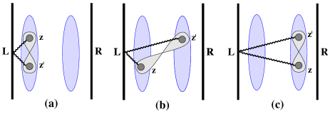
Figure 7: Contributions of the noise in the left wire to the decoherence of $\rho_{ij}(z,z^{\prime},t)$. The figures show only the coupling of one point on the wire to the atomic state. To get the total contribution to the decoherence an integration over all wire elements coupling to the atomic state has to be performed.

Instead of going into details of the derivation we will discuss the different contributions qualitatively. As the system is invariant under mirror imaging at the $\hat{y}$-$\hat{z}$-plane, corresponding to an invariance under interchange of the left (L) trap and right (R) trap label, only the following three contributions have to be distinguished (see Fig. 7).

	$J^{L}_{LL}(\zeta_{-})$	$J^{L}_{LR}(\zeta_{-})$	$J^{L}_{RR}(\zeta_{-})$
$\zeta_{-}=0$	$\frac{1}{\bar{y}_{0}^{5}}$	$\frac{2}{\bar{y}_{0}^{2}d^{3}}$	$\frac{1}{d^{5}}$
$\zeta_{-}\ll\bar{y}_{0}$	$\frac{1}{\bar{y}_{0}^{5}}$	$\frac{2}{d^{3}\bar{y}_{0}^{2}}\left(1-\frac{3}{2}\frac{\bar{y}_{0}^{2}}{d^{2}}\right)$	$\frac{1}{d^{5}}$
$\bar{y}_{0}\ll\zeta_{-}\ll d$	$\frac{4}{\bar{y}_{0}^{2}\zeta_{-}^{3}}$	$\frac{2}{d^{3}\bar{y}_{0}^{2}}\left(1-\frac{3}{2}\frac{\zeta_{-}^{2}}{d^{2}}\right)$	$\frac{1}{d^{5}}$
$d\ll\zeta_{-}$	$\frac{4}{\bar{y}_{0}^{2}\zeta_{-}^{3}}$	$\frac{2}{\zeta_{-}^{3}}\left(\frac{1}{\bar{y}_{0}^{2}}+\frac{1}{d^{2}}\right)$	$\frac{4}{d^{2}\zeta_{-}^{3}}$

Table 1: Estimate of the contributions to the decoherence. The columns for $J^{L}_{LL}$, $J^{L}_{LR}$, and $J^{L}_{RR}$ correspond to contributions (a), (b) and (c) of Fig. 7 respectively. The $J^{\gamma}_{\alpha\beta}(\zeta_{-})$ are given by Eq. (42) as a function of $\zeta_{-}=z-z^{\prime}$. The approximation assumes $\bar{y}_{0}\ll d$.

• The influence of current fluctuations in the left wire onto an atom in a state which is localized in the left arm of the trapping potential (Fig. 7a).

• The influence of current fluctuations in the left wire onto an atom which is in a superposition of a state localized in the left arm and a state localized in the right arm of the trapping potential (see Fig. 7b).

• The influence of current fluctuations in the left wire onto an atom in a state which is localized in the right arm of the trapping potential (Fig. 7c).

All other contributions are obtained by symmetry operations. Contribution (a) is given by the term proportional to $J^{L}_{LL}$ and is the dominating decoherence source in the regime $d>2\bar{y}_{0}$, as all other contributions ($J^{L}_{LR}$, $J^{L}_{RR}$ shown in the third and forth column of Table 1) are suppressed by orders of $\bar{y}_{0}/d$.

The contribution in Fig. 7b is of particular interest as it describes the cross-correlations between the noise in the left and right trapping well i.e. given by terms proportional to $J^{L}_{RL}$ and $J^{L}_{LR}$. Current fluctuations in one of the wires give rise to magnetic field fluctuations in all the trapping wells. Magnetic field fluctuations are therefore not uncorrelated. These correlations are however suppressed for $\bar{y}_{0}\ll d$ as can be seen in Table 1.

Contributions of type (c), given by terms proportional to $J^{L}_{RR}$, are the smallest contributions to decoherence as they describe the influence of the left wire current noise onto the atomic cloud in the more distant right trap. Terms of type (c) are thus negligible for wire distances $d\gg 2\bar{y}_{0}$ as the magnetic field decreases with $1/r$ and fluctuations in the trapping field are dominated by the nearest noise source i.e. contributions of type (a). In analogy to the proceeding Section III.1 we are going to approximate the transversal wavefunctions $\chi_{n}$ in Eq. (41) by 2d-HO states. However one has to be careful as this approximation holds only if the two trapping wells are sufficiently separated such that the mutual distortion of magnetic field is small. If the distance between the two traps gets close to the critical value $d=2\bar{y}_{0}$, a double-well structure arises and the harmonic approximation breaks down. We estimate the validity of the approximation by calculating the distance $d_{c}$ at which the local potential maximum, separating the two trapping wells, is of the order of the ground state energy of the isolated single trap. The trap frequency for the double-wire configuration extracted from the harmonic approximation is

$$\omega_{d}=2\omega\frac{|x_{0}|}{d}=2\omega\frac{\sqrt{d^{2}/4-\bar{y}_{0}^{2}}}{d}\;,$$ (43)

where $\omega$ is the single-wire trap frequency given in Eq. (26). Thus the ground state energy $E_{0}=\hbar\omega$ of the single-wire trap corresponds to the limit of infinite separation $d=\infty$. This energy $E_{0}$ is the maximum value for the ground state energy $\hbar\omega_{d}$ of the double-wire trap under variation of $d$. Hence $E_{0}$ is an upper bound for the ground state energy of the double well in the case $d>\bar{y}_{0}$. Using the procedure described above, we get the condition $d>\sqrt{8}\,\bar{y}_{0}$, restricting the region in which the transversal potential can be approximated as two independent 2d-HOs. The dashed line in Fig. 6 shows an example for the harmonic approximation to the trapping potential of the double-wire setup.

Performing the integration over the transverse coordinates ${\bf r}_{\perp}$, using 2d-HO states for $\chi_{n}$, gives transition matrix elements

$$\langle\delta S_{im}(z)\delta S_{nj}(z^{\prime})\rangle=4A_{0}\frac{x_{0}^{\alpha}x_{0}^{\beta}}{d^{2}}\sum_{\gamma}J^{\gamma}_{\alpha\beta}(z-z^{\prime})$$ (44)

$$\times\;\left[\tilde{\delta}_{i_{y}m_{y}}+\tilde{\delta}_{i_{x}m_{x}}\frac{\epsilon_{\alpha}y_{0}}{(x_{0}^{\alpha}+\epsilon_{\gamma}\frac{d}{2})}\right]\left[\tilde{\delta}_{n_{y}j_{y}}+\tilde{\delta}_{n_{x}j_{x}}\frac{\epsilon_{\beta}y_{0}}{(x_{0}^{\beta}+\epsilon_{\gamma}\frac{d}{2})}\right]\,,$$

where the functions $\tilde{\delta}_{ij}$ have been defined in Eq. (28). For simplicity we choose the current in the left and right wire to be the same for the derivation of Eq. (III.2).

Comparing the matrix elements obtained in Eq. (III.2) with those in Eq. (27) for the single-wire trap, we find the following differences. First of all it has to be noted that the transitions are no longer restricted to the $\hat{y}$-components of the 2d-HO. This is a direct consequence of the geometry as the positions of the trap minima are now sensitive to current fluctuations in $\hat{x}$- and $\hat{y}$-direction whereas the $\hat{x}$-position for the single-wire trap minimum was independent of the current strength in the conductor. Secondly, the prefactor of the transition matrix element in Eq. (III.2) is now a function of the spatial coordinates $x_{0}^{\alpha}$, taking the geometric changes of the trap minimum position under variation of the wire separation $d$ into account.

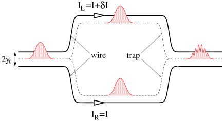
Figure 8: Schematic setup of an interferometer for cold atoms using a double-wire trap. A wavepacket is coming in from the left single waveguide formed by a double wire trap with a wire spacing of $d=2\bar{y}_{0}$. The wavepacket is split into a coherent superposition of states localized in the left and right arm of the double waveguide. Inducing a potential difference, e.g. by applying a current difference $\delta I$ in the left and right wire, gives rise to a phase shift. Remerging the wavepackets results into an interference pattern in the atom density. For a more detailed description of atom interferometers of this type see Ref. Andersson01 .

Inserting Eq. (III.2) in Eq. (21) leads to a set of equations for the dynamics of the averaged density matrix. For simplicity we restrict ourselves to the ground state and first excited state of the 2d-HO. Having in mind a spatial interferometer as suggested in Ref. Andersson01, , the most interesting quantity is the density matrix element describing the coherent superposition of a state in the left arm with a state in the right arm. Figure 8 shows the geometry of the interferometer. A wavepacket is initially prepared on the left side in a single trap. The wavepacket propagates towards the right and is split into a coherent superposition of a state in the left arm with a state in the right arm. Finally, applying a small offset between the currents in the left and right wire gives rise to a phase shift between the two wavepackets which results, after recombination, in a fringe pattern of the longitudinal density. For a more detailed description of atom interferometers of this type we refer to Andersson01 . Loss of coherence between the wavepackets in the left and right arm, due to current fluctuations in the conductors, will decrease the visibility of the interference pattern. We will thus study the decay of the components of the density matrix off-diagonal in the trap index. We will suppress the trap label (L/R) in all following expressions, bearing in mind that the left (right) index of $\rho$ will always denote a state in the left (right) trap.

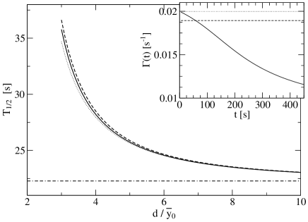
Figure 9: Decay time in the double-wire trap. $T_{1/2}$ is defined as the time it takes until $\rho_{00}^{00}(z,z^{\prime},t)$ has decayed to half of its initial value at $t=0$. The graph shows its dependence on the wire separation $d$ if all contributions in Eq. (46) are taken into account (solid line), if the cross-correlations $\beta_{i}$ are neglected (dotted line), and in the limit of $d\gg\bar{y}_{0}$, Eq. (52) (dashed line). The dash-dotted line is the $T_{1/2}$-time using the decay rate Eq. (38) for the single-wire configuration. Inset: $\Gamma(t)\equiv\ln(\rho^{00}_{00})/t$ at $d=3\bar{y}_{0}$. The trap-chip surface distance taken for the plot is $\bar{y}_{0}=10\mu\textrm{m}$ and all other trap parameters correspond to those used in Fig. 3.

We will assume that the incoming wavepacket is initially split into a symmetric superposition of the left and right arm. In addition we will choose the currents in the left and right wire to be same, $I_{L}=I_{R}$, which does not restrict the validity of the obtained result for the decoherence effects but keeps the equations simple as the full symmetry of the double-wire geometry is still conserved. The dynamics of $\rho(z,z^{\prime},t)$ is obtained from Eq. (21), leading to a matrix equation in analogy to Eq. (31) but with a density matrix vector

$${\bf{\rho}}=\left(\rho^{00}_{00},\rho^{00}_{11},\rho^{11}_{00},\rho^{01}_{10},\rho^{10}_{01}\right)\;,$$ (45)

where the upper index denotes the $\hat{x}$-state and the lower index the $\hat{y}$-state of the 2d-HO. The left (right) pair of indices refers to a state in the left (right) well. The matrix $\tilde{A}$ is

$$\tilde{A}=\left(\begin{array}[]{ccccc}\sum_{i=1}^{4}\alpha_{i}&\beta_{1}&\beta_{2}&\beta_{3}&\beta_{4}\\ \beta_{1}&\alpha_{1}+\alpha_{3}&0&\alpha_{6}&\alpha_{5}\\ \beta_{2}&0&\alpha_{2}+\alpha_{4}&\alpha_{5}&\alpha_{6}\\ \beta_{3}&\alpha_{6}&\alpha_{5}&\alpha_{1}+\alpha_{4}&0\\ \beta_{4}&\alpha_{5}&\alpha_{6}&0&\alpha_{2}+\alpha_{3}\end{array}\right).$$ (46)

Here, terms labelled by $\alpha_{i}$ are contributions of the type shown in Fig. 7a plus the corresponding term of type Fig. 7c. Terms denoted by $\beta_{i}$ are cross-correlations as described by contributions shown in Fig. 7b. The terms abbreviated as $\alpha$ do not depend on the longitudinal coordinate $z$, $z^{\prime}$ whereas the cross-correlations $\beta$ are functions of $(z-z^{\prime})$.

We will assume that the extent of the wavepacket $w_{z}$ along the trapping well is $w_{z}\ll d$. As the cross-correlations $\beta_{i}$ vary on a length scale of approximately $d$, we can replace $\beta_{i}(z-z^{\prime})$ in Eq. (46) by the constant $\beta_{i}(0)$ overest .

Further on we will assume that at $t=0$ the density matrix is given by:

$${\bf{\rho}}(t=0)=\left(\rho^{00}_{00}(t=0),0,0,0,0\right)\;.$$ (47)

Figure 9 shows the time $T_{1/2}$ it takes until $\rho^{00}_{00}(t=0)$ has decayed to half of its initial amplitude as a function of the wire separation $d$. We assume the average currents in the wires to be constant and we vary only the separation length $d$. Thus the position of the trap minima given by

$$y_{0}=\bar{y}_{0} \;,$$ (48)

$$x_{0}^{L/R}=\mp\sqrt{d^{2}/4-\bar{y}_{0}^{2}} \;,$$ (49)

move horizontally to the surface, leading to a wire-to-trap distance of

$$r_{0}=\frac{d}{\sqrt{2}}\left[1-\left(1-4\frac{y_{0}^{2}}{d^{2}}\right)^{\frac{1}{2}}\right]^{\frac{1}{2}}\;.$$ (50)

The solid line in Fig. 9 shows the $T_{1/2}$ time obtained from the solution of Eq. (31) using Eq. (46) in the approximation $\beta_{i}(z-z^{\prime})\approx\beta_{i}(0)$ for $w_{z}\ll d$. Cross-correlation terms $\beta_{i}$ play however only a minor role for the $T_{1/2}$ time as can be seen from the dotted lines in Fig. 9, showing the case where the $\beta_{i}$ terms are neglected in Eq. (46). The cross-correlation terms, shown in Fig. 7b, include terms describing positive correlation between potential fluctuations, suppressing the decoherence, but also negative correlation between potential fluctuations which enhance the decoherence. Figure 10 shows schematically the potential fluctuations $\delta V$ induced by a current fluctuation $\delta I$ in the left wire.

The inset of Fig. 9 shows the change of the decay rates over time. Taking the full matrix Eq. (46) into account (solid line) there is a change of decay rate $\Gamma_{\alpha+\beta}(t)$ towards a slower decay rate for $t\gg\Gamma_{\alpha+\beta}^{-1}(0)$. If the cross-correlations are ignored, the decay rate is constant $\Gamma_{\alpha}\approx\Gamma_{\alpha+\beta}(0)$. Inspection of $\tilde{A}$, given by Eq. (46), shows that neglecting the terms $\beta_{i}$ decouples $\rho_{00}^{00}$ from the excited states leading to an exponential decay with a single decay rate.

We finally discuss the decoherence for large distances $d$ between the wires, i.e., $d\gg\bar{y}_{0}$. For $d\gg\bar{y}_{0}$ it is sufficient to take only the influence of $\delta I_{L}$ ($\delta I_{R}$) onto the left (right) trap (given by contributions of type Fig. 7a) into account, as all other contributions are strongly suppressed by orders of $\bar{y}_{0}/d$ (see Table 1). Hence the matrix Eq. (46) decouples $\rho^{00}_{00}$ from the excited states and the remaining equation for $\rho^{00}_{00}$ can be solved analytically. The solution is

$$\rho^{00}_{00}(z,z^{\prime},t)=e^{-\Gamma t}e^{-\frac{i}{\hbar}\hat{H}t}\rho^{00}_{00}(z,z^{\prime},0)\;,$$ (51)

where $\hat{H}$ is the free Hamiltonian as defined in Section II.1. The decay rate is given as

$$\Gamma=\frac{3\pi}{2\hbar^{2}}A_{0}\frac{|x_{0}|^{2}}{d^{2}}\left[1+\frac{\bar{y}_{0}^{2}}{\left(|x_{0}|+d/2\right)^{2}}\right]\frac{1}{r_{0}^{5}}\;.$$ (52)

In the limit $d\gg\bar{y}_{0}$, Eq. (52) reduces to the decay rate obtained for the single-wire configuration, Eq.(38), shown by the dash-dotted horizontal line in Fig. 9. However, there is no spatial dependence of $\Gamma$ along the longitudinal direction $(z-z^{\prime})$ in the case of widely separated trapping wells. Plotting the $T_{1/2}$ time for the approximation given by Eq. (51) (dashed line in Fig. 9) using the decay rate Eq. (52), shows a good agreement of the approximation with the exact solution as soon as $d$ is of the order of several $\bar{y}_{0}$. Comparing all three graphs of Fig. 9 one can conclude, that the increase in $T_{1/2}$ with decreasing separation $d$ is due to geometric changes of the trap positions. An increase of the wire-to-trap distance $r_{0}$ due to a decrease of $d$, leads to an increase in the $T_{1/2}$ time as the rate of the dominating decoherence source scales with $1/r_{0}^{4}$.

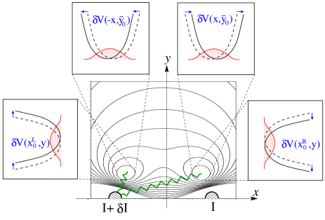
Figure 10: Influence of current fluctuations $\delta I$ in the left wire onto the potential of the trapping wells $V(x,y)=\langle S|{\bm{\mu}}|S\rangle{\bf B}$. The potential fluctuations $\delta V(x,\bar{y}_{0})=\delta V(-x,\bar{y}_{0})$ are reflection symmetric about the $\hat{y}$-$\hat{z}$-plane for $|x-x^{L/R}_{0}|\ll\bar{y}_{0}$. Hence the fluctuations in $\hat{x}$-direction are conserving the symmetry of the trapping potential. This leads to positive correlations in $\langle\delta S_{im}(z)\delta S_{nj}(z^{\prime})\rangle$ suppressing the decoherence. The fluctuation in $\hat{y}$-direction, $\delta V(x^{L}_{0},y)$, $\delta V(x^{R}_{0},y)$, show negative correlations giving rise to an increase in the decoherence rate.

IV Conclusion

Using the density-matrix formalism, we derived an equation of motion Eq. (13) to describe the consequences of current fluctuations on a cold atomic cloud in a micro-chip trap. The model allows the description of decoherence in multiple wire traps Reichel02 ; Folman01 , as well as more complex guiding systems required for the implementation of a beam splitter Cassettari01 or interference experiments Hinds01 ; Andersson01 ; Haensel03 .

The atom trap was modelled as a multi-Channel 1d-waveguide, where different channels describe different transverse modes of the waveguide. Assuming 1d-wires on the atomic chip, we examined the influence of current fluctuations along the wire onto the coherence of the atom cloud in the waveguide. We found that important contributions to the decoherence arise from transitions to neighbouring excited states.

We used this model to examine decoherence effects for two specific trapping configurations: the single-wire waveguide and the double-wire waveguide. In both configurations, decoherence of the ground state was discussed, taking processes from transitions to the first excited states into account.

The single-wire trap showed for the ground state a decoherence rate $\Gamma$ which scales with the wire-to-trap distance $r_{0}$ as $1/r_{0}^{4}$. The potential fluctuations are correlated over a length scale $r_{0}$. As a consequence the decoherence rate $\Gamma$ is a function of the relative coordinate $z-z^{\prime}$. Using trap parameters based on present experiments Folman01 we obtained decoherence rates for $r_{0}=10\mu\textrm{m}$ of the order of $\Gamma\approx 0.03\textrm{s}^{-1}$.

Extending the system to a double-wire waveguide enabled us to study decoherence for atoms in a superposition of a state localized in the left arm and a state localized in the right arm. This superposition is the basic ingredient for interference experiments. Approaching the two trapping wells, as is necessary for the splitting and merging of the wavepackets, showed a decrease in the decoherence rate. The decrease arises mostly due to geometrical rearrangements of the trap minima in the system. Cross-correlation effects proved to be of minor importance in our model. We found an explicit expression for the decoherence rate Eq. (52) in the limit of a wire-to-trap distance $r_{0}$ much smaller than the separation of the two wires $d$. This decoherence rate approaches the value for the single wire waveguide, $\Gamma=A(0)$, for decreasing $r_{0}/d$.

The decay rates extracted in this model are small for distances realized in present experiments Folman01 . However we expect that further improvement in micro-structure fabrication and trapping techniques will decrease the trap-surface distance to scales at which the decoherence from transitions to transverse states may have a considerable influence on trapped atomic clouds.

Appendix A Derivation of the projected potential correlator

This section gives a derivation of the correlation function $\langle\delta S_{im}(z)\delta S_{nj}(z^{\prime})\rangle$. A general expression of the potential fluctuation correlator $\langle\delta V({\bf x})\delta V({\bf x}^{\prime})\rangle$ for $N$ parallel traps will be derived, from which $\langle\delta S_{im}(z)\delta S_{nj}(z^{\prime})\rangle$ can be calculated using Eq. (8). Finally Eqs. (23 -25) and Eq. (41), Eq. (42) can be obtained by specifying the geometries specializing to the single and double-wire trap configurations.

The fluctuations of the trapping potential $\delta V$ is induced by current noise in the wires which gives rise to a fluctuating field $\delta{\bf B}$. The trapping potential $\delta V$ and the magnetic trapping field $\delta{\bf B}$ are linked by Eq. (1), which enables us to express $\langle\delta V({\bf x})\delta V({\bf x}^{\prime})\rangle$ in terms of magnetic field fluctuations:

$$\begin{split}\langle\delta V({\bf x})\delta V({\bf x}^{\prime})\rangle&=\sum_{ij}\langle S({\bf x})|\mu_{i}|S({\bf x})\rangle\\ &\times\;\langle S({\bf x}^{\prime})|\mu_{j}|S({\bf x}^{\prime})\rangle\langle\delta B_{i}({\bf x})\delta B_{j}({\bf x}^{\prime})\rangle\;.\end{split}$$ (53)

Thus the first step is to find the expression for $\langle\delta B_{i}({\bf x})\delta B_{j}({\bf x}^{\prime})\rangle$ as a function of the current noise. We start by calculating $\delta{\bf A}$ and $\delta{\bf B}$ using

$$\delta A_{i}({\bf x}) =\frac{\mu_{0}}{4\pi}\int d^{3}\tilde{{\bf x}}\frac{\delta j_{i}(\tilde{{\bf x}})}{|{\bf x}-\tilde{{\bf x}}|}\;,$$ (54)

$$\delta B_{i}({\bf x}) =\sum_{jk}\epsilon_{ijk}\frac{d}{dx_{j}}\delta A_{k}({\bf x})\;.$$ (55)

The current density in the set of 1d-wires is

$$\delta{\bf j}({\bf x})=\sum_{\gamma}\delta I_{\gamma}(z)\delta(x-d_{\gamma})\delta(y){\bf{\hat{z}}}\;,$$ (56)

where $d_{\gamma}$ denotes the $\hat{x}$-position of the $\gamma$-th wire. The sum over $\gamma$ reflects the fact that the total current density ${\bf j}$ is a sum of $M$ contributions to the current density arising from the set of $M$ wires. We will now insert Eq. (56) in Eq. (54) and Eq. (55) to obtain an expression for the magnetic field induced by the current in the wire array:

$$\begin{split}\delta{\bf B}({\bf x})=&\frac{\mu_{0}}{4\pi}\sum_{\gamma}\left(\begin{array}[]{c}-y\\ x-d_{\gamma}\\ 0\\ \end{array}\right)\\ \times&\int d\tilde{z}\frac{\delta I_{\gamma}(\tilde{z})}{\left[(x-d_{\gamma})^{2}+y^{2}+(z-\tilde{z})^{2}\right]^{3/2}}\;.\end{split}$$ (57)

The correlation function for the current density is now assumed to be of the form

$$\langle\delta I_{\alpha}(z)\delta I_{\beta}(z^{\prime})\rangle=4k_{\textrm{B}}T_{\textrm{eff}}\sigma A\delta(z-z^{\prime})\delta_{\alpha\beta}$$ (58)

for the reasons discussed before in Section II.3. Using Eq. (58) in combination with equations (53) and (57) gives the desired relation for the correlation function of the potential fluctuations

$$\begin{split}&\langle\delta V({\bf x})\delta V({\bf x}^{\prime})\rangle=4k_{\textrm{B}}T_{\textrm{eff}}\sigma A\left(\frac{\mu_{0}}{4\pi}\right)^{2}\\ &\times\;\sum_{\gamma}\sum_{ij}\langle S({\bf x})|\mu_{i}|S({\bf x})\rangle\langle S({\bf x}^{\prime})|\mu_{j}|S({\bf x}^{\prime})\rangle\\ &\times\;Y^{\gamma}_{ij}({\bf x},{\bf x}^{\prime})J^{\gamma}({\bf x},{\bf x}^{\prime})\;,\end{split}$$ (59)

where the following abbreviations have been introduced

$$Y^{\gamma}({\bf x},{\bf x}^{\prime})=\left(\begin{array}[]{ccc}yy^{\prime}&-y(x^{\prime}-d_{\gamma})&0\\ -(x-d_{\gamma})y^{\prime}&(x-d_{\gamma})(x^{\prime}-d_{\gamma})&0\\ 0&0&0\\ \end{array}\right)\;,$$ (60)

$$J^{\gamma}({\bf x},{\bf x}^{\prime}) = \int\limits_{-\infty}^{\infty}d\tilde{z}\left[(x-d_{\gamma})^{2}+y^{2}+(z-\tilde{z})^{2}\right]^{-\frac{3}{2}}$$ (61)

$$\left[(x^{\prime}-d_{\gamma})^{2}+y^{\prime 2}+(z^{\prime}-\tilde{z})^{2}\right]^{-\frac{3}{2}}\,.$$

Equation (61) can be further simplified if the transversal positions $x^{(\prime)}$ and $y^{(\prime)}$ are replaced by the position of the trap minimum $x_{0}^{\alpha}$ and $y_{0}^{\alpha}$ where $\alpha$ is the trap label denoting the trap in which the wavefunction is localized. The replacement of the transversal coordinates by its trap minima positions is a good approximation as the transversal widths $w$ of the trapped atomic clouds are in general much smaller than the wire-to-trap distance $r_{0}$. We have thus reduced $J^{\gamma}$ to a function which now only depends on the difference $\zeta_{-}=z-z^{\prime}$:

$$\begin{split}J^{\gamma}_{\alpha\beta}(\zeta_{-})=&\int\limits_{-\infty}^{\infty}d\tilde{z}^{\prime}\left[(x_{0}^{\alpha}-d_{\gamma})^{2}+{y_{0}^{\alpha}}^{2}+\left.\tilde{z}^{\prime}\right.^{2}\right]^{-\frac{3}{2}}\\ \times\;&\left[(x_{0}^{\beta}-d_{\gamma})^{2}+{y_{0}^{\beta}}^{2}+(\zeta_{-}-\tilde{z}^{\prime})^{2}\right]^{-\frac{3}{2}}\;,\end{split}$$ (62)

where we shifted the integration variable to $\tilde{z}^{\prime}=\tilde{z}~{}-~{}z$. Applying the formula to the single and double wire configurations leads to Eq. (25) and Eq. (42) respectively.

To obtain $\langle\delta V({\bf x})\delta V({\bf x}^{\prime})\rangle$ using Eq. (59), we still need to calculate the mean value of the atomic magnetic moment $\langle S({\bf x})|\bm{\mu}|S({\bf x})\rangle$. We assume that the magnetic moment follows the magnetic trapping field adiabatically which is reasonable as long as the Larmor precession $\omega_{L}=\mu_{B}B/\hbar$ is fast compared to the trap frequency $\omega$. Calculating the spinor $|S({\bf x})\rangle$ for an atom having spin $F=2$, either by considering the small corrections of the transversal magnetic field to $B^{(z)}_{\textrm{bias}}$ perturbatively or by calculating the rotation of the spinor as the atomic moment follows the trapping field adiabatically, results in the following expression for the spatial dependence of $|S({\bf x})\rangle$ for small deviations from the trap minimum:

$$|S({\bf x})\rangle=|2,2\rangle+\frac{B_{x}({\bf x})+iB_{y}({\bf x})}{B^{(z)}_{\textrm{bias}}}|2,1\rangle\;.$$ (63)

The spin states are denoted as $|F,m_{F}\rangle$ and the spin quantisation axis is chosen along the $\hat{z}$-axis. Making use of Eq. (63) leads to

$$\langle S({\bf x})|\bm{\mu}|S({\bf x})\rangle=2\mu_{B}g_{F}\frac{{\bf B}{({\bf x})}}{B^{(z)}_{\textrm{bias}}}\;,$$ (64)

which is an approximation to the mean value of the magnetic moment to first order in $B_{\perp}/B^{(z)}_{\textrm{bias}}$. Inserting the expression for the magnetic moment Eq. (64) into Eq. (59) and inserting the specific magnetic trapping fields for the single-wire trap, Eq. (22), or the double-wire trap, Eq. (40), we finally obtain the results for $\langle\delta S_{im}(z)\delta S_{nj}(z^{\prime})\rangle$ given by Eq. (24) for the single-wire setup and by Eq. (41) for the double-wire setup.

References

- (1) S. Chu, Rev. Mod. Phys. 70, 685 (1998); C. N. Cohen-Tannoudji, ibid., 707 (1998); W. D. Phillips, ibid., 721 (1998).
- (2) M. H. Anderson, J. R. Ensher, M. R. Matthews, C. E. Wieman, and E. A. Cornell, Science 269, 198 (1995).
- (3) K. B. Davis, M.-O. Mewes, M. R. Andrews, N. J. van Druten, D. S. Durfee, D. M. Kurn, and W. Ketterle, Phys. Rev. Lett. 75, 3969 (1995).
- (4) K. W. Madison, F. Chevy, W. Wohlleben, and J. Dalibard, Phys. Rev. Lett. 84, 806 (2000).
- (5) J. R. Abo-Shaeer, C. Raman, J. M. Vogels, and W. Ketterle, Science 292, 476 (2001).
- (6) M. R. Andrews, C. G. Townsend, H.-J. Miesner, D. S. Durfee, D. M. Kurn, and W. Ketterle, Science 275, 637 (1997).
- (7) D. Jaksch, C. Bruder, J. I. Cirac, C. W. Gardiner, and P. Zoller, Phys. Rev. Lett. 81, 3108 (1998).
- (8) M. Greiner, O. Mandel, T. Esslinger, T. W. Hänsch, and I. Bloch, Nature 415, 39 (2002).
- (9) J. D. Weinstein and K. G. Libbrecht, Phys. Rev. A 52, 4004 (1995).
- (10) J. H. Thywissen, M. Olshanii, G. Zabow, M. Drndic, K. S. Johnson, R. M. Westervelt, and M. Prentiss, Eur. Phys. J. D 7, 361 (1999).
- (11) J. Denschlag, D. Cassettari, and J. Schmiedmayer, Phys. Rev. Lett. 82, 2014 (1999).
- (12) J. Reichel, W. Hänsel, and T. W. Hänsch, Phys. Rev. Lett. 83, 3398 (1999).
- (13) D. Cassettari, B. Hessmo, R. Folman, T. Maier, and J. Schmiedmayer, Phys. Rev. Lett. 85, 5483 (2000).
- (14) W. Hänsel, J. Reichel, P. Hommelhoff, and T. W. Hänsch, Phys. Rev. Lett. 86, 608 (2001).
- (15) J. A. Sauer, M. D. Barrett, and M. S. Chapman, Phys. Rev. Lett. 87, 270401 (2002).
- (16) W. Hänsel, P. Hommelhoff, T. W. Hänsch, and J. Reichel, Nature 413, 498 (2001).
- (17) H. Ott, J. Fortagh, G. Schlotterbeck, A. Grossmann, and C. Zimmermann, Phys. Rev. Lett. 87, 230401 (2001).
- (18) S. Schneider, A. Kasper, C. vom Hagen, M. Bartenstein, B. Engeser, T. Schumm, I. Bar-Joseph, R. Folman, L. Feenstra, and J. Schmiedmayer, Phys. Rev. A 67, 023612 (2003).
- (19) A. E. Leanhardt, A. P. Chikkatur, D. Kielpinski, Y. Shin, T. L. Gustavson, W. Ketterle, and D. E. Pritchard, Phys. Rev. Lett. 89, 040401 (2002).
- (20) E. A. Hinds, C. J. Vale, and M. G. Boshier, Phys. Rev. Lett. 86, 1462 (2001).
- (21) E. Andersson, T. Calarco, R. Folman, M. Andersson, B. Hessmo, and J. Schmiedmayer, Phys. Rev. Lett. 88, 100401 (2002).
- (22) W. Hänsel, J. Reichel, P. Hommelhoff, and T. W. Hänsch, Phys. Rev. A. 64, 063607 (2001).
- (23) A. E. Leanhardt, Y. Shin, A. P. Chikkatur, D. Kielpinski, W. Ketterle, and D. E. Pritchard, Phys. Rev. Lett. 90, 100404 (2003).
- (24) J. Fortágh, H. Ott, S. Kraft, A. Günther, and C. Zimmermann, Phys. Rev. A 66, 041604(R) (2002).
- (25) S. Kraft, A. Günther, H. Ott, D. Wharam, C. Zimmermann, and J. Fortágh, J. Phys. B 35, L469 (2002).
- (26) M. P. A. Jones, C. J. Vale, D. Sahagun, B. V. Hall, and E. A. Hinds, quant-ph/0301018. (unpublished)
- (27) C. Henkel, S. Pötting, and M. Wilkens, Appl. Phys. B 69, 379 (1999).
- (28) C. Henkel and S. Pötting, Appl. Phys. B 72, 73 (2001).
- (29) C. Henkel, P. Krüger, R. Folman, and J. Schmiedmayer, Appl. Phys. B 76, 173 (2003).
- (30) A. J. Leggett, Rev. Mod. Phys. 73, 307 (2001).
- (31) J. Reichel, Appl. Phys. B 75, 469 (2002).
- (32) R. Folman, P. Krüger, J. Schmiedmayer, J. Denschlag, and C. Henkel, Adv. At. Mol. Opt. Phys. 48, 263 (2002).
- (33) C. W. Gardiner, Handbook of Stochastic Methods, (Springer, Berlin, 1998).
- (34) N. G. van Kampen, Stochastic Processes in Physics and Chemistry, (North-Holland, Amsterdam, 1990).
- (35) M. J. M. de Jong and C. W. J. Beenakker, in: Mesoscopic Electron Transport, edited by L. L. Sohn, L. P. Kouwenhoven, and G. Schön, NATO ASI Series E, Vol. 345, 225 (Kluwer Academic Publishing, Dordrecht, 1997).
- (36) Ya. M. Blanter and M. Büttiker, Phys. Rep. 336, 1 (2000).
- (37) K. E. Nagaev, Phys. Rev. B 52, 4740 (1995).
- (38) V. I. Kozub and A. M. Rudin, Phys. Rev. B 52, 7853 (1995).
- (39) The configuration studied here corresponds to the ideal case of the magnetic bias fields being perfectly aligned. Having a slight misalignment gives rise to transitions among and states of the 2d-HO.
- (40) E. Andersson, M. T. Fontenelle, and S. Stenholm, Phys. Rev. A 59, 3841 (1999).
- (41) Considering the opposite limit , we can approximate which results in -times between the solid and dotted curves in Fig. 9 depending on .