Fano resonances in the overlapping regime

Abstract

The line shape of resonances in the overlapping regime is studied by using the eigenvalues and eigenfunctions of the effective Hamiltonian of an open quantum system. A generalized expression $\tilde{q}_{k}(E)$ for the Fano parameter of the resonance state $k$ is derived that contains the interaction of the state $k$ with neighboured states $l\neq k$ via the continuum. It is energy dependent since the coupling coefficients between the state $k$ and the continuum show a resonance-like behaviour at the energies of the neighboured states $l\neq k$. Under certain conditions, the energy dependent $\tilde{q}_{k}(E)$ are equivalent to the generalized complex energy independent Fano parameters that are introduced by Kobayashi et al. in analyzing experimental data. Long-lived states appear mostly isolated from one another in the cross section, also when they are overlapped by short-lived resonance states. The $\tilde{q}_{k}(E)$ of narrow resonances allow therefore to study the complicated interplay between different time scales in the regime of overlapping resonance states by controlling them as a function of an external parameter.

The line shape of resonances is studied in many different physical systems. A resonance has a symmetrical Breit-Wigner line shape when it is far in energy from other resonances and from particle decay thresholds, and when there is no interference with any smooth background. Such a situation is seldom met in realistic systems. The interference with an energy independent background is taken into account in the approach suggested by Fano [1] for the description of autoionizing atomic states. The parametrization of the cross section can explain the asymmetry of the line shape of isolated resonances. This method was extended later to the many-channel problem and to the overlapping between broad and narrow resonances, see [2, 3] and the recent papers [4].

Deviations from the Breit-Wigner resonance form appear also when the width of the resonance state itself is energy dependent. This happens, above all, in the neighbourhood of particle decay thresholds. Under certain conditions, the Breit-Wigner resonance shape turns over even into a cusp [5]. Furthermore, the tail of bound states (with position below the first decay threshold) can be seen in the cross section at positive energy and may even interfere with resonance states lying at these positive energies [6].

Energy dependent effects may appear, however, also far from thresholds when the individual resonance states start to overlap [6]. Here, interferences between the different resonance states having different lifetimes, as well as with a smooth background may cause altogether a complicated behaviour of the cross section in the neighbourhood of the narrow resonance states. Experimental studies are performed on microwave cavities as a function of the degree of opening of the cavity [7]. In atoms, laser-induced structures are studied theoretically in the non-Hermitian Hamiltonian approach [8]. In these cases, the line shape can be controlled by means of the parameters of the laser field. A systematic experimental study is not performed, up to now.

The situation is especially complicated when the narrow resonance states are well separated from one another in the cross section and, nevertheless, overlapped by one or more broad ones and, furthermore, the cross section contains a smooth (energy-independent) part. The line shape of these resonances is studied in detail experimentally and theoretically in atoms with Rydberg series overlapped by an intruder, e.g. [9] and the textbook [3].

Another example are the neutron resonances in heavy nuclei the line shape of which is not studied, up to now. They represent a realistic example of a Gaussian orthogonal ensemble. These resonances do not decay according to an exponential law as shown theoretically [10] as well as experimentally [11]. Thus, their line shape cannot be of Breit-Wigner or Fano type with energy-independent coupling coefficients between resonance states and continuum although the resonances are well separated in energy from one another.

Recently, the line shape of resonances as well as phase jumps of the transmission amplitudes have been discussed in experiments on electron transport through mesoscopic systems [12, 13, 14, 15]. The advantage of these experiments consists in the fact that the key parameters are tuned, and the interference leading to Fano resonances is studied in greater detail. In [15], the conductance through a quantum dot in an Aharonov-Bohm interferometer is controlled by varying the strength of the magnetic field. The authors claim that the Fano parameter $q$ has to be extended to a complex number. The physical meaning of this result remains an open problem.

In order to understand the phase jumps, the effects of the signs of the dot-lead matrix elements onto the appearance of transmission zeros and the phases of the transmission amplitudes have been studied theoretically, e.g. [16, 17, 18]. These studies do not use the eigenfunctions of the Hamiltonian of the system in calculating the coupling matrix elements. Such a study is justified by the fact that the profile of the Fano resonances is independent of the special properties of the system, indeed [1]. However, the simple relation between the standard Fano parameters and the coupling coefficients between system and environment holds only in the regime of non-overlapping resonances. In the overlapping regime, the coupling coefficients are energy dependent [6, 19].

The line shape of resonances in the overlapping regime is studied in [8] for laser-induced structures in atoms. The formalism used is the effective Hamiltonian describing open quantum systems. It can be applied to the study of the resonance phenomena in the non-overlapping regime as well as in the overlapping regime [6]. The formalism of the effective Hamiltonian can be used also for the description of quantum dots. It gives reliable results not only when the dot-lead matrix elements are small but also when they are large [6, 7, 20]. An interesting feature, proven experimentally [7], is that narrow resonances appear for both small and large dot-lead (or cavity-lead) coupling coefficients. In the last case, they coexist with broad resonances and appear mostly as dips in the transmission [20, 21].

It is the aim of the present paper to study the line shape of resonances in the overlapping regime on the basis of the formalism of the effective Hamiltonian ${\cal H}$. This Hamiltonian appears in the subspace of discrete states after embedding it into the continuum (subspace of scattering states). It contains the Hamiltonian of the corresponding closed system as well as the coupling matrix elements between system and environment. It is non-Hermitian and its eigenvalues $\tilde{\cal E}_{k}$ and eigenfunctions $\tilde{\Phi}_{k}$ are complex and energy dependent. The eigenvalues provide the poles of the $S$ matrix and the eigenfunctions are used for the calculation of the coupling matrix elements between system and environment, i.e. for the numerators of the $S$ matrix in pole representation. The formalism is described in detail in the recent review [6].

In the overlapping regime, different time scales exist simultaneously due to the different crossings of the resonance states in the complex plane that are avoided, as a rule [6]. The avoided crossings can be traced, as a function of a certain parameter, in the trajectories of the eigenvalues ${\tilde{\cal E}}_{k}=\tilde{E}_{k}-\frac{i}{2}\tilde{\Gamma}_{k}$ of the non-Hermitian effective Hamiltonian ${\cal H}$. Characteristic of the motion of the poles of the $S$ matrix are the following generic results obtained for very different systems in the overlapping regime: the trajectories of the $S$ matrix poles avoid crossing with the only exception of exact crossing when the $S$ matrix has a double (or multiple) pole. At the avoided crossing, either level repulsion or level attraction occurs. The first case is caused by a predominantly real interaction between the crossing states and is accompanied by the tendency to form a uniform time scale of the system. Level attraction occurs, however, when the interaction is dominated by its imaginary part arising from the coupling via the continuum. It is accompanied by the formation of different time scales in the system: while some of the states decouple (partly) from the continuum and become long-lived (trapped), a few of the states become short-lived and wrap the long-lived ones in the cross section. The dynamics of quantum systems at high level density is determined by the interplay of these two opposite tendencies [6]. The Fano parameters reflect this interplay as will be shown in the following.

Let us recall the $S$ matrix for an isolated resonance state $k=1$ in the one-channel case,

$$S(E)=1-\,i\;\frac{\tilde{W}_{1}}{E-\tilde{\cal E}_{1}}\;.$$ (1)

Here, $\tilde{\cal E}_{1}=\tilde{E}_{1}-\frac{i}{2}\tilde{\Gamma}_{1}$ is the complex energy of the resonance state (eigenvalue of the effective Hamiltonian) and $\tilde{E}_{1}$ and $\tilde{\Gamma}_{1}$ are its position in energy and width, respectively. The $\tilde{W}_{1}$ are related to the coupling matrix elements between the resonance state and the continuum that are calculated by means of the eigenfunctions of the effective Hamiltonian. From the unitarity of the $S$ matrix follows $\tilde{W}_{1}=\tilde{\Gamma}_{1}$ for an isolated resonance state, since Eq. (1) can, in the one-resonance-one-channel case, then be written as

$$S(E) = \frac{E-{\tilde{\cal E}}_{1}^{*}}{E-{\tilde{\cal E}}_{1}}\;.$$ (2)

The $S$ matrix (2) is unitar. In the following, we assume that ${\tilde{\cal E}}_{1}$ is nearly constant inside the energy range of interest.

The unitar representation of the $S$ matrix in the one-channel case with two resonance states ($k=1,\,2$) and a smooth reaction part can be written as

$$S(E) = \exp(2i\delta)\cdot\;\frac{E-{\tilde{\cal E}}_{1}^{*}}{E-{\tilde{\cal E}}_{1}}\cdot\frac{E-{\tilde{\cal E}}_{2}^{*}}{E-{\tilde{\cal E}}_{2}}$$ (3)

$$= \exp\{2i\big{(}\delta+\delta_{1}(E)+\delta_{2}(E)\big{)}\}\;.$$ (4)

Here, $\delta$ is the phase shift related to the smooth part, and

$$\delta_{k}(E) = -\;{\rm arccot}\;\varepsilon_{k}$$ (5)

with

$$\varepsilon_{k}=\frac{2\,(E-\tilde{E}_{k})}{\tilde{\Gamma}_{k}}\,.$$ (6)

Using these expressions, the cross section reads

$$\sigma(E) = 2\,\big{(}1-{\rm Re}\,S(E)\big{)}=2\big{[}1-\cos(2\delta+2\delta_{1}(E)+2\delta_{2}(E))\big{]}$$ (7)

$$= 4\,\sin^{2}\,\big{(}\delta+\delta_{1}(E)+\delta_{2}(E)\big{)}\,.$$ (8)

In the vicinity of the energy $\tilde{E}_{1}$ of the resonance state 1 one gets from (8)

$$\sigma(E) = 4\;\big{[}\sin\eta(E)\cos\delta_{1}(E)+\sin\delta_{1}(E)\cos\eta(E)\big{]}^{2}$$ (9)

$$= 4\;\sin^{2}\eta(E)\frac{[\cot\eta(E)+\cot\delta_{1}(E)]^{2}}{\sec^{2}\delta_{1}(E)}$$ (10)

$$= 4\;\sin^{2}\eta(E)\;\frac{\big{(}\tilde{q}_{1}(E)+\varepsilon_{1}\big{)}^{2}}{\varepsilon_{1}^{2}+1}$$ (11)

where $\eta(E)\equiv\delta+\delta_{2}(E)$ and

$$\tilde{q}_{1}(E)=-\cot\eta(E)=\frac{\varepsilon_{2}\cot\delta+1}{\cot\,\delta-\varepsilon_{2}}\,.$$ (12)

Eq. (11) is the Fano representation of the cross section in the neighbourhood of the energy $\tilde{E}_{1}$ of the resonance state 1 with interference contributions from the resonance state 2 and the smooth reaction part. The Fano parameter $\tilde{q}_{1}$ is an energy dependent function. It is $\tilde{q}_{1}(E)=\varepsilon_{2}$ when $\delta\to 0$, and the energy dependence plays a role only for overlapping resonance states. For non-overlapping resonance states 1 and 2 (i.e., $\varepsilon_{2}\to\pm\infty$ at the energy $E$ of the resonance state 1) follows $\tilde{q}_{1}=-\cot\delta$ independently of $E$ in agreement with [1]. In the other extreme case of a very broad resonance state 2 ($\varepsilon_{2}\to 0$) $\tilde{q}_{1}=\tan\delta$ is also independent of $E$ but differs from the foregoing case by the additional phase $\pi/2$. It is easy to generalize (11) to include the contributions from additional resonance states ($\eta(E)=\delta+\sum_{k>1}\delta_{k}(E)$).

The energy dependence of the $\tilde{q}$ is caused by the energy dependence of the coupling coefficients between system and continuum as will be shown in the following. Assuming $\delta\to 0$, two resonance states and one common channel, the pole representation

$$S(E)=1\,-\,i\,\sum_{k=1,2}\frac{U_{k}}{E-{\tilde{\cal E}}_{k}}\$$ (13)

of the $S$ matrix can be derived from (4) in different ways.

(i) $U_{k}=W_{k}$ are energy independent,

$$W_{k} = \tilde{\Gamma}_{k}\Big{(}1-\,i\frac{\tilde{\Gamma}_{l\neq k}}{{\tilde{\cal E}}_{l\neq k}-{\tilde{\cal E}}_{k}}\Big{)}\,.$$ (14)

In deriving (14) from (3), the standard representation of the term

$$\frac{\tilde{\Gamma}_{1}\tilde{\Gamma}_{2}}{(E-\tilde{\cal E}_{1})(E-\tilde{\cal E}_{2})}=\frac{\tilde{\Gamma}_{1}\tilde{\Gamma}_{2}}{(E-\tilde{\cal E}_{1})(\tilde{\cal E}_{2}-\tilde{\cal E}_{1})}-\frac{\tilde{\Gamma}_{1}\tilde{\Gamma}_{2}}{(E-\tilde{\cal E}_{2})(\tilde{\cal E}_{2}-\tilde{\cal E}_{1})}$$

is used. The cross section reads

$$\sigma(E)=\sigma_{a1}\,\frac{(q+\varepsilon_{1})^{2}+A_{1}}{\varepsilon_{1}^{2}+1}+\sigma_{a2}\,\frac{(q+\varepsilon_{2})^{2}+A_{2}}{\varepsilon_{2}^{2}+1}+\sigma_{b}\quad$$ (15)

with the parameters

$$q = \varepsilon_{12}=\frac{2(\tilde{E}_{1}-\tilde{E}_{2})}{\tilde{\Gamma}_{1}-\tilde{\Gamma}_{2}}\qquad A_{k}=\frac{\tilde{\Gamma}_{k}}{\tilde{\Gamma}_{l\neq k}}(\varepsilon_{12}^{2}+1)+2(1-\varepsilon_{12}^{2})$$ (16)

and

$$\sigma_{ak}=\frac{4\tilde{\Gamma}_{l\neq k}}{(\tilde{\Gamma}_{k}-\tilde{\Gamma}_{l})\;(\varepsilon_{12}^{2}+1)}\qquad\sigma_{b}=\frac{4}{\varepsilon_{12}^{2}+1}$$ (17)

that are all energy independent. The parametric expression (15) for the cross section is similar to that given in [22] for the case of one resonance state coupled to several decaying channels. The parameter $q$ can be considered as Fano parameter. In our case of one resonance state coupled to another one, the contributions to each resonance state in (15) are modified by the additional term $A_{k}$. According to (17), it is $\sigma_{a1}+\sigma_{a2}+\sigma_{b}=0$, and at least one of the parameters $\sigma_{ak}$ is negative. This parameter has no physical meaning at all. The two parameters $q$ and $A_{k}$ are not defined at a double pole of the $S$ matrix since they are singular when the double pole is approached along the real energy axis. That means also the $W_{k}$ have, in this case, no physical meaning. The singularities in (16) and (17) appearing in approaching a double pole of the $S$ matrix cancel each other in the expression for the cross section.

For overlapping resonance states with $\tilde{\Gamma}_{2}\gg\tilde{\Gamma}_{1}$ and $|\tilde{E}_{1}-\tilde{E}_{2}|<\tilde{\Gamma}_{2}/2$, it holds $\varepsilon_{12}^{2}<1$. In this case, the $A_{k}$ are positive and it is possible to introduce complex energy independent Fano parameters

$$q_{k}\equiv q+iA_{k}^{1/2}$$ (18)

in the equation (15) for the cross section,

$$\sigma(E)=\sum_{k=1,2}\sigma_{ak}\frac{|q_{k}+\varepsilon_{k}|^{2}}{\varepsilon_{k}^{2}+1}+\sigma_{b}\;.$$ (19)

This is in analogy to the result obtained in [15] from the analysis of experimental data. It is also similar to an expression for the Fano parameter obtained in a completely different approach [23].

(ii) $U_{k}=\tilde{W}_{k}$ are energy dependent,

$$\tilde{W}_{k} = \tilde{\Gamma}_{k}\;\Big{(}1-\,i\,\frac{\tilde{\Gamma}_{l\neq k}}{2E-\tilde{\cal E}_{k}-\tilde{\cal E}_{l\neq k}}\Big{)}\,.\quad$$ (20)

In deriving (20), the non-standard representation of the term

$$\frac{\tilde{\Gamma}_{1}\tilde{\Gamma}_{2}}{(E-\tilde{\cal E}_{1})(E-\tilde{\cal E}_{2})}=\frac{\tilde{\Gamma}_{1}\tilde{\Gamma}_{2}}{(E-\tilde{\cal E}_{1})(2E-\tilde{\cal E}_{1}-\tilde{\cal E}_{2})}+\frac{\tilde{\Gamma}_{1}\tilde{\Gamma}_{2}}{(E-\tilde{\cal E}_{2})(2E-\tilde{\cal E}_{1}-\tilde{\cal E}_{2})}$$

is used. The $\tilde{W}_{k}$ have a physical meaning also in the overlapping regime. They are the coupling coefficients between the states of the system and the continuum that are calculated for realistic systems in the framework of a unified description of structure and reaction aspects [6], i.e. by means of the eigenfunctions of the effective Hamiltonian. As can be seen from (20), the energy dependence of $\tilde{W}_{k}$ appears due to its resonance behaviour at the energy of another resonance state $l\neq k$. This is in complete agreement with (12) for the energy dependent Fano parameter $\tilde{q}_{k}(E)$: near the energy of the resonance state 1, the cross section is given by (11) with the Fano parameter (12). Furthermore, the $S$ matrix goes over smoothly in

$$S = 1-2\,i\,\frac{\tilde{\Gamma}_{d}}{E-\tilde{E}_{d}+\,\frac{i}{2}\,\tilde{\Gamma}_{d}}-\frac{\tilde{\Gamma}_{d}^{2}}{(E-\tilde{E}_{d}+\,\frac{i}{2}\,\tilde{\Gamma}_{d})^{2}}\qquad$$ (21)

when $\tilde{E}_{1}\to\tilde{E}_{2}\equiv\tilde{E}_{d}$ and $\tilde{\Gamma}_{1}\to\tilde{\Gamma}_{2}\equiv\tilde{\Gamma}_{d}$ (double pole of the $S$ matrix, see [24]). The second term corresponds to the usual linear term while the third term is quadratic. The interference between these two parts is illustrated in Fig. 1 where the cross section is shown for the case of two resonance states with equal positions $\tilde{E}_{d}$ and widths $\tilde{\Gamma}_{d}$, coupled to one channel, for different $\delta$. The asymmetry of the line shape of both peaks is, in the case $\delta=0$ (Fig. 1.a), caused solely by the overlapping of the two resonance states. For comparison, the cross section with the two resonance states without any coupling between them is also shown in Fig. 1 (dashed curves).

The energy independent coupling coefficients $W_{k}$, Eq. (14), lose their physical meaning in the overlapping regime, since here the energy dependence of the coupling coefficients of the resonance states to the continuum can not be neglected (see [19] and [6] for numerical examples). It is different from that of the $\tilde{\Gamma}_{k}$ even in the one-channel case due to the biorthogonality of the wave functions of the resonance states [6]. Nevertheless, the two representations of the $S$ matrix (13) with energy independent $W_{k}$ and energy dependent $\tilde{W}_{k}$ are equivalent in almost all cases. At the double pole of the $S$ matrix, however, the $W_{k}$ have a singularity while the $\tilde{W}_{k}$ behave smoothly. Since $\sigma(E)=|1-S(E)|^{2}$, the energy independent Fano parameters can be expressed by $W_{k}$ and the energy dependent ones by $\tilde{W}_{k}$. That means, also the energy independent Fano parameters lose their physical meaning in the overlapping regime.

As can be seen from (12), the energy dependent Fano parameter $\tilde{q}_{k}(E)$ contains the influence from other resonance states and the background without any contribution from its own $\tilde{\Gamma}_{k}$. Also $\tilde{E}_{k}$ is not directly involved in the expression for the $\tilde{q}_{k}(E)$. The $\tilde{q}_{k}(E)$ allows therefore to analyze, in a very transparent manner, the mutial influence of resonance states in the overlapping region in the neighbourhood of the resonance state $k$. This is in contrast to the energy independent Fano parameters $q$ that are more complicated for an interpretation of the data. According to (16), they contain the contributions from neighbouring resonance states together with their own parameters.

In the multi-channel case, the matrix elements $S_{cc^{\prime}}$ are of the same structure as those given in (13) for the one-channel case. The coupling coefficients

$$U_{k}^{cc^{\prime}}=\tilde{W}_{k}^{cc^{\prime}}\equiv(\tilde{W}_{k}^{c})^{1/2}\;(\tilde{W}_{k}^{c^{\prime}})^{1/2}$$ (22)

in $S_{cc^{\prime}}$ are, generally, complex and energy dependent [6]. In the two-resonance case, the $S$ matrix elements (with $\delta=0$) are

$$S_{cc^{\prime}} = \delta_{cc^{\prime}}-i\sum_{k=1,2}\frac{(\tilde{W}_{k}^{c})^{1/2}\;(\tilde{W}_{k}^{c^{\prime}})^{1/2}}{E-{\tilde{\cal E}}_{k}}-\,i\,X_{12}^{cc^{\prime}}\,.\qquad$$ (23)

Here, the $X_{12}^{cc^{\prime}}\propto 1/\big{(}(E-{\tilde{\cal E}}_{1})(E-{\tilde{\cal E}}_{2})\big{)}$ can be parametrized by means of energy dependent as well as by energy independent parameters in the same manner as in the one-channel case. The energy independent parameters have, however, no physical meaning at all in the overlapping regime.

We discuss now the behaviour of the $\tilde{q}_{k}(E)$ in more detail. It follows immediately from (12) that $\tilde{q}_{1}(E)=0$ at the energy

$$E=\tilde{E}_{2}-\frac{1}{2}\,\tilde{\Gamma}_{2}\,\tan\,\delta\;.$$ (24)

When this condition is fulfilled in the neighbourhood of $\tilde{E}_{1}$ and $\tilde{\Gamma}_{1}\ll\tilde{\Gamma}_{2}$, then the narrow resonance state appears as a window-type resonance (dip) in the cross section ($q$ reversal [25]), see Fig. 2.a, full curve. It occurs, however, as a Breit-Wigner type resonance when

$$E=\tilde{E}_{2}+\frac{1}{2}\,\tilde{\Gamma}_{2}\,\cot\,\delta$$ (25)

is fulfilled near $\tilde{E}_{1}$, see Fig. 2.b, full curve. In Fig. 2, the narrow resonance 1 is overlapped by the broad resonance 2 ($\tilde{\Gamma}_{1}=0.1\,\tilde{\Gamma}_{2},\;\tilde{E}_{2}-\tilde{E}_{1}=0.5\,\tilde{\Gamma}_{2},\;\tilde{\Gamma}_{1}+\tilde{\Gamma}_{2}=1.1\,\tilde{\Gamma}_{2}$) and interferes with the smooth reaction part. Fig. 2 remains almost unchanged by varying $\tilde{E}_{2}$ and $\tilde{\Gamma}_{2}$ and correspondingly $\delta_{0}$, as long as $\tilde{\Gamma}_{2}\gg\tilde{\Gamma}_{1}$. We underline that the narrow resonance 1 appears in the cross section as an isolated peak in spite of the overlapping of the resonance state 1 with the broad resonance state 2. The reason is that Eq. (25) is fulfilled near the energy of the narrow resonance, but not Eq. (24), due to the interference with the smooth part.

The contour plot of the cross section (Fig. 2 bottom) shows that its resonance structure varies periodically with the phase $\delta$ of the background for fixed energies $E$. Accordingly, the asymmetry of the line shape varies between $\tilde{q}_{1}\to-\infty$ and $\tilde{q}_{1}\to+\infty$ periodically (as can be seen also directly from the analytical expression (12) for $\tilde{q}_{1}$). Such a behaviour is observed experimentally in the conductance peaks through a quantum dot as a function of the strength of the magnetic field [15] (that has obviously a small influence on the position and width of the narrow resonances). The complex Fano parameters introduced in [15] from a fit of the data, simulate the overlapping of the studied narrow resonance state by a broad resonance state and the phase dependence of $\tilde{q}_{k}(E)$ in the overlapping regime. This conclusion follows from the numerical study shown in Fig. 2 as well as from the analytical study resulting in Eqs. (18) and (19) for this case.

In both representations, Eqs. (12) and (18), the Fano parameter is generalized when applied to resonances in the overlapping regime. Both representations are equivalent in most cases. The difference between both generalizations can be seen best when applied to an analysis of the data in the vicinity of the energy of one of the resonance states. The energy independent complex parameter (18) contains the energies and widths of both resonance states, so that it is difficult to receive spectroscopic information. The energy dependent value (12), however, contains the influence of only the other resonance state allowing an analysis in a very transparent manner. This property qualifies the energy dependent Fano parameter (12) for the description of resonances in the overlapping regime. We underline, however, that the $\tilde{q}_{k}(E)$ are not suitable for the parametrization of the cross section around a double pole of the $S$ matrix due to the quadratic term appearing in (21). Here, the cross section can be parametrized as $\sigma(E)=16\cos^{2}\delta[(\tilde{q}_{d}(E)+\varepsilon_{d})^{2}/(\varepsilon_{d}^{2}+1)^{2}]$ with $\tilde{q}_{d}(E)=\frac{1}{2}(1-\varepsilon_{d}^{2})\tan\delta$ and $\varepsilon_{1}\to\varepsilon_{2}\equiv\varepsilon_{d}$.

It would be interesting to look for the broad resonance state(s) and to study its (their) influence on other narrow resonances in detail. According to our study, the broad resonance may exist in the arm or it may coexist with the narrow resonances in the quantum dot itself. The last possibility can not be excluded theoretically. Quite on the contrary, it corresponds to the results obtained for other small quantum systems where resonance states (eigenstates of the effective Hamiltonian) of very different lifetimes are known to coexist [6]. An experimental study of this question would allow to see generic features of open quantum systems also in quantum dots. Furthermore, results from the interference between two resonance states in the very neighbourhood of a double pole of the $S$ matrix (that can be studied in a symmetrical device with two quantum dots) will prove the resonance scenario described by an effective Hamiltonian as discussed in the present paper.

Summarizing, we conclude that the line shape of narrow resonances in the overlapping regime contains information on generic properties of open quantum systems. One of these properties is the existence of different time scales that are involved in the eigenvalues and eigenfunctions of the effective Hamiltonian of the system. A control by external parameters allows to trace their formation by opening the system and to study their interesting interplay. A direct experimental study of the generic resonance features in, e.g., atomic nuclei is difficult due to the strong residual interaction between the participating particles in nuclei. Quantum dots are much more suitable for such a study due to the flexibility in controlling the system by means of different external parameters. Further experimental as well as theoretical studies are highly desirable for both a better understanding of generic properties of open quantum systems and the construction of quantum dots with special properties.

We are indebted to J.M. Rost for valuable discussions. A.I.M. gratefully acknowledges the hospitality of the Max-Planck-Institut für Physik komplexer Systeme.

FIG. 1.: The cross section in the neighbourhood of a double pole of the $S$ matrix ($\tilde{E}_{1}=\tilde{E}_{2}$ and $\tilde{\Gamma}_{1}=\tilde{\Gamma}_{2}$). The direct scattering phase $\delta$ is: (a) $\delta=0$, (b) $\delta=\frac{1}{4}\pi$, (c) $\delta=\frac{1}{2}\pi$, (d) $\delta=\frac{3}{4}\pi$. The dashed curves correspond to the case of the two resonance states without any interaction between them.

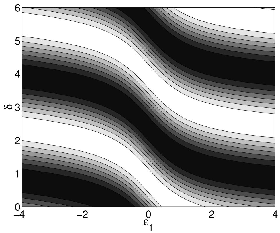
FIG. 2.: The cross section in the vicinity of the resonance 1 for $\tilde{\Gamma}_{1}=0.1\,\tilde{\Gamma}_{2},\;\tilde{E}_{2}-\tilde{E}_{1}=0.5\,\tilde{\Gamma}_{2}$. Top: (a) $\delta=\delta_{0}=-{\rm arctan}\,\varepsilon_{2}(E=\tilde{E}_{1})$ (full curve), $\delta=\delta_{0}-0.5$ (dashed curve), $\delta=\delta_{0}+0.5$ (dotted curve). (b) The same as in (a), but $\delta_{0}={\rm arccot}\,\varepsilon_{2}(E=\tilde{E}_{1})$. Bottom: The contour plot of the cross section.

REFERENCES

- [1] U. Fano, Phys. Rev. 124, 1866 (1961)
- [2] F.N. Mies, Phys. Rev. 175, 164 (1968)
- [3] H. Friedrich, Theoretical Atomic Physics, Springer 1990
- [4] E. Narevicius and N. Moiseyev, Phys. Rev. Lett. 81, 2221 (1998); Ph. Durand and I. Paidarova, J. Phys. B 35, 469 (2002); M.M. Tabanli, J.L. Peacher, and D.H. Madison, J. Phys. B 36, 217 (2003)
- [5] I. Rotter, Rep. Progr. Phys. 54, 635 (1991)
- [6] J. Okołowicz, M. Płoszajczak, and I. Rotter, Phys. Reports 374, 271 (2003)
- [7] E. Persson, I. Rotter, H.J. Stöckmann, and M. Barth, Phys. Rev. Lett. 85, 2478 (2000); H.J. Stöckmann, E. Persson, Y.H. Kim, M. Barth, U. Kuhl, and I. Rotter, Phys. Rev. E 65, 066211 (2002)
- [8] A. I. Magunov, I. Rotter, and S. I. Strakhova, J. Phys. B 32, 1489 (1999); 32, 1669 (1999); 34, 29 (2001)
- [9] J.P. Connerade, A.M. Lane, M.A. Baig, J. Phys. B 18, 3507 (1985); M.A. Baig, J.P. Connerade, J. Phys. B 18, 3487 (1985); M.A. Baig, S. Ahmad, J.P. Connerade, W. Dussa, and J. Hormes, Phys. Rev. A 45, 7963 (1992)
- [10] H.L. Harney, F.M. Dittes and A. Müller, Ann. Phys. (N.Y.) 220, 159 (1992); F.M. Dittes, Phys. Rep. 339, 215 (2000)
- [11] H. Alt, H.D. Gräf, H.L. Harney, R. Hofferbert, H. Lengeler, A. Richter, P. Schardt, and H.A. Weidenmüller, Phys. Rev. Lett. 74, 62 (1995)
- [12] A. Yacoby, M. Heiblum, D. Mahalu, and H. Shtrikman, Phys. Rev. Lett. 74, 4047 (1995); E. Buks, R. Schuster, M. Heiblum, D. Mahalu, V. Umansky, and H. Shtrikman, Phys. Rev. Lett. 77, 4664 (1996); R. Schuster, E. Buks, M. Heiblum, D. Mahalu, V. Umansky, and H. Shtrikman, Nature (London) 385, 417 (1997).
- [13] V. Madhavan, W. Chen, T. Jamneala, M.F. Crommie, and N.S. Wingreen, Science 280, 567 (1998)
- [14] J. Göres, D. Goldhaber-Gordon, S. Heemeyer, M. A. Kastner, H. Shtrikman, D. Mahalu, and U. Meirav, Phys. Rev. B 62, 2188 (2000)
- [15] K. Kobayashi, H. Aikawa, S. Katsumoto, and Y. Iye, Phys. Rev. Lett. 88, 256806 (2002)
- [16] A. Silva, Y. Oreg and Y. Gefen, Phys. Rev. B 66, 195316 (2002).
- [17] A. Aharony, E. Entin-Wohlmann, B.I. Halperin, and Y. Imry, Phys. Rev. B 66, 115311 (2002)
- [18] T.S. Kim and S. Hershfield, cond-mat/0211525 (November 2002)
- [19] I. Rotter, quant-ph/0304197 (April 2003)
- [20] A.F. Sadreev and I. Rotter, quant-ph/0304147 (April 2003)
- [21] R.G. Nazmitdinov, K.N. Pichugin, I. Rotter and P. Seba, Phys. Rev. E 64, 056214 (2001); R.G. Nazmitdinov, K.N. Pichugin, I. Rotter and P. Seba, Phys. Rev. B 66, 085322 (2002)
- [22] U. Fano and J.W. Cooper, Phys. Rev. 137, 1364 (1965)
- [23] W. Hofstetter, J. König, and H. Schoeller, Phys. Rev. Lett. 87, 156803 (2001)
- [24] R.G. Newton, Scattering Theory of Waves and Particles, Springer, New York, 1982
- [25] A.M. Lane, J. Phys. B 17, 2213 (1984); 18, 2339 (1985)