Entangling power of the quantum baker’s map

Abstract

We investigate entanglement production in a class of quantum baker’s maps. The dynamics of these maps is constructed using strings of qubits, providing a natural tensor-product structure for application of various entanglement measures. We find that, in general, the quantum baker’s maps are good at generating entanglement, producing multipartite entanglement amongst the qubits close to that expected in random states. We investigate the evolution of several entanglement measures: the subsystem linear entropy, the concurrence to characterize entanglement between pairs of qubits, and two proposals for a measure of multipartite entanglement. Also derived are some new analytical formulae describing the levels of entanglement expected in random pure states.

I Introduction

The introduction of “toy” mappings that demonstrate essential features of nonlinear dynamics has led to many insights in the field of classical chaos. A well known example is the so-called baker’s transformation lichtenberg . It maps the unit square, which can be thought of as a toroidal phase space, onto itself in an area-preserving way. Interest in the baker’s map stems from its straightforward characterization in terms of a Bernoulli shift on the binary sequence that specifies a point in the unit square. It seems natural to consider a quantum version of the baker’s map for the investigation of quantum chaos. There is, however, no unique procedure for quantizing a classical map; hence, different quantum maps can lead to the same classical baker’s transformation.

Balazs and Voros balazs were the first to formulate a quantum version of the baker’s map. This was done with the help of the discrete quantum Fourier transform. Subsequently, improvements to the Balazs-Voros quantization were made by Saraceno saraceno , an optical analogy was found hannay , a canonical quantization was devised rubin ; lesniewski , and quantum computing realizations were proposed schack2 ; brun . A related quantum baker’s mapping on the sphere has also been defined pakonski .

More recently, an entire class of quantum baker’s maps, based on the $2^{N}$-dimensional Hilbert space of $N$ qubits, was proposed by Schack and one of us schack . The qubit structure provides a connection to the binary representation of the classical baker’s map. This connection comes through the use of partial Fourier transforms, which are used to define orthonormal basis states that are localized on the unit-square phase space. The $n$-th partial Fourier transform, which acts on $N-n$ of the qubits, defines orthonormal states that are localized at a lattice of phase-space points specified by $n$ position bits and $N-n$ momentum bits. Each state is localized strictly within a position width $1/2^{n}$ and roughly within a momentum width $1/2^{N-n}$. The $n$-th quantum baker’s map in the class takes the states defined by the $n$-th partial Fourier transform to the states defined by the $(n-1)$-th partial Fourier transform. This action decreases the number of position bits by one, while increasing the number of momentum bits by one, thus mimicking the stretching and squeezing of the classical baker’s map. By using this procedure, one obtains $N$ different quantum baker’s maps, one map for each number of initial position bits (or initial momentum bits). The Balazs-Voros quantization is but one member of this class, corresponding to a single initial position bit ($n=1$). The map at the other extreme ($n=N$), which has no initial momentum bits, is easily shown to be unentangling.

The classical limit of this class of baker’s maps has been investigated by two groups soklakov ; tracy . Tracy and one of us tracy found that if the number of initial momentum bits is allowed to approach infinity as the overall number of qubits goes to infinity, the classical baker’s map is recovered. This result is consistent with the findings of Soklakov and Schack soklakov . In contrast, if the number of momentum bits is held constant as the number of qubits increases to infinity, a stochastic variation of the classical baker’s map is created tracy . The simplest such limit, which holds the number of initial momentum bits constant at zero ($n=N$), follows a sequence of completely unentangling quantum baker’s maps.

Our curiosity now poses the following two questions. What is the entangling power of all the quantum baker’s maps? And what role, if any, does entanglement play in the the classical limit? This paper focuses, for the most part, on the first of these questions, investigating the entangling power of the Schack-Caves class of quantum baker’s maps. Previous investigations of entanglement in quantized chaotic systems, for the most part, have dealt with the correlations induced by coupling two or more independent systems together sakagami ; tanaka ; furuya ; angelo ; miller ; lakshminarayan ; bandyopadhyay ; tanaka2 ; fujisaki ; lahiri . Our approach here is quite different: each of our quantum baker’s maps lives in a Hilbert space with a qubit tensor-product structure; strings of qubits form a natural basis, anchoring Hilbert space to the corresponding classical phase space, and the quantum dynamics of our baker’s maps is defined explicitly in terms of this connection. We therefore expect an intimate relationship between the dynamics and the multipartite entanglement induced amongst the qubits. Using different approaches, the dynamics of entanglement in qubit bases was recently investigated in lakshminarayan2 ; bettelli .

In order to calibrate the entanglement produced by the quantum baker’s map, we compare it with the entanglement of random pure states drawn from the appropriate Hilbert space. Thus a by-product of our investigation is to derive some new exact formulae describing the levels of entanglement expected in random pure states. As measures of entanglement, we examine in detail the subsystem linear entropy, deriving formulae for the variance and third cumulant, and two proposals for a multipartite entanglement measure, where formulae for the mean and variance are given. Pairwise (mixed-state) entanglement between two qubits drawn from $N$ qubits is investigated numerically, using the concurrence as the entanglement measure.

The paper is organized as follows. In Sec. II, we introduce the baker’s map, both in classical and quantal form. Section III is devoted to discussing the measures of entanglement and the entanglement of typical pure states. In Sec. IV we explore the entangling power of the quantum baker’s maps. Finally, in Sec. V, we provide a brief discussion of our results.

II The quantum baker’s map

The classical baker’s map is a standard example of chaotic dynamics lichtenberg . It is a symplectic map of the unit square onto itself defined by

$$q_{n+1} = 2q_{n}-\lfloor 2q_{n}\rfloor\;,$$ (1)

$$p_{n+1} = \left(p_{n}+\lfloor 2q_{n}\rfloor\right)/2\;,$$ (2)

where $q,p\in[0,1)$, $\lfloor x\rfloor$ is the integer part of $x$, and $n$ denotes the $n$-th iteration of the map. Geometrically, the map stretches the unit square by a factor of two in the $q$ direction, squeezes by a factor of a half in the $p$ direction, and then stacks the right half onto the left.

Interest in the baker’s map is due mainly to the simplicity of its symbolic dynamics. If each point of the unit square is identified through its binary representation, $q=0\!\cdot\!s_{1}s_{2}\ldots=\sum_{k=1}^{\infty}s_{k}2^{-k}$ and $p=0\!\cdot\!s_{0}s_{-1}\ldots=\sum_{k=0}^{\infty}s_{-k}2^{-k-1}$ ($s_{i}\in\{0,1\}$), with a bi-infinite symbolic string

$$s=\ldots s_{-2}s_{-1}s_{0}\bullet s_{1}s_{2}s_{3}\ldots\;,$$ (3)

then the action of the baker’s map is to shift the position of the dot by one point to the right,

$$s\rightarrow s^{\prime}=\ldots s_{-2}s_{-1}s_{0}s_{1}\bullet s_{2}s_{3}\ldots\;.$$ (4)

For a quantum-mechanical version of the map, we work in a $D$-dimensional Hilbert space, ${\cal H}_{D}$, spanned by either the position states $|q_{j}\rangle$, with eigenvalues $q_{j}=(j+\beta)/D$, or the momentum states $|p_{k}\rangle$, with eigenvalues $p_{k}=(k+\alpha)/D$ ($j,k=0,\ldots,D-1$). The constants $\alpha,\beta\in[0,1)$ determine the periodicity of the space: $|q_{j+D}\rangle=e^{-2\pi i\alpha}|q_{j}\rangle$, $|p_{k+D}\rangle=e^{2\pi i\beta}|p_{k}\rangle$. Such double periodicity identifies ${\cal H}_{D}$ with a toroidal phase space. Periodic boundary conditions correspond to $\alpha=\beta=0$, and anti-periodic boundary conditions to $\alpha=\beta=1/2$; because of other symmetry considerations, these are the only two cases of interest. The vectors of each basis are orthonormal, $\langle q_{j}|q_{k}\rangle=\langle p_{j}|p_{k}\rangle=\delta_{jk}$, and the two bases are related via the finite Fourier transform,

$$\langle q_{j}|\hat{F}_{D}|q_{k}\rangle\equiv\langle q_{j}|p_{k}\rangle=\frac{1}{\sqrt{D}}\,e^{iq_{j}p_{k}/\hbar}\;.$$ (5)

For consistency of units, we must have $2\pi\hbar D=1$.

The first work on a quantum baker’s map was done by Balazs and Voros balazs . Assuming an even-dimensional Hilbert space with periodic boundary conditions, they defined a quantum baker’s map in terms of the unitary operator $\hat{B}$ that executes a single iteration of the map. To define the Balazs-Voros unitary operator in our notation, imagine that the even-dimensional Hilbert space is a tensor product of a qubit space and the space of a ($D/2$)-dimensional system. Writing $j=x(D/2)+j^{\prime}$, $x\in\{0,1\}$, we can write the position eigenstates as $|q_{j}\rangle=|x\rangle\otimes|j^{\prime}\rangle$, where the states $|x\rangle$ make up the standard basis for the qubit, and the states $|j^{\prime}\rangle$ are a basis for the ($D/2$)-dimensional system. The state of the qubit thus determines whether the position eigenstate lies in the left or right half of the unit square. The Balazs-Voros quantum baker’s map is defined by

$$\hat{B}=\hat{F}_{D}\circ\Bigl{(}\hat{1}_{2}\otimes\hat{F}_{D/2}^{-1}\Bigr{)}\;,$$ (6)

where $\hat{1}_{2}$ is the unit operator for the qubit, and $\hat{F}_{D/2}$ is the finite Fourier transform on the ($D/2$)-dimensional system. The unitary $\hat{B}$ does separate inverse Fourier transforms on the left and right halves of the unit square, followed by a full Fourier transform. Later Saraceno saraceno improved certain symmetry characteristics of this quantum baker’s map by using anti-periodic boundary conditions.

Taking again the anti-periodic Hilbert space (which we use throughout the remainder of this paper), Schack and one of us schack introduced a class of quantum baker’s maps for dimensions $D=2^{N}$. For these cases, we can model our Hilbert space as the the space of $N$ qubits, and the position states can be defined as product states for the qubits in the standard basis, i.e.,

$$|q_{j}\rangle=|x_{1}\rangle\otimes|x_{2}\rangle\otimes\cdots\otimes|x_{N}\rangle\;,$$ (7)

where $j$ has the binary expansion

$$j=x_{1}\ldots x_{N}\!\cdot\!0=\sum_{l=1}^{N}x_{l}2^{N-l}$$ (8)

and $q_{j}=(j+1/2)/D=0\!\cdot\!x_{1}\ldots x_{N}1$.

The connection with the classical baker’s map derives from the symbolic dynamics. The bi-infinite strings (3) that specify points in the unit square are replaced by sets of orthogonal quantum states created through the use of a partial Fourier transform

$$\hat{G}_{n}\equiv\hat{1}_{2^{n}}\otimes\hat{F}_{2^{N-n}}\;,\qquad n=0,\ldots,N,$$ (9)

where $\hat{1}_{2^{n}}$ is the unit operator on the first $n$ qubits and $\hat{F}_{2^{N-n}}$ is the Fourier transform on the remaining qubits. The partial Fourier transform thus transforms the $N-n$ least significant qubits of a position state,

$$\hat{G}_{n}\,|x_{1}\rangle\otimes\cdots\otimes|x_{n}\rangle\otimes|a_{1}\rangle\otimes\cdots\otimes|a_{N-n}\rangle=\,|x_{1}\rangle\otimes\cdots\otimes|x_{n}\rangle\otimes\frac{1}{\sqrt{2^{N-n}}}\sum_{x_{n+1},\ldots,x_{N}}|x_{n+1}\rangle\otimes\cdots\otimes|x_{N}\rangle e^{2\pi iax/2^{N-n}}\;,$$ (10)

where $a$ and $x$ are defined through the binary representations $a=a_{1}\ldots a_{N-n}\!\cdot\!1$ and $x=x_{n+1}\ldots x_{N}\!\cdot\!1$. In the limiting cases, we have $\hat{G}_{0}=\hat{F}_{D}$ and $\hat{G}_{N}=i\hat{1}$. The analogy to the classical case is made clear by introducing the following notation for the partially transformed states:

$$|\,a_{N-n}\ldots a_{1}\bullet x_{1}\ldots x_{n}\rangle\,\equiv\,\hat{G}_{n}\,\,|x_{1}\rangle\otimes\cdots\otimes|x_{n}\rangle\otimes|a_{1}\rangle\otimes\cdots\otimes|a_{N-n}\rangle\;.$$ (11)

For each value of $n$, these states form an orthonormal basis and are localized in both position and momentum. The state $|a_{N-n}\ldots a_{1}\bullet x_{1}\ldots x_{n}\rangle$ is strictly localized in a position region of width $1/2^{n}$ centered at $0\!\cdot\!x_{1}\ldots x_{n}1$ and is roughly localized in a momentum region of width $1/2^{N-n}$ centered at $0\!\cdot\!a_{1}\ldots a_{N-n}1$. In the notation of Eq. (3), it is localized at the phase-space point $1a_{N-n}\ldots a_{1}\bullet x_{1}\ldots x_{n}1$. Notice that $|a_{N}\ldots a_{1}\bullet\rangle=\hat{G}_{0}\,|a_{1}\rangle\otimes\cdots\otimes|a_{N}\rangle$ is a momentum eigenstate and that $|\!\bullet x_{1}\ldots x_{N}\rangle=\hat{G}_{N}\,|x_{1}\rangle\otimes\cdots\otimes|x_{N}\rangle=\,i|x_{1}\rangle\otimes\cdots\otimes|x_{N}\rangle$ is a position eigenstate, the $i$ being a consequence of the anti-periodic boundary conditions.

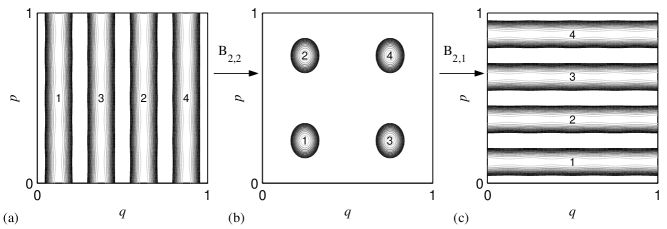
Figure 1: Husimi function for each partially Fourier transformed state (11) when $N=2$: (a) $n=2$, (b) $n=1$, and (c) $n=0$. The action of the quantum baker’s map $\hat{B}_{2,2}$ is to map the four states in (a) to the four states in (b), as shown by the numbers labeling the states. Similarly, the action of $\hat{B}_{2,1}$ is to map the states in (b) to the states in (c).

Using this notation, a quantum baker’s map on $N$ qubits is defined for each value of $n=1,\ldots,N$ by the single-iteration unitary operator schack

$$\hat{B}_{N,n}\,\equiv\,\hat{G}^{\phantom{-1}}_{n-1}\circ\hat{S}_{n}\circ\hat{G}^{\,-1}_{n}\;=\sum_{x_{1},\dots,x_{n}}\sum_{a_{1},\dots,a_{N-n}}|\,a_{N-n}\dots a_{1}x_{1}\bullet x_{2}\dots x_{n}\rangle\langle a_{N-n}\dots a_{1}\bullet x_{1}x_{2}\dots x_{n}|\;,$$ (12)

where the shift operator $\hat{S}_{n}$ acts only on the first $n$ qubits, i.e., $\hat{S}_{n}|x_{1}\rangle\otimes|x_{2}\rangle\otimes\cdots\otimes|x_{n}\rangle\otimes|x_{n+1}\rangle\otimes\cdots\otimes|x_{N}\rangle=|x_{2}\rangle\otimes\cdots\otimes|x_{n}\rangle\otimes|x_{1}\rangle\otimes|x_{n+1}\rangle\otimes\cdots\otimes|x_{N}\rangle$. Notice that since $\hat{S}_{n}$ commutes with $\hat{G}_{n}^{\,-1}$, we can put $\hat{B}_{N,n}$ in the form

$$\hat{B}_{N,n}=\hat{1}_{2^{n-1}}\otimes\Bigl{(}\hat{F}_{2^{N-n+1}}\circ(\hat{1}_{2}\otimes\hat{F}_{2^{N-n}}^{-1})\Bigr{)}\circ\hat{S}_{n}\;.$$ (13)

Since $\hat{S}_{1}$ is the unit operator, it is clear that $\hat{B}_{N,1}$ is the Balazs-Voros-Saraceno quantum baker’s map (6).

We can also write

$$\hat{B}_{N,n}=\hat{1}_{2^{n-1}}\otimes\hat{B}_{N-n+1,1}\circ\hat{S}_{n}\;,$$ (14)

which shows that the action of $\hat{B}_{N,n}$ is a shift of the $n$ leftmost qubits followed by application of the Balazs-Voros-Saraceno baker’s map to the $N-n+1$ rightmost qubits. At each iteration, the shift map $\hat{S}_{n}$ does two things: it shifts the $n$-th qubit, the most significant qubit that was subject to the previous application of $\hat{B}_{N-n+1,1}$, out of the region subject to the next application of $\hat{B}_{N-n+1,1}$, and it shifts the most significant (first) qubit into the region of subsequent application of $\hat{B}_{N-n+1,1}$.

The quantum baker’s map $\hat{B}_{N,n}$ takes a state localized at $1a_{N-n}\ldots a_{1}\bullet x_{1}\ldots x_{n}1$ to a state localized at $1a_{N-n}\ldots a_{1}x_{1}\bullet x_{2}\ldots x_{n}1$. The decrease in the number of position bits and increase in momentum bits enforces a stretching and squeezing of phase space in a manner resembling the classical baker’s map. In Fig. 1(a), (b), and (c), we plot the Husimi function (defined as in tracy ) for the partially Fourier transformed states (11) when $N=2$, and $n=2$, 1 and 0, respectively. The quantum baker’s map is a one-to-one mapping of one basis to another, as shown in the figure.

One useful representation of our quantum baker’s maps, introduced in schack , starts from using standard techniques nielsenchuang to write the partially transformed states (10) as product states:

$$|\,a_{N-n}\ldots a_{1}\bullet x_{1}\ldots x_{n}\rangle\,=\,e^{\pi i(0\!\cdot\!a_{1}\ldots a_{N-n}1)}\Biggl{(}\,\bigotimes_{k=1}^{n}|x_{k}\rangle\Biggr{)}\Biggl{(}\,\bigotimes_{k=n+1}^{N}{1\over\sqrt{2}}\Bigl{(}|0\rangle+e^{2\pi i(0\!\cdot\!a_{N-k+1}\ldots a_{N-n}1)}|1\rangle\Bigr{)}\Biggr{)}\;.$$ (15)

These input states are mapped by $\hat{B}_{N,n}$ to output states

$$|\,a_{N-n}\ldots a_{1}x_{1}\bullet x_{2}\ldots x_{n}\rangle\,=\, e^{\pi i(0\!\cdot\!x_{1}a_{1}\ldots a_{N-n}1)}\Biggl{(}\,\bigotimes_{k=2}^{n}|x_{k}\rangle\Biggr{)}$$

$$\quad\Biggl{(}\,\bigotimes_{k=n+1}^{N}{1\over\sqrt{2}}\Bigl{(}|0\rangle+e^{2\pi i(0\!\cdot\!a_{N-k+1}\ldots a_{N-n}1)}|1\rangle\Bigr{)}\Biggr{)}\otimes{1\over\sqrt{2}}\Bigl{(}|0\rangle+e^{2\pi i(0\!\cdot\!x_{1}a_{1}\ldots a_{N-n}1)}|1\rangle\Bigr{)}\;.$$

These forms show that the quantum baker’s map $\hat{B}_{N,n}$ shifts the states of all the qubits to the left, except the state of the leftmost, most significant qubit. The state $|x_{1}\rangle$ of the leftmost qubit can be thought of as being shifted to the rightmost qubit, where it suffers a controlled phase change that is determined by the state parameters $a_{1},\ldots,a_{N-n}$ of the original “momentum qubits.” The quantum baker’s map can thus be written as a shift map on a finite string of qubits, followed by a controlled phase change on the least significant qubit. Soklakov and Schack soklakov have developed this shift representation into a useful tool. Using an approach based on coarse graining in this representation, they investigated the classical limit of the quantum baker’s maps.

Another useful representation of our quantum baker’s maps is the qubit (position) representation

$$\hat{B}_{N,n}=\frac{\sqrt{2}}{2^{N-n+1}}\!\!\!\!\sum_{\begin{array}[]{c}\scriptstyle x_{1},\dots,x_{n}\\ \scriptstyle a_{1},\dots,a_{N-n}\end{array}}\!\!\sum_{\begin{array}[]{c}\scriptstyle y_{1},\dots,y_{N-n}\\ \scriptstyle z_{1},\dots,z_{N-n+1}\end{array}}\!\!\!\! |x_{2}\rangle\langle x_{1}|\otimes\cdots\otimes|x_{n}\rangle\langle x_{n-1}|\otimes|z_{1}\rangle\langle x_{n}|\otimes|z_{2}\rangle\langle y_{1}|\otimes\cdots\otimes|z_{N-n+1}\rangle\langle y_{N-n}|$$

$$\times\exp\!\left[\frac{\pi i}{2^{N-n}}\Big{(}(j+1/2)(l+1/2)+2^{N-n}x_{1}(l+1/2)-2(j+1/2)(k+1/2)\Big{)}\right]\;,$$

where

$$j=\sum_{k=1}^{N-n}a_{k}2^{N-n-k}\text{,}\quad k=\sum_{k=1}^{N-n}y_{k}2^{N-n-k}\text{,}\quad\text{and}\quad l=\sum_{k=1}^{N-n+1}z_{k}2^{N-n+1-k}.$$

Soklakov and Schack soklakov have found simplified forms of this qubit representation, suitable for asymptotic analysis of the classical limit.

The classical limit for the above quantum baker’s maps has also been investigated in tracy , using an analysis based on the limiting behavior of the coherent-state propagator of $\hat{B}_{N,n}$. When $D=2^{N}\rightarrow\infty$, the total number of qubits $N$ necessarily becomes infinite, but one has a considerable choice in how to take this limit. For example, we could use only one position bit, thus fixing $n=1$, and let the number of momentum bits $N-1$ become large. This is the limiting case of the Balazs-Voros-Saraceno quantization. There is, however, a wide variety of other scenarios to consider, e.g., $n=N/2$ or $n=2N/3-1$ as $N\rightarrow\infty$. In tracy it was shown that provided the number of momentum bits $N-n$ approaches infinity, the correct classical behavior is recovered in the limit. If the number of momentum bits remains constant, e.g., $n=N$ as $N\rightarrow\infty$, a stochastic variant of the classical baker’s map is found. These results are consistent with those obtained previously by Soklakov and Schack soklakov .

The special case $n=N$, which does not limit to the classical baker’s map, has other interesting properties. Although all finite-dimensional unitary operators are quasi-periodic, the quantum baker’s map $\hat{B}_{N,N}$ is strictly periodic,

$$\hat{B}_{N,N}^{\,4N}=1\;,$$ (23)

as we show below. All its eigenvalues, therefore, are $4N$-th roots of unity, i.e., of the form $e^{\pi ik/2N}$, and, hence, there are degeneracies when $N>4$. This represents a strong deviation from the predictions of random matrix theory haake ; guhr ; brody . The property (23) can be easily shown by noting that $\hat{B}_{N,N}=-i\hat{G}_{N-1}\circ\hat{S}_{N}=-i(\hat{1}_{2^{N-1}}\otimes\hat{F}_{2})\circ\hat{S}_{N}$; i.e., $\hat{B}_{N,N}$ is a shift followed by application of the unitary

$$\hat{U}\equiv-i\hat{F}_{2}={1\over\sqrt{2}}\Bigl{(}e^{-\pi i/4}(|0\rangle\langle 0|+|1\rangle\langle 1|)+e^{\pi i/4}(|0\rangle\langle 1|+|1\rangle\langle 0|)\Big{)}=e^{-\pi i/4}e^{i\hat{\sigma}_{x}(\pi/4)}$$ (24)

to the least significant qubit. On product states, the action of $\hat{B}_{N,N}$ can be written explicitly as

$$\hat{B}_{N,N}|\psi_{1}\rangle\otimes|\psi_{2}\rangle\otimes\dots\otimes|\psi_{N}\rangle=|\psi_{2}\rangle\otimes\dots\otimes|\psi_{N}\rangle\otimes\hat{U}|\psi_{1}\rangle\;.$$ (25)

Since $\hat{U}_{1}^{4}=1$, we get the property (23). One can now also see that $\hat{B}_{N,N}$ cannot entangle initial product states.

The eigenstates of $\hat{U}$ are $(|0\rangle+|1\rangle)/\sqrt{2}$, with eigenvalue $+1$, and $(|0\rangle-|1\rangle)/\sqrt{2}$, with eigenvalue $-i$. For the discussion in this paragraph, label these eigenstates by their eigenvalues $\alpha=1,-i$. We can construct eigenstates of $\hat{B}_{N,N}$ from tensor products of these eigenstates. Let $P$ denote the period of a string $\alpha_{1}\ldots\alpha_{N}$ under cycling; for the the corresponding product state $|\psi\rangle=|\alpha_{1}\rangle\otimes\cdots\otimes|\alpha_{N}\rangle$, $P$ is the smallest positive integer such that $\hat{S}_{N}^{\,P}|\psi\rangle=|\psi\rangle$. It is now easy to show that the eigenstates of $\hat{B}_{N,N}$ have the form

$$|\Psi\rangle={1\over\sqrt{P}}\sum_{k=0}^{P-1}[\alpha_{1}\cdots\alpha_{P}]_{P}^{-k}\alpha_{1}\cdots\alpha_{k}\hat{S}_{N}^{k}|\alpha_{1}\rangle\otimes\cdots\otimes|\alpha_{N}\rangle\;,$$ (26)

where $[\alpha]_{P}$ denotes a $P$-th root of $\alpha$. The eigenvalue of the state (26) is $[\alpha_{1}\cdots\alpha_{P}]_{P}$. Notice that the product state $|\alpha\rangle^{\otimes N}$ ($\alpha=1,-i$) is always an eigenstate, with eigenvalue $\alpha$. As an example, the eigenstates of $\hat{B}_{2,2}$ are

$$|1\rangle\otimes|1\rangle\;,\quad|-i\rangle\otimes|-i\rangle\;,\quad{1\over\sqrt{2}}\Bigl{(}|1\rangle\otimes|-i\rangle+e^{\pi i/4}|-i\rangle\otimes|1\rangle\Bigr{)}\;,\quad{1\over\sqrt{2}}\Bigl{(}|1\rangle\otimes|-i\rangle+e^{-3\pi i/4}|-i\rangle\otimes|1\rangle\Bigr{)}\;,$$ (27)

with eigenvalues $1$, $-i$, $e^{-\pi i/4}$, and $e^{3\pi i/4}$, respectively.

When $n<N$, the action of the quantum baker’s map is similar to (25), but with a crucial difference. After the qubit string is cycled, instead of applying a unitary to the rightmost, least significant qubit, a joint unitary is applied to all of the the $N-n+1$ rightmost qubits. As discussed above, this joint unitary can be realized as controlled phase change of the least significant qubit, where the control is by the state parameters $a_{1},\ldots,a_{N-n}$ of the original momentum qubits. This controlled phase change means that initial product states become entangled. The resulting entanglement production is the subject of this paper and is investigated in Sec. IV. Since the entangling controlled-phase change involves an increasing number of qubits as $n$ decreases from $n=N$ to $n=1$ (the Balazs-Voros-Saraceno map), we might expect the entanglement to increase as $n$ ranges from $N$ to 1. What we find, however, is that all the maps for $n$ not too close to $N$ are efficient entanglement generators, but that the greatest entanglement is produced when $n$ is roughly midway between $N$ and 1.

To calibrate our entanglement production results, in the next section we establish how much entanglement to expect for pure states chosen randomly from the Hilbert space. With the entanglement of typical states quantified, we have a standard against which to compare the entanglement produced by the quantum baker’s map. We might expect the quantum baker’s maps to be good at creating typical states in Hilbert space, and our work on entanglement production can also be regarded as a way of investigating this expectation.

III Entanglement of typical pure states

Quantifying the amount of entanglement between quantum systems is a recent pursuit that has attracted a diverse range of researchers horodecki ; wootters ; horodecki2 ; nielsen . The best understood case, not surprisingly, is the simplest. It is generally accepted that when a bipartite quantum system is in an overall pure state, there is an essentially unique resource-based measure of entanglement between the two subsystems. This measure is given by the von Neumann entropy of the marginal density operators bennett ; popescu . Thus an investigation into typical values expected for the entropy of entanglement seems a worthwhile endeavor in its own right bandyopadhyay ; zyczkowski , which we undertake in Sec. III.1. Notice that given an $N$-qubit quantum-baked state, there are $2^{N-1}-1$ different possible partitions into the two subsystems, and hence, $2^{N-1}-1$ different entropies of entanglement to consider.

Another well understood case is the pairwise entanglement of two qubits in an overall mixed state. When a bipartite quantum system is in a mixed state, proposals for measuring the entanglement include the entanglement of formation wootters ; bennett , distillable entanglement bennett ; bennett2 , and relative entropy vedral ; vedral2 . For pure states all these reduce to the von Neumann entropy, but the first is the best understood for mixed states. In the case of two qubits in a mixed state, an exact expression for the entanglement of formation exists in terms of another measure called the concurrence wootters ; hill ; wootters2 . Thus another entanglement measure to consider could be the concurrence that results after all but two qubits are traced out of an $N$-qubit quantum-baked state. Section III.2 is concerned with this pairwise entanglement.

Unlike the above special cases, quantifying the amount of multipartite entanglement in a general multipartite state remains far from being completely understood. There have, nevertheless, been a number of proposals for such a measure. In Section III.3 we investigate two of these. We must stress, however, that no single measure alone is enough to quantify the entanglement in a multipartite system. As the number of subsystems increases, so too does the number of independent entanglement measures.

III.1 Bipartite pure-state entanglement

Consider a bipartite quantum system with Hilbert space $\mathcal{H}_{A}\otimes\mathcal{H}_{B}$ of dimension $\mu\nu$, where $\mu$ and $\nu$ are the dimensions of subsystems $A$ and $B$, with $\mu\leq\nu$. A joint pure state $\hat{\rho}=|\psi\rangle\langle\psi|$ has a Schmidt decomposition $|\psi\rangle=\sum_{i=1}^{\mu}\sqrt{p_{i}}\,|a_{i}\rangle\otimes|b_{i}\rangle$, where $|a_{i}\rangle$ and $|b_{i}\rangle$ are orthonormal bases spanning $\mathcal{H}_{A}$ and $\mathcal{H}_{B}$. If we sample random pure states according to the unitarily invariant Haar measure, then the Schmidt coefficients $0<p_{i}\leq 1$ obey the distribution lloyd

$$P\left(p_{1},\dots,p_{\mu}\right)dp_{1}\dots dp_{\mu}=N\,\delta\!\!\left(1-\sum_{l=1}^{\mu}p_{\,l}\right)\prod_{1\leq i<j\leq\mu}\left(p_{i}-p_{j}\right)^{2}\prod_{k=1}^{\mu}p_{k}^{\nu-\mu}dp_{k}\;,$$ (28)

where $N$ is a normalization constant.

Considered as eigenvalues of the marginal density matrices $\hat{\rho}_{A}=\,\text{tr}_{B}\,\hat{\rho}$ and $\hat{\rho}_{B}=\,\text{tr}_{A}\,\hat{\rho}$, the Schmidt coefficients give the von Neumann entropy $S$ of each subsystem

$$S=S_{A}=S_{B}\equiv-\,\text{tr}\,\hat{\rho}_{B}\ln\hat{\rho}_{B}=-\sum_{i=1}^{\mu}p_{i}\ln p_{i}.$$ (29)

As remarked above, the von Neumann entropy is generally considered to be the unique resource-based measure of entanglement for a bipartite quantum system in an overall pure state. Given the distribution (28), an expression for the average entropy can be calculated:

$$S_{\mu,\nu}\equiv\langle S\rangle=\sum_{k=\nu+1}^{\mu\nu}\frac{1}{k}-\frac{\mu-1}{2\nu}\;.$$ (30)

This succinct formula was conjectured by Page page and later proved by others foong ; ruiz ; sen (see also bandyopadhyay ; zyczkowski ; gemmer ; malacarne ).

An expression for the average purity,

$$R=R_{A}=R_{B}\equiv\,\text{tr}\,\hat{\rho}_{B}^{2}=\sum_{i=1}^{\mu}p_{i}^{\,2}\;,$$ (31)

had been calculated much earlier by Lubkin lubkin :

$$R_{\mu,\nu}\equiv\langle R\rangle=\frac{\mu+\nu}{\mu\nu+1}\;.$$ (32)

The purity provides the first nontrivial term in a Taylor series expansion of the von Neumann entropy about its maximum and because of its simplicity, is much easier to investigate analytically. For these reasons we restrict our attention to it.

One can also define a linear entropy in terms of the purity:

$$S_{L}\equiv\beta(1-R)\;.$$ (33)

We choose the normalization factor so that $0\leq S_{L}\leq 1$, i.e., $\beta\equiv\mu/(\mu-1)$. The average linear entropy is

$$\langle S_{L}\rangle=1-{\mu+1\over\mu\nu+1}\;,$$ (34)

which shows that for any division into two subsystems, when the overall dimension $\mu\nu$ is large, a typical state has nearly maximal entanglement.

Ideally, we would like an expression for the complete probability distribution $P(R)\,dR$ of the purity for random pure states. This function cannot, in general, be calculated analytically, so we are forced to settle for formulae describing a few of the cumulants. For subsystems of even moderately high dimension, the cumulants we calculate are sufficient to describe accurately the entire distribution $P(R)$. In deriving these cumulants, we follow the work of Sen sen .

Consider the second moment

$$\langle R^{2}\rangle=\int\sum_{i,j=1}^{\mu}p_{i}^{\,2}p_{j}^{\,2}P(\mathbf{p})\,d\mathbf{p}\;,$$ (35)

where $\mathbf{p}\equiv(p_{1},\dots,p_{\mu})$ and $d\mathbf{p}\equiv dp_{1}\dots dp_{\mu}$. We first remove the obstacle of integrating over the probability simplex by noting that

$$Q(\mathbf{q})\,d\mathbf{q}\equiv\prod_{1\leq i<j\leq\mu}\left(q_{i}-q_{j}\right)^{2}\prod_{k=1}^{\mu}e^{-q_{k}}q_{k}^{\nu-\mu}\,dq_{k}\\ =N\,e^{-r}r^{\mu\nu-1}P(\mathbf{p})\,d\mathbf{p}\,dr\;,$$ (36)

where the new variables $q_{i}\equiv rp_{i}$ take on values independently in the range $[0,\infty)$. Integrating over all the values of the new variables, we find that the normalization constant is given by $N=\overline{Q}/\Gamma(\mu\nu)$, where $\overline{Q}\equiv\int Q(\mathbf{q})d\mathbf{q}$. Similarly, we find that

$$\int q_{i}^{2}q_{j}^{2}Q(\mathbf{q})d\mathbf{q}=\overline{Q}\,\frac{\Gamma(\mu\nu+4)}{\Gamma(\mu\nu)}\int p_{i}^{\,2}p_{j}^{\,2}P(\mathbf{p})\,d\mathbf{p}\;.$$ (37)

thus determining the desired second moment in terms of integrals over $Q(\bf q)$.

Now notice that the first product in Eq. (36) is the square of the Van der Monde determinant

$$\Delta(\mathbf{q})\,\equiv\,\prod_{1\leq i<j\leq\mu}\left(q_{i}-q_{j}\right)=\left|\begin{array}[]{ccc}1&\ldots&1\\ q_{1}&\ldots&q_{\mu}\\ \vdots&\ddots&\vdots\\ q_{1}^{\mu-1}&\ldots&q_{\mu}^{\mu-1}\end{array}\right|=\left|\begin{array}[]{ccc}r_{0}^{\alpha}(q_{1})&\ldots&r_{0}^{\alpha}(q_{\mu})\\ r_{1}^{\alpha}(q_{1})&\ldots&r_{1}^{\alpha}(q_{\mu})\\ \vdots&\ddots&\vdots\\ r_{\mu-1}^{\alpha}(q_{1})&\ldots&r_{\mu-1}^{\alpha}(q_{\mu})\end{array}\right|\;.$$ (38)

The second determinant in Eq. (38) follows from the basic property of invariance after adding a multiple of one row to another, with $\alpha\equiv\nu-\mu$ and the polynomials $r^{\alpha}_{k}(q)\equiv k!L^{\alpha}_{k}(q)$ judiciously chosen to be rescaled Laguerre polynomials gradshteyn , satisfying the recursion relation

$$r^{\alpha}_{k}(q)=r^{\alpha+1}_{k}(q)-kr^{\alpha+1}_{k-1}(q)=\sum_{i=0}^{j}(-1)^{i}{\,j\,\choose i}k(k-1)\dots(k-i+1)r^{\alpha+j}_{k-i}(q)$$ (39)

and having the orthogonality property

$$\int_{0}^{\infty}dq\,e^{-q}q^{\alpha}r^{\alpha}_{k}(q)r^{\alpha}_{l}(q)=\Gamma(k+1)\Gamma(\alpha+k+1)\delta_{kl}\;.$$ (40)

These facts in hand, we can evaluate

$$\overline{Q} = \int\Delta(\mathbf{q})^{2}\prod_{k=1}^{\mu}e^{-q_{k}}q_{k}^{\alpha}\,dq_{k}$$ (41)

$$= \mathop{\sum_{i_{1},\dots,i_{\mu}}}_{j_{1},\dots,j_{\mu}}\epsilon_{i_{1}\dots i_{\mu}}\epsilon_{j_{1}\dots j_{\mu}}\prod_{k=1}^{\mu}\int dq_{k}\,e^{-q_{k}}q_{k}^{\alpha}r^{\alpha}_{i_{k}-1}(q_{k})r^{\alpha}_{j_{k}-1}(q_{k})$$

$$= \sum_{i_{1},\dots,i_{\mu}}\epsilon_{i_{1}\dots i_{\mu}}^{2}\prod_{k=1}^{\mu}\Gamma(i_{k})\Gamma(\alpha+i_{k})$$

$$= \mu!\prod_{k=1}^{\mu}\Gamma(k)\Gamma(\alpha+k)\;.$$

Elaborations of this calculation lead to the following formulae:

$$\sum_{i=1}^{\mu}\int q_{i}^{4}Q(\mathbf{q})\,d\mathbf{q} = \overline{Q}\sum_{k=0}^{\mu-1}\frac{I_{kk}^{4}(\alpha)}{\Gamma(k+1)\Gamma(\alpha+k+1)}\;,$$ (42)

$$\sum_{i\neq j=1}^{\mu}\int q_{i}^{2}q_{j}^{2}Q(\mathbf{q})\,d\mathbf{q} = \overline{Q}\sum_{k,l=0}^{\mu-1}\frac{I_{kk}^{2}(\alpha)I_{ll}^{2}(\alpha)-\left[I_{kl}^{2}(\alpha)\right]^{2}}{\Gamma(k+1)\Gamma(\alpha+k+1)\Gamma(l+1)\Gamma(\alpha+l+1)}\;.$$ (43)

Here

$$I_{kl}^{j}(\alpha) \equiv \int_{0}^{\infty}dq\,e^{-q}q^{\alpha+j}r^{\alpha}_{k}(q)r^{\alpha}_{l}(q)$$ (44)

$$= \Gamma(k+1)\sum_{i,r=0}^{j}(-1)^{i+r}{\,j\,\choose i}{\,j\,\choose r}\Gamma(\alpha+j+l-r+1)l(l-1)\dots(l-r+1)\delta_{l-r,k-i}\;,$$

where the final form follows from Eqs. (39) and (40). Evaluating the sums in Eqs. (42) and (43) leads to the simplification

$$\sum_{i,j=1}^{\mu}\int q_{i}^{2}q_{j}^{2}Q(\mathbf{q})\,d\mathbf{q} = \overline{Q}\,\mu\nu\big{[}(\mu+\nu)(\mu^{2}+\nu^{2}+5\mu\nu+5)+(\mu-1)(\nu-1)(\mu+\nu-1)(\mu+\nu-2)\big{]}\;.$$ (45)

Using Eqs. (35) and (37), we now obtain

$$\langle R^{2}\rangle=\frac{(\mu+\nu)(\mu^{2}+\nu^{2}+5\mu\nu+5)+(\mu-1)(\nu-1)(\mu+\nu-1)(\mu+\nu-2)}{(\mu\nu+3)(\mu\nu+2)(\mu\nu+1)}\;.$$ (46)

The variance is then given by

$$\langle\!\langle R^{2}\rangle\!\rangle\equiv\langle R^{2}\rangle-\langle R\rangle^{2}=\frac{2(\mu^{2}-1)(\nu^{2}-1)}{(\mu\nu+3)(\mu\nu+2)(\mu\nu+1)^{2}}\;.$$ (47)

Using the same methods, one can also derive an expression for the third cumulant. Due to the complexity of these calculations, we only state the final result:

$$\langle\!\langle R^{3}\rangle\!\rangle\equiv\langle R^{3}\rangle-3\langle R\rangle\langle R^{2}\rangle+2\langle R\rangle^{3}=\frac{8(\mu^{2}-1)(\nu^{2}-1)(\mu+\nu)(\mu\nu-5)}{(\mu\nu+5)(\mu\nu+4)(\mu\nu+3)(\mu\nu+2)(\mu\nu+1)^{3}}\;.$$ (48)

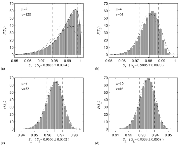
Figure 2: Histograms for the probability distribution $P(S_{L})$, numerically calculated from 1 million random states for the several subsystem dimensions $\mu$ and $\nu$ possible in a 256-dimensional Hilbert space. The exact means (vertical solid line) and standard deviations (vertical dashed line), along with Gaussian (dotted curve) and Airy function (dash-dotted curve) approximations to the distribution are also plotted. For $\mu=2$, the exact distribution (54) is plotted as the solid curve. Notice that for $\mu$ not too close to 2, the Gaussian approximation is sufficient and, as noted in the text, the linear entropy of a typical state, though close to maximal, is localized away from maximal.

Translating our results to the linear entropy, we have

$$\langle\!\langle S_{L}\rangle\!\rangle \equiv \langle S_{L}\rangle=\beta\frac{(\mu-1)(\nu-1)}{\mu\nu+1}\quad(\equiv a)\;,$$ (49)

$$\langle\!\langle S_{L}^{2}\rangle\!\rangle = \beta^{2}\langle\!\langle R^{2}\rangle\!\rangle\qquad\qquad\quad(\equiv b)\;,$$ (50)

$$\langle\!\langle S_{L}^{3}\rangle\!\rangle = -\beta^{3}\langle\!\langle R^{3}\rangle\!\rangle\;\quad\qquad\quad(\equiv c)\;.$$ (51)

These can be used in an approximation to the cumulant generating function and, hence, to the probability distribution itself:

$$P(S_{L})dS_{L} \approx \frac{1}{2\pi}\int_{-\infty}^{\infty}d\omega\,\exp\left[-iS_{L}\omega+ai\omega+b(i\omega)^{2}/2!+c(i\omega)^{3}/3!\right]dS_{L}$$ (52)

$$= |2/c|^{1/3}\exp\left[\frac{b^{3}}{3c^{2}}+\frac{b(S_{L}-a)}{c}\right]\mathrm{Ai}\left[(2/c)^{1/3}\left(S_{L}-a+\frac{b^{2}}{2c}\right)\right]dS_{L}\;.$$

When the overall dimension $\mu\nu$ is large, the standard deviation of the linear entropy is given approximately by

$$\langle\!\langle S_{L}^{2}\rangle\!\rangle^{1/2}\approx{\mu+1\over\mu\nu+1}\sqrt{{2\over\mu^{2}-1}}\left(1-{5\over 2\mu\nu}-{1\over 2\nu^{2}}\right)\;.$$ (53)

Comparing this with the average linear entropy shows that the bipartite entanglement of a typical pure state, though close to maximal, is nonetheless localized away from maximal as long as $\langle\!\langle S_{L}^{2}\rangle\!\rangle^{1/2}$ is somewhat smaller than $(\mu+1)/(\mu\nu+1)$, i.e., as long as $\mu$ is somewhat larger than 2.

In Fig. 2 we display numerical calculations of $P(S_{L})$ for the several ways of dividing a 256-dimensional Hilbert space into two subsystems. These numerical calculations used 1 million random states. We also plot the means (vertical solid line), standard deviations (vertical dashed line), the Airy function approximation (52) (dash-dotted curve), and the Gaussian approximation (dotted curve). For the special case $\mu=2$, the exact probability distribution is drawn (solid curve):

$$P(S_{L})\,dS_{L}=\frac{2\Gamma(\nu+1/2)}{\sqrt{\pi}\,\Gamma(\nu-1)}\sqrt{1-S_{L}}{S_{L}}^{\!\nu-2}dS_{L}\qquad(\mu=2)\;.$$ (54)

Note that the distributions are highly localized and that for $\mu$ somewhat larger than 2 in a high-dimensional overall space, the Gaussian approximation is sufficient.

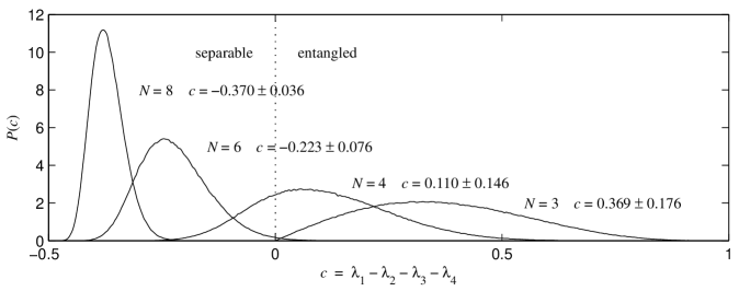
Figure 3: Pairwise mixed-state entanglement in random multi-qubit pure states with a total of 3, 4, 6, and 8 qubits. The plots show the probability distribution of the quantity $c(\hat{\rho})=\lambda_{1}-\lambda_{2}-\lambda_{3}-\lambda_{4}$. The concurrence is $C(\hat{\rho})=\max\{0,c(\hat{\rho})\}$. The means and standard deviations of the distributions are also given. The approximate probability to encounter pairwise entanglement between a particular pair of qubits in states with 3, 4, 6, and 8 total qubits is 1, 0.76, 0.006 and 0, respectively. The distributions were numerically calculated using 1 million random states.

III.2 Pairwise mixed-state entanglement

A numerical study of pairwise (mixed-state) entanglement in multi-qubit systems has already been published kendon , making the results in this section somewhat redundant. Our choice for an entanglement measure is the concurrence wootters of a two-qubit density operator $\hat{\rho}$, given by

$$C(\hat{\rho})\equiv\max\{0,\lambda_{1}-\lambda_{2}-\lambda_{3}-\lambda_{4}\}$$ (55)

where $\lambda_{1}\geq\lambda_{2}\geq\lambda_{3}\geq\lambda_{4}$ are the square roots of the eigenvalues of $\hat{\rho}(\hat{\sigma}_{y}\otimes\hat{\sigma}_{y})\hat{\rho}^{*}(\hat{\sigma}_{y}\otimes\hat{\sigma}_{y})$. The complex conjugation is taken in the standard qubit basis. The concurrence takes values in the range $[0,1]$, with a pair of qubits being entangled if and only if $C(\hat{\rho})>0$.

The concurrence provides an explicit formula for the entanglement of formation

$$E_{f}(\hat{\rho})\equiv\inf\sum_{j}p_{j}S(\psi_{j})\;,$$ (56)

where the infimum is taken over all pure-state decompositions $\hat{\rho}=\sum_{j}p_{j}|\psi_{j}\rangle\langle\psi_{j}|$, and $S(\psi_{j})$ is the subsystem von Neumann entropy of the bipartite pure state $\psi_{j}$ . In the case of two qubits,

$$E_{f}(\hat{\rho})={\cal E}\big{(}C(\hat{\rho})\big{)}\;,$$ (57)

where ${\cal E}$ is defined in terms of the binary entropy function $h(x)=-x\log x-(1-x)\log(1-x)$ by

$${\cal E}(C)\equiv h\!\left(\frac{1+\sqrt{1-C^{2}}}{2}\right)\;.$$ (58)

The function ${\cal E}(C)$ is monotonically increasing for $0\leq C\leq 1$, and hence the concurrence is a good measure of entanglement in its own right.

To apply the concurrence as a measure of pairwise entanglement in $N$-qubit pure states, we first trace out $N-2$ of the qubits and then use the above formulae on the resulting two-qubit density operator. In Fig. 3 we have plotted the probability distribution for the quantity

$$c(\hat{\rho})\equiv\lambda_{1}-\lambda_{2}-\lambda_{3}-\lambda_{4}\quad(-1/2\leq c\leq 1)\;,$$ (59)

when the $N$-qubit pure states are sampled from the Haar distribution for $N=3$, 4, 6, and 8. Notice that the probability of finding pairwise entanglement between any pair of qubits decreases rapidly as $N$ increases. In contrast, the preceding subsection shows that as $N$ increases, the bipartite entanglement of a typical state is close to maximal no matter how the overall system is sliced into two parts. Taken together, these results mean that the entanglement in a typical state of many qubits is mainly multipartite entanglement shared among many of the qubits, rather than pairwise entanglement.

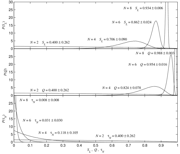
Figure 4: Multipartite entanglement in random multi-qubit pure states with a total of 2, 4, 6, and 8 qubits. The probability distributions are for the multipartite entanglement measures $Q$ and $\tau_{N}$. For comparison, the distributions for the subsystem linear entropy $S_{L}$ are also plotted in the case of equal subsystem dimensions ($\mu=\nu=\sqrt{D}$). The analytic values of the means and standard deviations are also shown. The distributions are based on numerical calculations using 1 million random states.

III.3 Multipartite entanglement

We now investigate two proposals for a measure of multipartite entanglement, the measure $Q$ of Meyer and Wallach meyer and the $n$-tangle of Wong and Christensen wong . In general, as the number of subsystems increases, an exponential number of independent measures is needed to quantify fully the amount entanglement in the multipartite system. Consequently, neither of the following entanglement measures can be thought of as unique. Different measures capture different aspects of multipartite entanglement.

The Meyer-Wallach measure, $Q(\psi)$, which can only be applied to multi-qubit pure states, is defined as follows. For each $\alpha=1,\dots,N$ and $b\in\{0,1\}$, we define the linear map $\imath_{\alpha}(b):(\mathbb{C}^{2})^{\otimes N}\rightarrow(\mathbb{C}^{2})^{\otimes N-1}$ through its action on the product basis,

$$\imath_{\alpha}(b)|x_{1}\rangle\otimes\dots\otimes|x_{N}\rangle=\delta_{bx_{\alpha}}|x_{1}\rangle\otimes\dots\otimes|x_{\alpha-1}\rangle\otimes|x_{\alpha+1}\rangle\otimes\dots\otimes|x_{N}\rangle\;.$$ (60)

Next let

$$D(\psi,\phi)=\sum_{i<j}|\psi_{i}\phi_{j}-\psi_{j}\phi_{i}|^{2}\;,$$ (61)

be the square of the wedge product of two vectors $|\psi\rangle$ and $|\phi\rangle$, where the $\psi_{j}$ are the coefficients of the state $|\psi\rangle$ in the product basis,

$$|\psi\rangle=\sum_{j=1}^{2^{m}}\psi_{j}|x_{1}\rangle\otimes\dots\otimes|x_{m}\rangle\;,\qquad j=x_{1}\ldots x_{m}\!\cdot\!0=\sum_{l=1}^{m}x_{l}2^{m-l}\;.$$ (62)

The Meyer-Wallach entanglement measure is then

$$Q(\psi)\equiv\frac{4}{N}\sum_{\alpha=1}^{N}D\big{(}\imath_{\alpha}(0)\psi,\imath_{\alpha}(1)\psi\big{)}\;.$$ (63)

Meyer and Wallach have shown that $Q$ is invariant under local unitary transformations and that $0\leq Q\leq 1$, with $Q(\psi)=0$ if and only if $|\psi\rangle$ is a product state. It was recently shown by Brennen brennen that $Q$ is simply the average subsystem linear entropy of the constituent qubits:

$$Q(\psi)=2\left(1-\frac{1}{N}\sum_{k=1}^{N}\,\text{tr}\,\hat{\rho}_{k}^{2}\right).$$ (64)

Here $\hat{\rho}_{k}$ is the density operator for the $k$-th qubit after tracing out the rest. Hence we should expect this measure to agree qualitatively with the subsystem entropies.

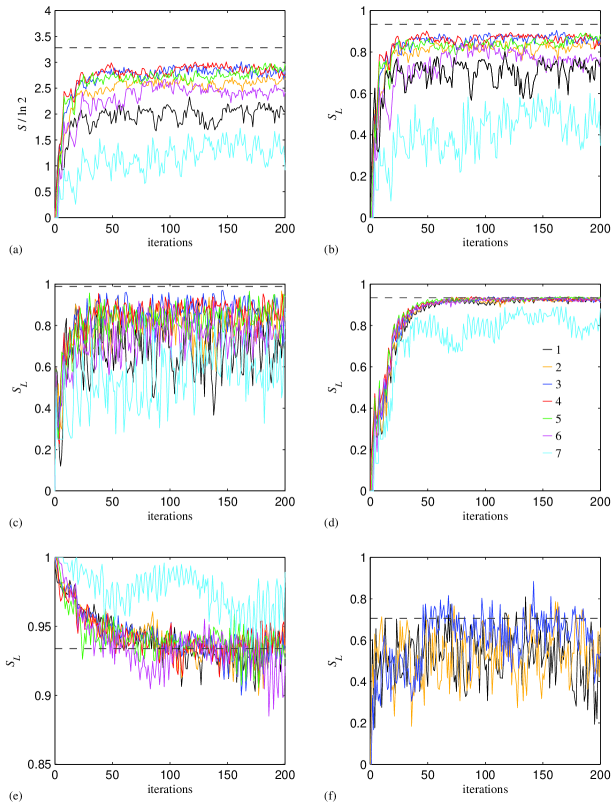
Figure 5: Dynamical behavior of the subsystem entropy. (a) and (b) plot the von Neumann entropy and the linear entropy, respectively, when $N=8$, the partition divides the four rightmost qubits from the four leftmost, and the initial state is $|00000000\rangle$. (c) is the same as (b), except that the partition divides the single rightmost qubit from the others. (d) and (e) are also the same as (b), but with initial state $|00100111\rangle$ in (d) and maximally entangled initial state (70) in (e). (f) shows the case of $N=4$ qubits, a partition that separates the two leftmost qubits from the two rightmost, and an initial state $|0000\rangle$. The different quantum baker’s maps are colored according to the key in (d). The dashed lines show the average entanglement predicted for random states.

Using, for example, the Hurwitz parametrization hurwitz ; pozniak of a random unit vector in $\mathbb{C}^{D}$, where the dimension $D=2^{N}$, one can calculate the mean and variance of $Q$ for random states:

$$\langle Q\rangle=\frac{D-2}{D+1}\;,$$ (65)

$$\langle\!\langle Q^{2}\rangle\!\rangle=\langle Q^{2}\rangle-\langle Q\rangle^{2}=\frac{6(D-4)}{(D+3)(D+2)(D+1)N}+\frac{18D}{(D+3)(D+2)(D+1)^{2}}\;.$$ (66)

The mean was also calculated independently in weinstein , and given the relationship (64), it can be easily checked using Lubkin’s formula for the average purity (32). For large $N$, the mean and standard deviation are given approximately by $\langle Q\rangle\approx 1-3/D$ and $\langle\!\langle Q^{2}\rangle\!\rangle^{1/2}\approx(1/D)\sqrt{6/N}$, indicating that the Meyer-Wallach entanglement of a typical state is very nearly maximal, but suggesting that this entanglement is weakly localized just below maximal.

In the case of two qubits, the square of the concurrence is often referred to as the tangle. A generalization of the tangle to three qubits was defined by Coffman et al. coffman . Wong and Christensen proposed another generalization valid for an arbitrary even number of qubits. For pure states of $N$ (even) qubits, it is defined as

$$\tau_{N}^{\phantom{2}}(\psi)\equiv|\langle\psi|\sigma_{y}^{\otimes N}|\psi^{*}\rangle|^{2}\qquad(N\textrm{ even})\;.$$ (67)

Wong and Christensen were able to show that $\tau_{N}$ is an entanglement monotone and also to generalize its definition to mixed states. From the above definition, it is easy to see that $0\leq\tau_{N}^{\phantom{2}}\leq 1$. A cat state, $(|0\rangle^{\otimes N}+|1\rangle^{\otimes N})/\sqrt{2}$, has maximal entanglement by this measure.

One can calculate the mean and variance of $\tau_{N}$ for random states:

$$\langle\tau_{N}^{\phantom{2}}\rangle=\frac{2}{D+1}\;,$$ (68)

$$\langle\!\langle\tau_{N}^{2}\rangle\!\rangle=\langle\tau_{N}^{2}\rangle-\langle\tau_{N}^{\phantom{2}}\rangle^{2}=\frac{4(D-1)}{(D+3)(D+1)^{2}}\;.$$ (69)

For large $N$, both the mean and the standard deviation of $\tau_{N}$ are given approximately by $2/D$, indicating that a typical state does not have whatever sort of multipartite entanglement is characterized by $\tau_{N}$.

In Fig. 4 we plot the probability distributions of $Q$ and $\tau_{N}$ after sampling 1 million random multi-qubit pure states with a total of 2, 4, 6, and 8 qubits. Also plotted, for comparison, are the corresponding distributions for the subsystem linear entropy $S_{L}$, with the two subsystem dimensions chosen to be equal. When $N=2$, the three different measures are equivalent, each having the distribution $P(E)\,dE=(3/2)\sqrt{1-E}\,dE$ ($E=S_{L},Q,\tau_{N}$). Notice, however, that the behaviors of the two multipartite measures diverge dramatically as we increase the total number of qubits. According to the Meyer-Wallach measure, multipartite entanglement increases as we increase the number of qubits. This agrees with the bipartite measure $S_{L}$, the only difference being that the Meyer-Wallach entanglement of a typical state is closer to maximal than the linear entropy as $N$ gets large. In contrast, the $n$-tangle of a typical state decreases as $N$ increases. As noted above, $\tau_{N}$ seems to describe some sort of multipartite entanglement that becomes rare as the number of qubits increases.

IV Entanglement production in the quantum baker’s maps

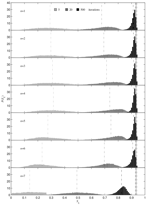
Figure 6: Distributions for the subsystem linear entropy, relative to a partition that divides the four least significant qubits from the four most significant, after 5, 20, and 500 iterations of the quantum baker’s maps starting with a uniform distribution of $16\,000$ product states (delta function centered at zero). A total of $N=8$ qubits is used. The dashed-dotted lines are the means of the distributions, and the mean and standard deviation for random states are the solid and dashed lines, respectively.

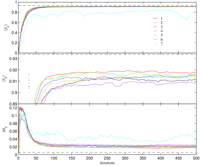
Figure 7: Evolution of the means and standard deviations for the subsystem linear entropy under the same conditions as in Fig. 6. The dashed lines are the mean and standard deviation for random states. The middle, magnified plot displays the ranking of the baker’s maps in terms of entangling power, i.e., 4,5,3,2,1,6,7. Error bars ($2\Delta S_{L}/\sqrt{16\,000}$) are included in the middle plot to indicate the expected sampling error for the means at saturation; these error bars show that the rankings in terms of entangling power are real, not statistical artifacts.

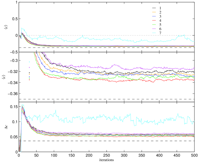
Figure 8: Evolution of the means and standard deviations for the quantity $c$ of Eq. (59), where all but the single leftmost and rightmost qubits are traced out. The concurrence for the remaining two qubits is $C=\max\{0,c\}$. The averages are taken with respect to $16\,000$ uniformly distributed initial product states for $N=8$ qubits. The dashed lines are the numerically calculated mean and standard deviation for random states. Error bars ($2\Delta c/\sqrt{16\,000}$) are included in the middle plot to indicate the expected sampling error for the means at saturation.

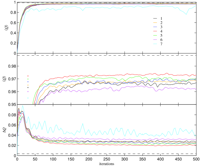
Figure 9: Evolution of the means and standard deviations for the Meyer-Wallach multipartite entanglement measure $Q$. The averages are taken with respect to $16\,000$ uniformly distributed initial product states for $N=8$ qubits. The dashed lines are the numerically calculated mean and standard deviation for random states. Error bars ($2\Delta Q/\sqrt{16\,000}$) are included in the middle plot to indicate the expected sampling error for the means at saturation.

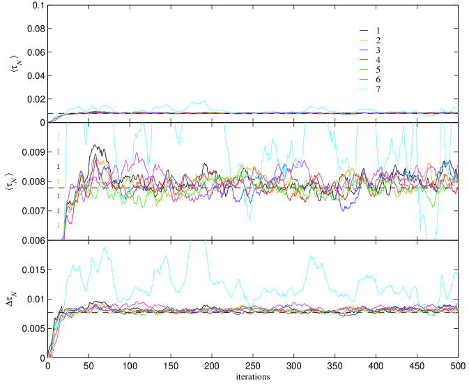
Figure 10: Evolution of the means and standard deviations for the Wong-Christensen tangle $\tau_{N}$. The averages are taken with respect to $16\,000$ uniformly distributed initial product states for $N=8$ qubits. The dashed lines are the numerically calculated mean and standard deviation for random states. Error bars ($2\Delta\tau_{N}/\sqrt{16\,000}$) are included in the middle plot to indicate the expected sampling error for the means at saturation.

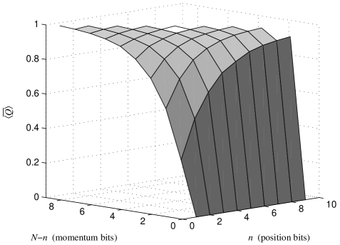
Figure 11: Saturation value $\overline{\langle Q\rangle}$ of the Meyer-Wallach entanglement measure for all quantum baker’s maps up to a total of $N=10$ qubits. This quantity is approximated by taking a time average over the $(512k)$-th iterates ($k=1,\dots,100$) and using $4\,000$ uniformly distributed initial product states.

We now report the results of a detailed numerical study of entanglement production for the quantum baker’s maps. All of the results reported in this section are for the 8-qubit baker’s maps (except for Fig. 5(f), which displays results for $N=4$ qubits). In the figures, the maps for different values of $n$ are distinguished by a color coding given in Fig. 5(d). The extreme map $\hat{B}_{N,N}$ is not included in the plots because it does not produce any entanglement.

First consider the bipartite measures of entanglement. In Fig. 5 we plot the dynamical behavior of these measures for several interesting initial states. Figure 5(a) shows the behavior of the subsystem von Neumann entropy $S$ when $N=8$ and the bipartite division is between the four least significant qubits (rightmost) and the four most significant (leftmost); in terms of the phase-space description of the baker’s maps, we are considering entanglement between the fine and coarse position scales on phase space. The initial state in Fig. 5(a) is the product state $|00000000\rangle$. Note the ranking among the different quantum baker’s maps. The maps $\hat{B}_{8,4}$ (red) and $\hat{B}_{8,3}$ (dark blue) achieve saturation values closest to that for typical states (dashed line). The original Balazs-Voros-Saraceno quantization has $n=1$ (black). Figure 5(b) is the same as (a), except now the linear entropy $S_{L}$ is our entanglement measure (as it remains in the remaining parts of Fig. 5). The two different definitions of entropy show the same qualitative behavior. In Fig. 5(c), we again use linear entropy, but switch to a bipartite division that separates the single rightmost qubit from the rest. The different saturation levels attained by the different quantum baker’s maps, though less intelligible, are still discernible. If we return to our original partition and change the initial state to $|00100111\rangle$, however, the differences in the saturation levels disappear almost altogether, as is shown in Fig. 5(d). The quantum baker’s map with $n=7$ stands out in all cases, saturating at a value well below the other maps; we should recall that the map $\hat{B}_{8,7}$ is closest to the map $\hat{B}_{8,8}$, which does not entangle at all. In Fig. 5(e), again using the original partition, we start in the entangled state

$${1\over 4}\sum_{x_{1},x_{2},x_{3},x_{4}}|x_{1}x_{2}x_{3}x_{4}x_{1}x_{2}x_{3}x_{4}\rangle\;,$$ (70)

which is maximally entangled with respect to the original partition. In this case the maximal initial level of entanglement is destroyed by the quantum baker’s maps. Figure 5(f) shows the case with $N=4$ qubits, a partition separating the two leftmost qubits from the two rightmost, and an initial state of $|0000\rangle$.

In view of the variety of behaviors exhibited by subtle differences in the initial states [compare Fig. 5(b) to 5(d)], if we are to study the intrinsic entangling properties of the quantum baker’s maps and not properties conditioned on a particular initial state, we need an approach that treats all initial states of a certain type on the same footing. Such neutrality can be achieved by taking an average over, for example, the set of all product states. This approach was used to define the entangling power zanardi of a unitary operator, and we adhere to it for the remainder of this section.

Consider starting with a uniform distribution of product pure states, each member being a tensor product of $N=8$ random single-qubit states. We now “bake” entanglement with the seven quantum baker’s maps. The remaining figures plot the amount of baked entanglement as quantified by the several entanglement measures discussed in Sec. III.

Figure 6 plots the distributions of the subsystem linear entropy, relative to a partition that divides the four least significant qubits from the four most significant, after 5, 20, and 500 iterations of the quantum baker’s maps. All the distributions start in a delta function centered at zero entanglement, but quickly spread while advancing toward the value predicted for typical states. The mean and standard deviation for random states are the solid and dashed lines, respectively. At 500 iterations, well after saturation ($\sim 100$), the mean entanglement for our quantum-baked states (dash-dotted lines) fall short of the value predicted for random states. Notice that the variances are also still quite large. For clarity, the means and standard deviations are plotted separately in Fig. 7. The ranking of the different quantum baker’s maps in terms of entangling power—4,5,3,2,1,6,7—is now only apparent after magnification at the saturation level (middle plot). It was found that this ranking is preserved when the partition is changed. If the total number of qubits is varied, similar behavior also results, and we conclude that the quantum baker’s maps are, in general, good generators of bipartite entanglement, with the highest levels produced when $n$ is roughly midway between $N$ and $1$. A total of $16\,000$ initial states were used in this simulation. The same number is used for those that follow.

We next consider the pairwise entanglement as given by the concurrence, or more specifically, by the quantity $c(\hat{\rho})$ of Eq. (59). We only display results for the case where all but the single leftmost and rightmost qubits are traced out. The other cases are similar. Again, starting in a uniform distribution of $16\,000$ product states (delta function centered at $c=0$), we bake entanglement into our states. In this case, however, the pairwise entanglement is not maintained. After a short rise, $c(\hat{\rho})$ quickly falls to negative values, retreating toward the mean numerically calculated for random states, as shown in Fig. 8. Not surprisingly, the quantum baker’s maps respect the rarity of pairwise entanglement in multi-qubit states. The ranking among the different quantum baker’s maps is also preserved.

In Figs. 9 and 10, we plot the corresponding evolutions for multipartite entanglement measures, the Meyer-Wallach measure $Q$ and Wong-Christensen $\tau_{N}$. The means and standard deviations of $Q$ behave similarly to the bipartite measures of entanglement. The ranking among the different quantum baker’s maps is again preserved. This is not surprising given the relationship (64). In the case of $\tau_{N}$, however, it is difficult to discern any useful information, presumably because this measure only describes entanglement of a very special type, e.g., that in $N$-qubit cat states.

V Discussion and Conclusion

The numerical calculations of the previous section show that the quantum baker’s maps are, in general, good at creating multipartite entanglement amongst the qubits. It was found, however, that some quantum baker’s maps can, on average, entangle better than others, and that all quantum baker’s maps fall somewhat short of generating the levels of entanglement expected in random states. This might be related to the fact that spatial symmetries in the baker’s map allow deviations from the predictions of random matrix theory balazs . Such deviations are apparent in the statistics of the eigenvectors of $\hat{B}_{N,n}$ and might also taint the randomness of our quantum-baked states. In this light, an entanglement measure might, in fact, provide a reasonable test for the randomness of states produced by a quantum map.

In our case, entanglement amongst the qubits relates directly to correlations between the coarse and fine scales of classical phase space. Although we have only considered entanglement in position, the Fourier transform provides a means to investigate entanglement in momentum, and the partial Fourier transform (10) might be used for all intermediate possibilities. These qubit bases, while naturally embedded in the construction of the quantum baker’s maps, might also be applied to other maps of the unit square and, hence, to entanglement production in general for quantized mappings of the torus.

We should expect high levels of entanglement creation in quantum maps that are chaotic in their classical limit. Such maps have a dynamical behavior that produces correlations between the coarse and fine scales of phase space. This behavior is described classically in the form of symbolic dynamics. Investigations into entanglement production, using the above product bases, allow us to characterize the quantum version of such correlations. To develop a complete picture, however, the entangling properties of regular systems must first be addressed. The possibility of nonentangling quantum maps, such as $\hat{B}_{N,N}$, which produce stochasticity in their classical limit, must also be addressed.

We can apply our results to a preliminary investigation of the relation between entanglement production and the classical limit. As remarked previously, sequences of quantum baker’s maps for which the number of momentum bits, $N-n$, is held constant do not approach the classical baker’s map in the limit $N\rightarrow\infty$, but instead give rise to stochastic variants. To relate this behavior to entanglement production, consider the time average of the Meyer-Wallach entanglement measure $Q$, say,

$$\overline{\langle Q\rangle}\equiv\lim_{m\rightarrow\infty}{1\over m}\sum_{k=1}^{m}\langle Q\rangle_{k}$$ (71)

where, as before, the average $\langle\>\cdot\>\rangle$ is taken over a uniform distribution of initial product states. This quantity provides the long time saturation value of $Q$ and is plotted for all quantum baker’s maps up to total of $N=10$ qubits in Fig. 11. Note that although one observes a drop in the levels of entanglement for a small number of position bits, $n$, there is no apparent connection between the level of $\overline{\langle Q\rangle}$ and the advent of spurious stochastic limits when the number of momentum bits, $N-n$, remains constant as $N$ increases. One might have expected the saturation value to be suppressed in such limits, but this appears not to be the case. We tentatively conclude that entanglement production in the qubit bases is unrelated to the creation of a stochasticity in the classical limit. A similar picture emerges when the subsystem entropy is used as the entanglement measure.

In conclusion, we have found that the quantum baker’s maps are, in general, good at generating multipartite entanglement amongst qubits. Given the relation between our qubit bases and classical phase space, this behavior should be expected to arise whenever such a quantum map is chaotic in its classical limit.

- (1) Lichtenberg A J and Lieberman M A 1992 Regular and Chaotic Dynamics (New York: Springer)
- (2) Balazs N L and Voros A 1989 Ann. Phys. 190 1
- (3) Saraceno M 1990 Ann. Phys. 199 37
- (4) Hannay J H, Keating J P and Ozorio de Almeida A M 1994 Nonlinearity 7 1327
- (5) Rubin R and Salwen N 1998 Ann. Phys. 269 159
- (6) Lesniewski A, Rubin R and Salwen N 1998 J. Math. Phys. 39 1835
- (7) Schack R 1998 Phys. Rev. A 57 1634
- (8) Brun T A and Schack R 1999 Phys. Rev. A 59 2649
- (9) Pakoński P, Ostruszka A and Życzkowski K 1999 Nonlinearity 12 269
- (10) Schack R and Caves C M 2000 Applicable Algebra in Engineering, Communication and Computing 10 305
- (11) Soklakov A N and Schack R 2000 Phys. Rev. E 61 5108
- (12) Tracy M M and Scott A J 2002 J. Phys. A 35 8341
- (13) Sakagami M, Kubotani H and Okamura T 1996 Prog. Theor. Phys. 95 703
- (14) Tanaka A 1996 J. Phys. A 29 5475
- (15) Furuya K, Nemes M C and Pellegrino G Q 1998 Phys. Rev. Lett. 80 5524
- (16) Angelo R M, Furuya K, Nemes M C and Pellegrino G Q 1999 Phys. Rev. E 60 5407
- (17) Miller P A and Sarkar S 1999 Phys. Rev. E 60 1542
- (18) Lakshminarayan A 2001 Phys. Rev. E 64 036207
- (19) Bandyopadhyay J N and Lakshminarayan A 2002 Phys. Rev. Lett. 89 060402
- (20) Tanaka A, Fujisaki H and Miyadera T 2002 Phys. Rev. E 66 045201
- (21) Fujisaki H, Miyadera T and Tanaka A 2003 Phys. Rev. E 67 066201
- (22) Lahiri A e-print quant-ph/0302029
- (23) Lakshminarayan A and Subrahmanyam V 2003 Phys. Rev. A 67 052304
- (24) Bettelli S and Shepelyansky D L 2003 Phys. Rev. A 67 054303
- (25) Nielsen M A and Chuang I L 2000 Quantum Computation and Quantum Information (Cambridge: Cambridge University Press)
- (26) Haake F 1991 Quantum Signatures of Chaos (Berlin: Springer)
- (27) Guhr T, Müller-Groeling A and Weidenmüller H A 1998 Phys. Rep. 299 189
- (28) Brody T A, Flores J, French J B, Mello P A, Pandey A and Wong S S M 1981 Rev. Mod. Phys. 53 385
- (29) Horodecki M 2001 Quantum Inf. Comput. 1 3
- (30) Wootters W K 2001 Quantum Inf. Comput. 1 27
- (31) Horodecki P and Horodecki R 2001 Quantum Inf. Comput. 1 45
- (32) Nielsen M A and Vidal G 2001 Quantum Inf. Comput. 1 76
- (33) Bennett C H, DiVincenzo D P, Smolin J A and Wootters W K 1996 Phys. Rev. A 54 3824
- (34) Popescu S and Rohrlich D 1997 Phys. Rev. A 56 3319
- (35) Życzkowski K and Sommers H-J 2001 J. Phys. A 34 7111
- (36) Bennett C H, Brassard G, Popescu S, Schumacher B, Smolin J A and Wootters W K 1996 Phys. Rev. Lett. 76 722
- (37) Vedral V, Plenio M B, Rippin M A and Knight P L 1997 Phys. Rev. Lett. 78 2275
- (38) Vedral V and Plenio M B 1998 Phys. Rev. A 57 1619
- (39) Hill S and Wootters W K 1997 Phys. Rev. Lett. 78 5022
- (40) Wootters W K 1998 Phys. Rev. Lett. 80 2245
- (41) Lloyd S and Pagels H 1988 Ann. Phys. (N.Y.) 188 186
- (42) Page D N 1993 Phys. Rev. Lett. 71 1291
- (43) Foong S K and Kanno S 1994 Phys. Rev. Lett. 72 1148
- (44) Sánchez-Ruiz J 1995 Phys. Rev. E 52 5653
- (45) Sen S 1996 Phys. Rev. Lett. 77 1
- (46) Gemmer J, Otte A and Mahler G 2001 Phys. Rev. Lett. 86 1927
- (47) Malacarne L C, Mendes R S and Lenzi E K 2002 Phys. Rev. E 65 046131
- (48) Lubkin E 1978 J. Math. Phys. 19 1028
- (49) Gradshteyn I S and Ryzhik I M 1980 Table of Integrals, Series and Products (New York: Academic)
- (50) Kendon V M, Nemoto K and Munro W J 2002 J. Mod. Optics 49 1709
- (51) Meyer D A and Wallach N R 2002 J. Math. Phys. 43 4273
- (52) Wong A and Christensen N 2001 Phys. Rev. A 63 044301
- (53) Brennen G K e-print quant-ph/0305094
- (54) Hurwitz A 1897 Nachr. Ges. Wiss. Gött. Math.-Phys. Kl 71
- (55) Poźniak M, Życzkowski K and Kuś M 1998 J. Phys. A 31 1059
- (56) Emerson J, Weinstein Y S, Saraceno M, Lloyd S and Cory D G preprint
- (57) Coffman V, Kundu J and Wootters W K 2000 Phys. Rev. A 61 052306
- (58) Zanardi P, Zalka C and Faoro L 2000 Phys. Rev. A 62 030301