Output state in multiple entanglement swapping

Abstract

The technique of quantum repeaters is a promising candidate for sending quantum states over long distances through a lossy channel. The usual discussions of this technique deals with only a finite dimensional Hilbert space. However the qubits with which one implements this procedure will “ride” on continuous degrees of freedom of the carrier particles. Here we analyze the action of quantum repeaters using a model based on pulsed parametric down conversion entanglement swapping. Our model contains some basic traits of a real experiment. We show that the state created, after the use of any number of parametric down converters in a series of entanglement swappings, is always an entangled (actually distillable) state, although of a different form than the one that is usually assumed. Furthermore, the output state always violates a Bell inequality.

I Introduction

Entanglement cannot be created by local operations and classical communication between the parties. However it was shown in Ref. ZZHE (see also SougatoSwap ) that there exists an operational scheme, such that particles can get entangled without ever having interacted in the past. One of the intruiging things about this phenomenon, which has been called entanglement swapping, is that it shows that one cannot always tell whether particles are entangled by looking at their “common history”. Or the concept of “common history” must be suitably enlarged. Note that entanglement swapping process is a specific case of quantum teleportation tele . The first experimental realization of entanglement swapping was reported in Pan . The experiment was a direct realization of the experimental procedure given in ZZHE , and modified in ZukowskiSwapProc .

As a simple illustration of this phenomenon, consider the situation in which Alice and Bob, share the singlet $\left|\psi^{-}\right\rangle=\frac{1}{\sqrt{2}}(\left|01\right\rangle-\left|10\right\rangle)$, and Alice shares another singlet with Claire. Alice now makes a projection measurement on her parts of the two singlets in the Bell basis, given by the states

$$\begin{array}[]{lcl}\left|\phi^{\pm}\right\rangle=\frac{1}{\sqrt{2}}(\left|00\right\rangle\pm\left|11\right\rangle),\\ \left|\psi^{\pm}\right\rangle=\frac{1}{\sqrt{2}}(\left|01\right\rangle\pm\left|10\right\rangle).\end{array}$$ (1)

It is easy to check that if Alice now communicates (over a classical channel) the result of her measurement to Bob and Claire, they will know that they share one of the Bell states given by eq. (1). Note that in principle the particles of Bob and Claire may not have interacted in the past, although they share entanglement after Alice’s classical communication to them.

Apart from this fundamental perspective, entanglement swapping is also important in quantum communication applications. When sending a quantum state over a noisy channel, the probability that it reaches the recipient, decreases with the length of the channel. However, the detectors at the recipient’s end are usually (rather invariably) noisy, and this noise is independent of the length of the channel. Thus after a critical length, the signal is useless. To circumvent this problem, a proposal was provided Briegel that places a number of nodes in between the sender and the recipient of the signal. Entangled states are first shared in these shorter segments (i.e. between all successive nodes) and thereafter distilled huge to obtain highly entangled states between all successive nodes (Fig. 1).

Figure 1: Quantum repeaters: A chain of maximally entangled states obtained after distilations, are shared between the sender, the nodes at $A$, $B$, $\ldots$, $N$ and the recipient. Bell measurements are performed at the nodes. This results in an entangled state shared by the sender and the reciepent.

Finally entanglement swapping is carried out at all nodes to obtain highly entangled states between the sender and the recipient (henceforth called Alice and Bob respectively). It was shown Briegel that this procedure, called quantum repeaters, would lead to highly entangled states between the ends of a noisy channel of arbitrary length, with only a polynomial increase in time and logarithmic increase in local resources.

Usual discussions on quantum repeaters deal with only a finite dimensional Hilbert space. But the qubits with which one implements this procedure will “ride” on continuous degrees of freedom of the carrier particles. In this paper, we address the problem of implementation of this procedure of quantum repeaters, for the entangled states prepared between successive nodes by spontaneous pulsed parametric down conversion ZZHE ; ZukowskiSwapProc . The discussion of the process will follow the ones of Refs. ZZHE ; ZukowskiSwapProc . The experimental realization of entanglement swapping fully confirmed the validity of this description Pan . Actually in the experiment, polarization entanglement was utilized. But it is elementary to show the equivalence of such experiment with ones involving path entanglement, which will be our model here (see Ref. ZHWZ ). In this paper, we assume that the noise in the channel from a parametric down conversion crystal to the nearest nodes is negligible. Entanglement swapping is carried out at all the nodes.

The description of entanglement swapping that we consider in this paper, is still a toy model. Nevertheless it contains some basic traits of a possible real experiment. We show that the final state prepared between Alice and Bob is a so-called maximally correlated state, which is always entangled (actually distillable) and always violates a Bell inequality. For a wide range of pulses and filters, including Gaussian pulses and filters, the output two qubit state created between Alice and Bob turns out to be a mixture of two Bell states,

$$\frac{1+V}{2}\left|\phi^{+}\right\rangle\left\langle\phi^{+}\right|+\frac{1-V}{2}\left|\phi^{-}\right\rangle\left\langle\phi^{-}\right|,$$

where $\left|\phi^{\pm}\right\rangle$ are given by eq. (1) and where $0\leq V\leq 1$.

II Double entanglement swapping

Consider the case of three parametric down conversion crystals producing three entangled states between the sender (Alice) and $A_{1}$, $A_{2}$ and $B_{1}$, and $B_{2}$ and the recipient (Bob) (see Fig. 2)footnote_noi .

Figure 2: Quantum repeaters: A chain of three states.

Entanglement swapping will be carried out at $A_{1}A_{2}$ and $B_{1}B_{2}$. In Fig. 3, we give a schematic description of entanglement swapping in an array of three type I spontaneous parametric down conversions (PDC) ZZHE ; ZukowskiSwapProc . Note that frequency filters are in front of every beamsplitter, in the “internal” part of the device. They are necessary to make the photons emerging independently from two different sources, indistinguishable by the detectors behind the beamsplitters (for the physical reasons for this, see ZZHE ; ZukowskiSwapProc ).

Figure 3: Entanglement swapping in a chain of three parametric down converters. The boxes denoted as PDC-I, PDC-II, and PDC-III symbolizes the full parametric down conversion device, including the pump laser, crystal, a set of apertures that select suitable output directions, as well as suitably oriented mirrors that direct the radiation into the interferometers shown in the figure. The radiation at the detectors $i_{1},\ldots,i_{4}$ and $i_{1}^{{}^{\prime}},\ldots,i_{4}^{{}^{\prime}}$ is observed by detectors. The interferometers are built out of mirrors $M$ and 50-50 beamsplitters (BS). We need to put suitable frequency filters in front of all BS leading to the internal outputs $i_{(.)}$ and $i_{(.)}^{{}^{\prime}}$. The symbols $\phi$ and $\phi^{{}^{\prime}}$ denote the local phase shifters. For simplicity, we shall study the case when only four internal detectors (the “i”s) fire (those marked with asterix). Due to the specific properties of downconversion ZZHE ; ZukowskiSwapProc , no filters are needed in the output beams of the device, $a$ and $f$.

We make the simplifying assumptions that the optical lengths of all source-detector paths are equal and that phase shifters work in the range of the order of the wavelength (i.e. between 0 and $2\pi$). This enables us to neglect all retardation effects.

The description of the two-photon initial entangled state will depend on whether the corresponding PDC is an “external” or an “internal” one, in the series of PDCs. In any series of PDCs, there will be two external ones, while the rest will be called internal. For example, in the case of three PDCs, as described in Fig. 3, PDC-I and PDC-III are externals, while PDC-II is an internal one. If the “idler” photon emitted by the external PDCs in Fig. 3 (produced by a single pulse from a laser pump), manages to pass via the filters, the resulting two-photon state is given by (see Appendix)

$$\left|\psi_{ext}(x,y,x^{{}^{\prime}},y^{{}^{\prime}})\right\rangle=\int d\omega_{i}\int d\omega_{s}\int d\omega_{p}F(\omega_{p})\Delta(\omega_{p}-\omega_{i}-\omega_{s})f(\omega_{i})(a_{x}^{\dagger}(\omega_{i})a_{y}^{\dagger}(\omega_{s})+a_{x^{{}^{\prime}}}^{\dagger}(\omega_{i})a_{y^{{}^{\prime}}}^{\dagger}(\omega_{s}))\left|\Omega\right\rangle,$$ (2)

where $a_{x}^{\dagger}(\omega_{i})$ ($a_{y}^{\dagger}(\omega_{s})$) and $a_{x^{{}^{\prime}}}^{\dagger}(\omega_{i})$ ($a_{y^{{}^{\prime}}}^{\dagger}(\omega_{s})$) are the creation operators of photons of the idler (signal) of frequency $\omega_{i}$ ($\omega_{s}$) respectively in beams $x$ and $x^{{}^{\prime}}$ ($y$ and $y^{{}^{\prime}}$). The function $F$ represents the spectral content of the pump pulse of frequency $\omega_{p}$ and $f$ is the transmission function of the filters and is assumed to be centered at $\omega_{0}/2$, where in turn, $\omega_{0}$ is the central frequency of the laser pump pulse. The function $\Delta(\omega_{p}-\omega_{i}-\omega_{s})$ is due to the phase-matching condition of the PDC process. $\left|\Omega\right\rangle$ is the vacuum state. The state produced at PDC-I is $\left|\psi_{ext}(b,a,b^{{}^{\prime}},a^{{}^{\prime}})\right\rangle$ and that at PDC-III is $\left|\psi_{ext}(f,e,f^{{}^{\prime}},e^{{}^{\prime}})\right\rangle$. We assume, in all our considerations, the perfect case and so we will replace our $\Delta$ by the Dirac delta function. Here and henceforth, unless stated otherwise, we ignore normalization of states.

If the two photons produced by the internal PDC (PDC-II) in Fig. 3, manage to pass the filters, their state acquires the following form (see Appendix):

$$\left|\psi_{int}(d,c,d^{{}^{\prime}},c^{{}^{\prime}})\right\rangle=\int d\omega_{i}^{{}^{\prime}}\int d\omega^{{}^{\prime}}_{s}\int d\omega^{{}^{\prime}}_{p}F(\omega^{{}^{\prime}}_{p})\Delta(\omega^{{}^{\prime}}_{p}-\omega^{{}^{\prime}}_{i}-\omega^{{}^{\prime}}_{s})f(\omega^{{}^{\prime}}_{i})f(\omega^{{}^{\prime}}_{s})(a_{d}^{\dagger}(\omega_{i}^{{}^{\prime}})a_{c}^{\dagger}(\omega_{s}^{{}^{\prime}})+a_{d^{{}^{\prime}}}^{\dagger}(\omega_{i}^{{}^{\prime}})a_{c^{{}^{\prime}}}^{\dagger}(\omega_{s}^{{}^{\prime}}))\left|\Omega\right\rangle.$$ (3)

Note that there is an extra filter function in this case. This is a signature of the fact that both the photons from PDC-II are detected by the internal detectors and to reach there, they must pass the filters. In the general case of an arbitrary number (say, $n$) of PDCs in a series, there will be two entangled pairs described by eq. (2), while there will be $n-2$ “internal” entangled pairs described by eq. (3). Note here that previous works on entanglement swapping with two PDCs ZZHE ; ZukowskiSwapProc did not need to consider any “internal” entangled pairs.

In the case of entanglement swapping by $3$ PDCs (as shown in Fig. 3), our initial state, if all photons manage to pass the filters, is given by

$$\begin{array}[]{lcl}&&\left|\Psi\right\rangle=\\ &&\left|\psi_{ext}(f,e,f^{{}^{\prime}},e^{{}^{\prime}})\right\rangle\left|\psi_{int}(d,c,d^{{}^{\prime}},c^{{}^{\prime}})\right\rangle\left|\psi_{ext}(b,a,b^{{}^{\prime}},a^{{}^{\prime}})\right\rangle.\end{array}$$

Now suppose that the detector $i_{1}$ fires at time $t_{1}$, $i_{2}$ at time $t_{2}$, $i_{3}$ at time $t_{3}$, and $i_{4}$ at time $t_{4}$. Then the wave packet collapses into the state

$$\left|\Psi;t_{1},t_{2},t_{3},t_{4}\right\rangle=i_{1}(t_{1})i_{2}(t_{2})i_{3}(t_{3})i_{4}(t_{4})\left|\Psi\right\rangle$$ (4)

where, for example,

$$i_{1}(t_{1})=\int d\omega\exp\{-i\omega t_{1}\}a_{i_{1}}(\omega).$$

Note that the scalar product of $\int d\omega\exp\{i\omega t_{1}\}a_{i_{1}}^{\dagger}(\omega)$ with a single photon state

$$\int d\omega g(\omega)a^{\dagger}_{i_{1}}(\omega)\left|\Omega\right\rangle$$

gives the probability amplitude to detect this photons at time $t_{1}$. Let us assume that our 50-50 beamsplitters (BS) are the symmetric ones. That is, one has, e.g.

$$a_{i_{1}}^{\dagger}(\omega)=\frac{1}{\sqrt{2}}\left(a_{c^{{}^{\prime}}}^{\dagger}(\omega)+ia_{b^{{}^{\prime}}}^{\dagger}(\omega)\right).$$

Note that the creation operator of the reflected beam always enters the relation for $a_{i_{k}}^{\dagger}$ with an $i$ factor. As we consider here the idealized case, we substitute $\Delta$ by Dirac delta functions to obtain

$$\left|\Psi;t_{1},t_{2},t_{3},t_{4}\right\rangle=\int dtF^{*}(t)f(t-t_{4})f(t-t_{1})a_{f}^{\dagger}[g,t_{3}]a_{a}^{\dagger}[g,t_{2}]+\int dtF^{*}(t)f(t-t_{3})f(t-t_{2})a_{f^{{}^{\prime}}}^{\dagger}[g,t_{4}]a_{a^{{}^{\prime}}}^{\dagger}[g,t_{1}],$$ (5)

where we denote for example,

$$a_{f}^{\dagger}[g,t_{3}]=\int d\omega_{s}g(\omega_{s},t_{3})a_{f}^{\dagger}(\omega_{s})$$

with

$$g(\omega_{s},t_{3})=\int dt\exp\{i\omega_{s}t\}F^{*}(t)f(t-t_{3}).$$

After the photons in the state $\left|\Psi;t_{1},t_{2},t_{3},t_{4}\right\rangle$ pass through the phase shifters (as depicted in Fig. 3), the new state, $\left|\Psi;t_{1},t_{2},t_{3},t_{4},\phi,\phi^{{}^{\prime}}\right\rangle$, is obtained by replacing $a^{\dagger}_{a^{{}^{\prime}}}$ by $\exp\{i\phi\}a^{\dagger}_{a^{{}^{\prime}}}$ and $a^{\dagger}_{f}$ by $\exp\{i\phi^{{}^{\prime}}\}a^{\dagger}_{f}$. Let us assume now that the photons (after passing through phase shifters and 50-50 beam splitters (cf. Fig. 3)) are detected at $a_{+}$ and $f_{+}$ at times $t_{a}$ and $t_{f}$ respectively. Hence the amplitude of such a process is

$$\begin{array}[]{lcl}&&A_{a_{+},f_{+}}(t_{a},t_{f},t_{1},t_{2},t_{3},t_{4})=\\ &&\left\langle f_{+}(t_{f}),a_{+}(t_{a})\right|\left|\Psi;t_{1},t_{2},t_{3},t_{4},\phi,\phi^{{}^{\prime}}\right\rangle,\end{array}$$

where, for example,

$$\begin{array}[]{lcl}\left|f_{+}(t_{f}),a_{+}(t_{a})\right\rangle&=&\int d\omega\exp\{i\omega t_{f}\}a^{\dagger}_{f_{+}}(\omega)\\ &&\int d\omega^{{}^{\prime}}\exp\{i\omega^{{}^{\prime}}t_{a}\}a^{\dagger}_{a_{+}}(\omega^{{}^{\prime}})\left|\Omega\right\rangle.\end{array}$$

Writing it out explicitly, one obtains

$$A_{a_{+},f_{+}}=\exp\{i(\phi-\phi^{{}^{\prime}})\}T_{1}+T_{2},$$

where

$$\begin{array}[]{lcl}&&T_{1}=T(t_{a},t_{f},t_{1},t_{2},t_{3},t_{4})\\ &&\equiv\int dtdt^{{}^{\prime}}dt^{{}^{\prime\prime}}\int d\omega_{s}d\omega_{s}^{{}^{\prime\prime}}\exp\{i(\omega^{{}^{\prime\prime}}_{s}t+\omega_{s}t^{{}^{\prime}})\}\times\\ &&\exp\{-i(\omega^{{}^{\prime\prime}}_{s}t_{f}+\omega_{s}t_{a})\}F^{*}(t)F^{*}(t^{{}^{\prime}})F^{*}(t^{{}^{\prime\prime}})\times\\ &&f(t-t_{3})f(t^{{}^{\prime}}-t_{2})f(t^{{}^{\prime\prime}}-t_{4})f(t^{{}^{\prime\prime}}-t_{1})\end{array}$$ (6)

and

$$T_{2}=T(t_{a},t_{f},t_{2},t_{1},t_{4},t_{3}).$$

However, due to the finite time resolution of the detectors, the precise detection times are not known. Therefore the full probability, $P$, of the process is obtained after integration of the square of the amplitude over the detection times:

$$\begin{array}[]{lcl}&&P(a_{+},f_{+})=\int[|T_{1}|^{2}+|T_{2}|^{2}\\ &&+2\cos(\phi-\phi^{{}^{\prime}}+\phi_{0})|T_{1}T_{2}^{*}|]dt_{1}dt_{2}dt_{3}dt_{4}dt_{f}dt_{a}\end{array}$$ (7)

(where $\phi_{0}$ is a phase). We integrate here from $-\infty$ to $+\infty$, because the time resolution of detectors is usually by orders of magnitude bigger than the duration of the pumping pulse. We can now calculate the interferometric contrast, or the visibility

$$V_{3}=\frac{\max P-\min P}{\max P+\min P},$$

of the two particle interference process as observed by changing the values of the local phase shifts in the two external interferometers. (The index $3$ stands for the number of PDCs involved.) The resulting value is given by

$$V_{3}=\frac{2\int|T_{1}T_{2}^{*}|dt_{1}dt_{2}dt_{3}dt_{4}dt_{f}dt_{a}}{\int(|T_{1}|^{2}+|T_{2}|^{2})dt_{1}dt_{2}dt_{3}dt_{4}dt_{f}dt_{a}}.$$ (8)

We will now write down the explicit forms of the expressions in the numerator and denominator of $V_{3}$. We have

$$\begin{array}[]{lcl}F_{1234}&\equiv&\int|T_{1}T_{2}^{*}|dt_{1}dt_{2}dt_{3}dt_{4}dt_{f}dt_{a}\\ &=&\int dt_{1}dt_{2}dt_{3}dt_{4}|\int dtdt^{{}^{\prime}}dt^{{}^{\prime\prime}}d\overline{t^{{}^{\prime\prime}}}\times\\ &&|F(t)|^{2}|F(t^{{}^{\prime}})|^{2}F^{*}(t^{{}^{\prime\prime}})F(\overline{t^{{}^{\prime\prime}}})\times\\ &&f(t-t_{3})f^{*}(t-t_{4})f(t^{{}^{\prime}}-t_{2})f^{*}(t^{{}^{\prime}}-t_{1})\times\\ &&f(t^{{}^{\prime\prime}}-t_{4})f(t^{{}^{\prime\prime}}-t_{1})f^{*}(\overline{t^{{}^{\prime\prime}}}-t_{3})f^{*}(\overline{t^{{}^{\prime\prime}}}-t_{2})|.\end{array}$$ (9)

Throughout the paper, a “bar” will represent a new variable. This should not be confused with complex conjugation, which we denote here by a “^∗”.

A similar simplifying gives

$$\begin{array}[]{lcl}G_{1234}&\equiv&\int|T_{1}|^{2}dt_{1}dt_{2}dt_{3}dt_{4}dt_{f}dt_{a}\\ &=&\int dtdt^{{}^{\prime}}dt^{{}^{\prime\prime}}d\overline{t^{{}^{\prime\prime}}}\int dt_{1}dt_{2}dt_{3}dt_{4}\times\\ &&|F(t)|^{2}|F(t^{{}^{\prime}})|^{2}F^{*}(t^{{}^{\prime\prime}})F(\overline{t^{{}^{\prime\prime}}})\times\\ &&|f(t-t_{3})|^{2}|f(t^{{}^{\prime}}-t_{2})|^{2}f(t^{{}^{\prime\prime}}-t_{4})f(t^{{}^{\prime\prime}}-t_{1})\times\\ &&f^{*}(\overline{t^{{}^{\prime\prime}}}-t_{4})f^{*}(\overline{t^{{}^{\prime\prime}}}-t_{1}).\end{array}$$ (10)

Note that in $G_{1234}$, the indices are ordered. One can easily find that

$$\int|T_{2}|^{2}dt_{1}dt_{2}dt_{3}dt_{4}dt_{f}dt_{a}=G_{2143}.$$ (11)

Hence the visibility of the two particle interference that can be obtained due to the two-fold entanglement swapping (Fig. 3), is given by

$$\begin{array}[]{rcl}V_{3}=\frac{2{F_{1234}}}{G_{1234}+G_{2143}}.\end{array}$$ (12)

III Arbitrary number of swappings

Consider now a chain (i.e., arranged in a series) of any number, $n$, of PDCs (see Fig. 1). Let $a^{(1)}$ and $a^{{}^{\prime}(1)}$ denote the paths within the external interferometer into which one of the photons from the first PDC enters. The paths within the other external interferometer, into which enters the photon from the last PDcs will be denoted as $a^{(n)}$ and $a^{{}^{\prime}(n)}$. Let $\omega_{s}^{(1)}$ and $\omega_{s}^{(n)}$ be the corresponding frequencies of the photons. If all the photons manage through the frequency filters, the state is

$$\left|\psi^{(1)}\right\rangle\otimes\left(\otimes_{l=2}^{n-2}\left|\psi^{(l)}\right\rangle\right)\otimes\left|\psi^{(n)}\right\rangle$$ (13)

with the states $\left|\psi^{(1)}\right\rangle$ and $\left|\psi^{(n)}\right\rangle$ of the type characteristic for the external PDCs and $\left|\psi^{(l)}\right\rangle$ ($l=2,\ldots,n-2$) for the internal ones (compare eqs. (2) and (3)). Imagine now that again all internal detectors $i_{k}$, $k=1,2,\ldots,2n-2$ fire. The final state into which the state in eq. (13) collapses is of the following form:

$$\begin{array}[]{rcl}\left|\chi_{t}\right\rangle&=&\int d\omega^{(1)}_{s}d\omega^{(n)}_{s}(X_{t}(\omega^{(1)}_{s},\omega^{(n}_{s})a_{a^{(n)}}^{\dagger}(\omega^{(n)}_{s})a_{a^{{}^{\prime}(1)}}^{\dagger}(\omega^{(1)}_{s})\\ &+&Y_{t}(\omega^{(1)}_{s},\omega^{(n)}_{s})a_{a^{{}^{\prime}(n)}}^{\dagger}(\omega^{(n)}_{s})a_{a^{(1)}}^{\dagger}(\omega^{(1)}_{s}))\left|\Omega\right\rangle.\end{array}$$ (14)

The functions $X_{t}$ and $Y_{t}$ depend on the detection times at the internal detectors (along with the frequencies). The subscript $t$ stands for the full set of times of detection at the internal detectors, that is $t=t_{1},t_{2},\ldots,t_{2n-2}$. To see this structure of the state for $n=4$, see Fig. 4.

Figure 4: An exemplary extended chain of swappings. Imagine that the initial states emitted by the four sources were entangled two photon states, with the property that the one photon is emitted to the right and other one to the left, and the emissions are such that both photons are in primed beams or both are in the unprimed ones. Now if the detectors $i_{1},\ldots,i_{6}$ fired (the ones with asterix), one has only two consistent possibilities. (i) $i_{1}$ fired due to source 1, but then $i_{2}$ fired due to source 2, therefore $i_{3}$ fired again due to source 2 whereas $i_{4}$ fired thanks to source 3, thus $i_{5}$ fired also because of source 3, and finally $i_{6}$ fired because of source 4. This implies that a photon is in the beam $a^{(4)}$ and in the beam $a^{{}^{\prime}(1)}$. (ii) The second possibility is that the $i_{1}$ firing is due to source 2 and etc. Thus the other element of the final superposition must consist of photons in beams $a^{{}^{\prime}(1)}$ and in the beam $a^{(4)}$.

The effective mixed state, $\rho^{swap}$, that we obtain, is an incoherent sum of the state $\chi_{t}$, with the sum (integration) being over the detection times:

$$\rho^{swap}=\int dt\left|\chi_{t}\right\rangle\left\langle\chi_{t}\right|,$$

where $dt\equiv\Pi_{i=1}^{2n}dt_{i}$.

Again we now assume that optical lengths of all source-detector paths are equal and that phase shifts $\phi$ and $\phi^{{}^{\prime}}$ are of the order of the wavelength (i.e. between 0 and $2\pi$). Since the two output photons are fully distinguishable (i.e. their sources are known), it would be no harm to abandon the second quantized description. Thus, one can rewrite the formula (14) in the following way. Note that $a^{\dagger}_{a^{(.)}}(\omega)\left|\Omega\right\rangle$ is a single photon state. The photon is in path $a^{(.)}$ and has frequency $\omega$. Therefore from the first quantized point of view, this state can be replaced by the tensor product $\left|a\right\rangle\left|\omega\right\rangle$, where $\left|a\right\rangle$ describes the path variable and $\left|\omega\right\rangle$ the frequency variable (energy). Using such notation, eq. (14) can be put as

$$\begin{array}[]{rcl}\left|\chi_{t}\right\rangle&=&\int d\omega^{(1)}_{s}d\omega^{(n)}_{s}\times\\ &&(X_{t}(\omega^{(1)}_{s},\omega^{(n}_{s}){\left|a^{{}^{\prime}(1)}\right\rangle}_{1}{\left|\omega_{s}^{(1)}\right\rangle}_{1}{\left|a^{(n)}\right\rangle}_{n}{\left|\omega_{s}^{(n)}\right\rangle}_{n}\\ &+&Y_{t}(\omega^{(1)}_{s},\omega^{(n)}_{s}),{\left|a^{(1)}\right\rangle}_{1}{\left|\omega_{s}^{(1)}\right\rangle}_{1}{\left|a^{{}^{\prime}(n)}\right\rangle}_{n}{\left|\omega_{s}^{(n)}\right\rangle}_{n}).\end{array}$$ (15)

The frequency degrees of freedom in $\rho^{swap}$ can be traced out to obtain the (unnormalized) state of the path (i.e. the qubit) degrees of freedom as

$$\begin{array}[]{lcl}\rho^{swap}_{path}=\int d\omega_{s}^{(1)}d\omega_{s}^{(n)}dt\quad\zeta\end{array}$$

where

$$\begin{array}[]{lcl}&&\zeta=\\ &&(|X(\omega^{(1)}_{s},\omega^{(n)}_{s})|^{2}\left|a^{{}^{\prime}(1)}\right\rangle\left\langle a^{{}^{\prime}(1)}\right|\otimes\left|a^{(n)}\right\rangle\left\langle a^{(n)}\right|\\ &&+|Y(\omega^{(1)}_{s},\omega^{(n)}_{s})|^{2}\left|a^{(1)}\right\rangle\left\langle a^{(1)}\right|\otimes\left|a^{{}^{\prime}(n)}\right\rangle\left\langle a^{{}^{\prime}(n)}\right|\\ &&+[X(\omega^{(1)}_{s},\omega^{(n)}_{s})Y^{*}(\omega^{(1)}_{s},\omega^{(n)}_{s})\times\\ &&\left|a^{{}^{\prime}(1)}\right\rangle\left\langle a^{(1)}\right|\otimes\left|a^{(n)}\right\rangle\left\langle a^{{}^{\prime}(n)}\right|+\mbox{h.c.}]).\end{array}$$

Here h.c. denotes hermitian conjugate of the term before it within square brackets.

After normalization, one gets

$$\begin{array}[]{rcl}\rho_{path}^{swap}&=&\frac{1}{b+c}(b\left|00\right\rangle\left\langle 00\right|+c\left|11\right\rangle\left\langle 11\right|\\ &+&[a\left|00\right\rangle\left\langle 11\right|+\mbox{h.c.}])\end{array}$$ (16)

Here $a=\int d\omega dtXY^{*}$, $b=\int d\omega dt|X|^{2}$, $c=\int d\omega dt|Y|^{2}$, and

$$\left|0\right\rangle=\left|a^{(1)}\right\rangle,\quad\left|1\right\rangle=\left|a^{{}^{\prime}(1)}\right\rangle,$$

and similarly for $\left|a^{(n)}\right\rangle$ and $\left|a^{{}^{\prime}(n)}\right\rangle$. Writing $a=r_{a}\exp\{i\theta_{a}\}$ ($r_{a}\geq 0$, $\theta_{a}$ real), and redefining the state $\left|1\right\rangle$ of the first particle as $\exp\{-i\theta_{a}\}\left|a^{{}^{\prime}(1)}\right\rangle$, the normalized state $\rho_{path}^{swap}$ reads

$$\begin{array}[]{rcl}\rho_{path}^{swap}&=&\frac{1}{b+c}(b\left|00\right\rangle\left\langle 00\right|+c\left|11\right\rangle\left\langle 11\right|\\ &+&[r_{a}\left|00\right\rangle\left\langle 11\right|+\mbox{h.c.}])\end{array}$$ (17)

where $r_{a}$, $b$, and $c$ are all positive.

One can now check that

$$V_{n}=\frac{2r_{a}}{b+c}$$ (18)

where $V_{n}$ is the visibility of the two-photon interference in the external interferometers (like those in Fig. 3).

Let us give the values of the parameter in eq. (18) for the case of Fig. 3. One has

$$\begin{array}[]{lcl}&&r_{a}=\int d\omega_{s}d\omega_{s}^{{}^{\prime\prime}}\int dt_{1}dt_{2}dt_{3}dt_{4}\int dtdt^{{}^{\prime}}dt^{{}^{\prime\prime}}\int d\overline{t}d\overline{t^{{}^{\prime}}}d\overline{t^{{}^{\prime\prime}}}\times\\ &&\exp\{i(\omega_{s}^{{}^{\prime\prime}}t+\omega_{s}t^{{}^{\prime}})\}F^{*}(t)F^{*}(t^{{}^{\prime}})F^{*}(t^{{}^{\prime\prime}})\times\\ &&f(t-t_{3})f(t^{{}^{\prime}}-t_{2})f(t^{{}^{\prime\prime}}-t_{4})f(t^{{}^{\prime\prime}}-t_{1})\times\\ &&\exp\{i(\omega_{s}^{{}^{\prime\prime}}\overline{t}+\omega_{s}\overline{t^{{}^{\prime}}})\}F^{*}(\overline{t})F^{*}(\overline{t^{{}^{\prime}}})F^{*}(\overline{t^{{}^{\prime\prime}}})\times\\ &&f(\overline{t}-t_{4})f(\overline{t^{{}^{\prime}}}-t_{1})f(\overline{t^{{}^{\prime\prime}}}-t_{3})f(\overline{t^{{}^{\prime\prime}}}-t_{2}).\end{array}$$

Comparing with eq. (9), one can verify that

$$r_{a}=F_{1234}.$$

Similarly using eqs. (10) and (11), one finds that $b$ and $c$ are respectively $G_{1234}$ and $G_{2143}$. Using eq. (12), one therefore obtains the relation in eq. (18), for the case of three parametric down conversions. It is straightforward to see that the same relation holds for an arbitrary number of PDCs. As we have mentioned earlier, the case of two PDCs is slightly different, in the sense that there are no internal PDCs. However it is easy to check that the relation in eq. (18) is true even for the case of two PDCs.

Whenever $r_{a}\neq 0$, the state $\rho_{path}^{swap}$ has nonpositive partial transpose PT . Therefore the state is entangled whenever $r_{a}\neq 0$ Peres1 (see also HHHPPT ). The entanglement of formation of $\chi_{path}$ is huge ; Wootters

$${\cal E}=H(\frac{1}{2}(1+\sqrt{1-V_{n}^{2}}))$$ (19)

where $H(x)=-x\log_{2}x-(1-x)\log_{2}(1-x)$ is the binary entropy function. Note that the visibility $V_{n}$ is the so-called concurrence Wootters of the state $\rho_{path}^{swap}$. In fact, entanglement of formation is known to be additive for the state $\rho_{path}^{swap}$ Cirac ; ratio (see also Shor ), and hence the expression displayed in (19) is also the entanglement cost (asymptotic entanglement of formation) of $\rho_{path}^{swap}$. States with nonpositive partial transpose in $2\otimes 2$ are distillable HHHdist . Therefore the state $\rho_{path}^{swap}$, being in $2\otimes 2$, is also distillable whenever $r_{a}\neq 0$.

Bipartite States of the form

$$\sum_{ij}a_{ij}\left|ii\right\rangle\left\langle jj\right|$$

are called maximally correlated states Rains1 . It is known that for such states in $2\otimes 2$, the entanglement cost is strictly higher than its distillable entanglement Cirac ; ratio (cf. Rains1 ; Rains2 ). We therefore have irreversibility in asymptotic local manipulations of entanglement for such states. The state $\rho_{path}^{swap}$ being a maximally correlated state in $2\otimes 2$, would also have its entanglement cost strictly greater than its distillable entanglement.

Additionally, the state $\rho_{path}^{swap}$ violates a Bell inequality Bell whenever $r_{a}\neq 0$. The maximal amount of violation is HHHBV

$${\cal B}=2\sqrt{1+V_{n}^{2}}.$$ (20)

The $r_{a}=0$ case corresponds to null visibility and can therefore be ignored. We plot the entanglement of formation (which in our case is entanglement cost) and the maximal amount of violation of Bell inequality against the visibility $V_{n}$ in Fig. 5.

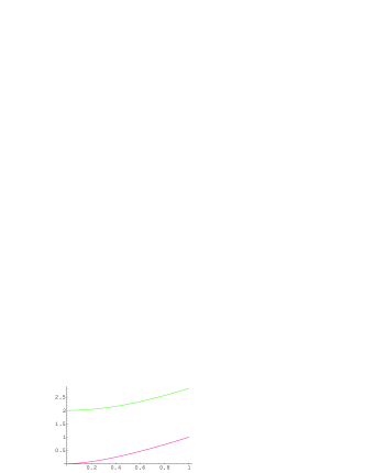
Figure 5: Plot of entanglement cost (${\cal E}$), given by eq. (19), and the maximal amount of violation of Bell inequality (${\cal B}$), given by eq. (20), against the visibility $V_{n}$ for the state $\chi_{path}$ obtained after the detection of the idlers in the entanglement swapping process with $n$ parametric down conversions.

We therefore obtain the important fact that the output state, resulting from a series of entanglement swappings, is always entangled and always violates local realism. Earlier works on entanglement swapping process via two parametric down converters ZZHE ; ZukowskiSwapProc made the tacit assumption that the output is a pure state admixed with white noise, and reached the conclusion that the swapped state is separable and does not violate local realism for low visibilities.

We will now discuss an interesting point with respect to violation of Bell inequalities of the state $\rho^{swap}_{path}$. Let us, for this state, find the $T$-matrix, whose elements for any state $\varrho$, of two qubits, is given by

$$T_{ij}=\mbox{tr}(\sigma_{i}\otimes\sigma_{j}\varrho),\quad(i,j=x,y,z).$$

In the above formula, we treat our qubits formally as spin-$1/2$ particles. For the state $\rho_{path}^{swap}$, $T_{xx}=V_{n}$, $T_{yy}=-V_{n}$, $T_{zz}=1$ and the rest are vanishing. A necessary and sufficient condition for a state of two qubits to violate local realism, for two settings per site, in the plane of $\vec{n}$ and $\vec{n}^{{}^{\prime}}$ is given by ZB

$$\sum_{i,j=\vec{n},\vec{n}^{{}^{\prime}}}T_{ij}^{2}>1.$$

In our case (i.e. for the state $\rho^{swap}_{path}$), $\sum_{i,j=x,y}T_{ij}^{2}=2V_{n}^{2}$, so that for $V_{n}>\frac{1}{\sqrt{2}}$, one obtains a violation of local realism in the $x-y$ plane. In the case of qubits defined by the output paths of the multiple entanglement swapping devices considered here, $x-y$ plane spin observables are equivalent to the measurement in the output ports of the external interferometers. That is, the $\vec{n}\cdot\vec{\sigma}$ operator for an $\vec{n}$ in the $x-y$ plane, is equivalent to a device consisting of a phase shifter in front of a 50-50 beamsplitter and two detectors behind it.

The $x-y$ plane does not provide a violation of local realism for $0\leq V_{n}\leq\frac{1}{\sqrt{2}}$, although the state is still entangled (and distillable) in that region. For these lower values of the visibility $V_{n}$, we have to consider other planes for obtaining a violation. For example in the $x-z$ plane, $\sum_{i,j=x,z}T_{ij}^{2}=1+V_{n}^{2}$, for the state $\rho^{swap}_{path}$, and thus a violation is always obtained in this plane. Hence, for these lower visibilities, one must use other measurement planes to obtain a violation. Such violation can therefore be obtained, only by the Mach-Zehnder interferometers at the output ports of the entanglement swapping device (Fig. 6). This is due to the fact that such a device is capable of performing any U(2) unitary transformation.

Figure 6: The schematic diagram shows that to obtain better violation of local realism, the output ports of the entanglement swapping (contained in the square box in the figure) should be put to the Mach-Zehnder interferometers.

For a wide range of pumps and filters used in the swapping process, one will have

$$b=c.$$

For example, this is the case when the pulse and filter functions are Gaussian, i.e.

$$F(\omega_{p})=\exp\{-\frac{(\omega_{p}-\omega_{0})^{2}}{2\sigma}\}$$ (21)

and

$$f(\omega_{p})=\exp\{-\frac{(\omega_{p}-\omega_{0}/2)^{2}}{2\sigma_{f}}\}.$$ (22)

In such cases, the normalized state created after the idlers have been detected in the multiple entanglement swapping process with $n$ PDCs is

$$\begin{array}[]{rcl}\rho^{swap}_{path}&=&\frac{1}{2}(\left|00\right\rangle\left\langle 00\right|+\left|11\right\rangle\left\langle 11\right|\\ &+&V_{n}^{(b=c)}\left|00\right\rangle\left\langle 11\right|+V_{n}^{(b=c)}\left|11\right\rangle\left\langle 00\right|),\end{array}$$

which can be rewritten as

$$\rho^{swap}_{path}=\frac{1+V_{n}^{(b=c)}}{2}\left|\phi^{+}\right\rangle\left\langle\phi^{+}\right|+\frac{1-V_{n}^{(b=c)}}{2}\left|\phi^{-}\right\rangle\left\langle\phi^{-}\right|$$

where $\left|\phi^{\pm}\right\rangle$ are the Bell states given by eq. (1).

One has to bear in mind that the above results were obtained under the asuumption that we deal with perfect entanglement swappings, especially no noise was allowed. It is obvious that for sufficiently low $V_{n}$ (see Fig. 5), both entanglement and violation of Bell inequalities would disappear, even for very minor noise admixtures.

Appendix A The two-photon state produced by PDC

This appendix is essentially meant to provide a “derivation” of the state (displayed in eqs. (2) and (3)) produced in a parametric down conversion. It is a reformulation of the theory of parametric down conversion which can be found in, e.g., Hong ; Mandelbook .

The phenomenon of spontaneous parametric down conversion (PDC) is a spontaneous fission of quasi monochromatic laser photons into correlated pairs of lower energy. All that takes place within a non-linear crystal. The probability of a single laser photon to fission is very low, but in a strong laser beam, the frequency of the phenomenon is quite high. The new photons, customarily called “signal” and “idler” have some basic properties. First of all, the wave vector ${\vec{k}}_{0}$ of the laser photons is related to those (${\vec{k}}_{i}$ and ${\vec{k}}_{s}$) of the idler and the signal by ${\vec{k}}_{0}\approx{\vec{k}}_{i}+{\vec{k}}_{s}$. One has to stress that this relation holds within the crystal (and can be thought of as an approximate conservation of the linear momentum). Secondly, the frequencies $\omega_{0}$, $\omega_{i}$, and $\omega_{s}$ of the laser photon, idler and signal satisfy $\omega_{o}\approx\omega_{i}+\omega_{s}$. And finally, the emerging pairs of photons are highly time-correlated. That is, if their optical paths from the source to the detectors are equal (which we assume in this paper), the detection times are equal too (up to the time resolution of the detection system). The relations between the wave vectors and between the frequencies are called phase matching conditions.

A.1 Crystal-field interaction.

Let us recall that in the interaction Hamiltonian of the electromagnetic field with an atom or molecule, the dominating part is $\hat{H}_{a-f}\sim\hat{\vec{\mu}}_{e}\cdot\vec{E}(\vec{x},t)$. That is, it is proportional to the scalar product of the dipole moment of the atom or molecule with the local electromagnetic field. Now the electric polarization of a material medium is given by the mean dipole moment of the atoms or molecules from which the medium is built (per unit volume). Let $\vec{p}(\vec{x},t)$ stand for the local polarization of the volume $\delta V$, which contains the point $\vec{x}$ (the volume $\delta V$ is macroscopically small but microscopically large). The principal term of the interaction Hamiltonian for crystal and field must have the form

$$H_{int}\sim\int_{V}\vec{p}(\vec{x},t)\cdot\vec{E}(\vec{x},t)d^{3}x,$$ (23)

where $V$ is the volume of the crystal. From the microscopic standpoint, the above formula reads

$$H_{int}\sim\int_{V}\sum_{n}\vec{\mu}_{n}\delta^{(3)}(\vec{x}-\vec{x}_{n})\cdot\vec{E}(\vec{x},t)d^{3}x,$$ (24)

where $\vec{x}_{n}$ is a symbolic representation of the position of the $n$-th atom endowed with a dipole moment $\vec{\mu}_{n}$. The summation is over all atoms (the word “atom” standing for any stable aggregate of charged particles, like atoms themselves, or ions, or molecules) of the medium. One can see that the formula (24) agrees with $\hat{H}_{a-f}$. If one introduces the averaged (macroscopic) polarization (averaged over the macroscopically small volumes $\delta V$), we get (23). One can assume that $\vec{E}(\vec{x},t)$ interacts with $\vec{p}(\vec{x},t)$ only in the point $\vec{x}$, thus the $i$-th component of polarization is in the most general case given by

$$\begin{array}[]{rcl}p_{i}(\vec{x},t)&=&\sum_{j=1}^{3}\chi_{ij}^{(1)}(\vec{x})E_{j}(\vec{x},t)\\ &+&\sum_{j,k=1}^{3}\chi_{ijk}^{(2)}(\vec{x})E_{j}(\vec{x},t)E_{k}(\vec{x},t)+\cdots,\end{array}$$ (25)

where $\chi_{ij}^{(1)}$ are $\chi_{ijk}^{(2)}$ are the (macroscopic) polarizability coefficients. They are in the form of tensors. This is due to the fact that polarizablility may depend on the polarization of the incoming light. Note here that for any crystal which is built of molecules which are centro-symmetric the quadratic term of the polarizability vanishes. Therefore the effect exists only in birefringent media.

In the case of a perfect “nonlinear” crystal, we assume that $\chi_{ijk}^{(2)}(\vec{x})$ has the same value for all point within the crystal. The nonlinear term of the polarization gives the following term in the interaction Hamiltonian (cf. (23)):

$$\begin{array}[]{lcl}&&H_{int}\sim\int_{V}\vec{p}(\vec{x},t)\cdot\vec{E}(\vec{x},t)d^{3}x\\ &&=\int_{V}\vec{p}^{\>lin}(\vec{x},t)\cdot\vec{E}(\vec{x},t)d^{3}x\\ &&+\int_{V}\vec{p}^{\>non}(\vec{x},t)\cdot\vec{E}(\vec{x},t)d^{3}x,\end{array}$$

where $\vec{p}^{\>lin}$ ($\vec{p}^{\>non}$) is the linear (nonlinear) term of polarization. The nonlinear part of the Hamiltonian is

$$H^{NL}\sim\int_{V}\sum_{ijk}\chi_{ijk}^{(2)}E_{i}(\vec{x},t)E_{j}(\vec{x},t)E_{k}(\vec{x},t)d^{3}x.$$ (26)

The quantized field can be expressed (in the interaction picture) as

$$\begin{array}[]{lcl}&&\vec{E}(\vec{x},t)=\sum_{p=1}^{2}\int\>d^{3}k\frac{i}{\sqrt{2\omega(2\pi)^{3}}}\times\\ &&\hat{\epsilon}(\vec{k},p)a^{-}(\vec{k},p)\exp\{i(\vec{k}\cdot\vec{x}-\omega t)\}+h.c.\\ &&=\vec{E}^{(+)}(\vec{x},t)+\vec{E}^{(-)}(\vec{x},t),\end{array}$$ (27)

where $\vec{E}^{(-)}(\vec{x},t)=[\vec{E}^{(+)}(\vec{x},t)]^{\dagger}$, and the summation is over two orthogonal linear polarizations, $h.c$ denotes the hermitian conjugate of the previous term, $\hat{\epsilon}(\vec{k},p)$ is a unit vector defining the linear polarization. The symbol $a^{-}(\vec{k},p)$ stands for the annihilation operator of a photon of a wave vector $\vec{k}$ and polarization $\hat{\epsilon}(\vec{k},p)$. The principal commutation rule for the creation and annihilation operators is given by $[a(\vec{k},p),a^{\dagger}(\vec{k}^{\prime},p^{\prime})]=\delta_{p,p^{\prime}}\delta^{(3)}(\vec{k}-\vec{k}^{\prime})$, $[a^{\dagger}(\vec{k},p),a^{\dagger}(\vec{k}^{\prime},p^{\prime})]=0$ and $[a(\vec{k},p),a(\vec{k}^{\prime},p^{\prime})]=0$ . As we are interested only in the PDC process, we will neglect the depletion of the laser field and assume that the total field within the crystal is $\vec{E}(\vec{x},t)=\vec{E}^{Laser}(\vec{x},t)+\vec{E}_{q}(\vec{x},t)$, where the laser beam is described by a classical electromagnetic field $\vec{E}^{Laser}$. In reality, the laser field is a mixture of coherent states, and its phase is undefined, but this is of no consequence to us here. The field $\vec{E}_{q}$ is described in a quantum-electrodynamical way. It describes the secondary photons emitted by the crystal. The down conversion takes place, thanks to the terms in (26) of the form $\int_{V}\sum_{ijk}\chi_{ijk}^{(2)}E_{i}^{Laser}E_{j}E_{k}d^{3}x$. Only those terms of $E_{j}$ and $E_{k}$ which contain the creation operators, can give rise to a two photon state, after acting on the vacuum state $|\Omega\rangle$. The creation operators can be found only in the so-called negative frequency terms of the electromagnetic field operators (that is, in those which contain the factors $\exp\{-i(\vec{k}\cdot\vec{x}-\omega t)\}$ (cf. (27))). Let us therefore forget about all other terms and analyze only

$$H^{NL}\sim\int_{V}\sum_{ijk}\chi_{ijk}^{(2)}E_{i}^{Laser}E_{j}^{(-)}E_{k}^{(-)}d^{3}x+\mbox{h.c.}$$ (28)

For simplicity let us describe the laser field as a monochromatic wave $\vec{E}_{Laser}(\vec{x},t)=\hat{x}E_{0}(\exp\{i(\vec{k_{0}}\cdot\vec{x}-\omega_{0}t-\phi)\}+c.c)$, where $2E_{0}$ is the field amplitude and $c.c$ denotes the complex conjugate of the previous expression. (Since an arbitrary electromagnetic field is a superposition of the plane waves, it is very easy to get the general description.) Then from (28), one gets

$$\begin{array}[]{lcl}&&H^{NL}\sim\int_{V}\sum_{jk}\{\chi_{3jk}^{(2)}E_{0}\times\\ &&[\exp\{i(\vec{k}_{0}\cdot\vec{x}-\omega_{0}t-\phi)\}+c.c]\times\\ &&\sum_{p}\int d^{3}k\>f(\omega)\hat{\epsilon}(\vec{k},p)a^{\dagger}(\vec{k},p)\exp\{-i\vec{k}\cdot\vec{x}\}\times\\ &&\sum_{p^{\prime}}\int d^{3}k^{\prime}\>f(\omega)\hat{\epsilon}(\vec{k},p)a^{\dagger}(\vec{k}^{\prime},p)\exp\{-i\vec{k^{\prime}}\cdot\vec{x}\}d^{3}x\\ &&+\mbox{h.c.},\end{array}$$ (29)

with $f(\omega)$ being a factor dependent on $\omega$. Its specific structure is irrelevent here. Extracting only those elements of the above expression which contain $\vec{x}$, one sees that their overall contribution to (29) is given by $\int_{V}d^{3}x\>\exp\{i\vec{x}(\pm\vec{k}_{0}-\vec{k}-\vec{k}^{\prime})\}$, which we write as $\Delta(\vec{k}_{0}-\vec{k}-\vec{k}^{\prime})$. If we assume that our crystal is a cube $L\times L\times L$, then for $L\rightarrow\infty$, $\Delta$ approaches the Dirac delta $\delta(\pm\vec{k}_{0}-\vec{k}-\vec{k}^{\prime})$. Thus, we immediately conclude that the emission of the pairs of photons is possible only for the directions for which the condition $\vec{k}_{0}\approx\vec{k}+\vec{k}^{\prime}$ is met footnote1 . Eq. (29) can be therefore put in the form

$$\begin{array}[]{lcl}&&H^{NL}\sim\sum_{p,p^{\prime}}\int d^{3}k\int d^{3}k\Delta(\vec{k}_{0}-\vec{k}-\vec{k}^{\prime})A^{eff}_{p,p^{\prime}}\times\\ &&\exp\{-i\omega_{0}t\}a^{\dagger}(\vec{k},p)a^{\dagger}(\vec{k}^{\prime},p^{\prime})+\mbox{h.c},\end{array}$$ (30)

where $A^{eff}_{p,p^{\prime}}=\sum_{j,k}E_{0}\chi_{3jk}^{(2)}\hat{\epsilon}_{j}(\vec{k},p)\hat{\epsilon}_{k}(\vec{k}^{\prime},p^{\prime})$ is the effective amplitude of the laser pump field (which serves as a laser-crystal coupling strength). This Hamiltonian fully describes the basic traits of the phenomenon of down conversion. In the so called type II down conversion, the laser pump beam is ordinary wheras the idler and signal photons are extraordinary. Thus we shall replace the general $A^{eff}_{p,p^{{}^{\prime}}}$ by $F_{0}$.

A.2 The state of photons emitted in the PDC process.

We are interested in the process of production of pairs of photons. Therefore we shall assume that the pump field is rather weak, so that the events of double pairs emissions are very rare. Therefore one can use the perturbation theory.

The evolution of the state $\left|\Psi_{D}(t)\right\rangle$ (in the interaction (Dirac) picture) of the photons emitted in the PDC process is governed by the Schrödinger equation $i\hbar\frac{d}{dt}|\Psi_{D}(t)\rangle=H^{NL}_{D}(t)|\Psi_{D}(t)\rangle$, where $H^{NL}_{D}(t)=\exp\{\frac{i}{\hbar}H_{0}t\}H^{NL}\exp\{-\frac{i}{\hbar}H_{0}t\}$, and $H_{0}+H^{NL}$ is the total Hamiltonian of the system. Therefore

$$\begin{array}[]{rcl}|\Psi_{D}(t)\rangle&=&|\Psi_{D}(t_{0})\rangle+\frac{1}{i\hbar}\int_{t_{0}}^{t}H^{NL}_{D}(t^{\prime})|\Psi_{D}(t^{\prime})\rangle dt^{\prime}\\ &\simeq&|\Psi_{D}(t_{0})\rangle+\frac{1}{i\hbar}\int_{t_{0}}^{t}H^{NL}_{D}(t^{\prime})|\Psi_{D}(t_{0})\rangle dt^{\prime},\end{array}$$ (31)

where we have replaced the time dependent state in the integral by its initial form $|\Psi_{D}(t_{0})\rangle$ using the first order of the perturbation calculus. In the Dirac picture, the creation and annihilation operators depend on time as $a_{D}^{\dagger}(\vec{k},p,t)=\exp\{i\omega t\}a^{\dagger}(\vec{k},p)$ and $a_{D}(\vec{k},p,t)=\exp\{i\omega t\}a(\vec{k},p)$. In (31), we put $t_{0}=0$, and we take the vacuum state (no photons) $|\Omega\rangle$ as the initial state $|\Psi(0)\rangle$. We are interested only in the term with the integral, because it is only there that one can find creation operators responsible for the spontaneous emission of pairs of photons. The photons interact with the laser field only during the time of the order of $\frac{L}{c}$. The interaction simply ceases when they leave the crystal. Therefore, as the annihilation operators when acting on the vacuum state give zero, one can write

$$\begin{array}[]{lcl}&&\sum_{p,p^{\prime}}\int d^{3}k\int d^{3}k^{{}^{\prime}}F_{0}\Delta(\vec{k}_{0}-\vec{k}-\vec{k}^{\prime})\Delta(\omega+\omega^{\prime}-\omega_{0})\\ &&a^{\dagger}(\vec{k},p)a^{\dagger}(\vec{k}^{\prime},p^{\prime})|\Omega\rangle,\end{array}$$

where we have written $\int_{0}^{\frac{L}{c}}dt^{\prime}\exp\{it^{\prime}(\omega+\omega^{\prime}-\omega_{0})\}$ as $\Delta(\omega+\omega^{\prime}-\omega_{0})$. As $L\rightarrow\infty$, $\Delta$ behaves as a Dirac delta. Thus the allowed frequencies of the emissions satisfy the relation footnote2 $\omega_{0}\approx\omega+\omega^{\prime}$. Since $\frac{L}{c}\omega$, $\frac{L}{c}\omega^{\prime}$ and $\frac{L}{c}\omega_{0}$ are typically of the order of $10^{4}$ the function $\Delta(\omega+\omega^{\prime}-\omega_{0})$ is very close to $\delta(\omega+\omega^{\prime}-\omega_{0})$.

A.3 Directions of emissions

We know that $\omega=|\vec{k}|\frac{c}{n(\omega,p)}$, where $\frac{c}{n(\omega,p)}=c(\omega,p)$ is the speed of light in the given medium, which depends on frequency and the polarization. Using this relation as well as phase matching condition for frequencies, we get the condition $|\vec{k}_{0}|c(\omega_{0})\simeq|\vec{k}|c(\omega,p)+|\vec{k}^{\prime}|c(\omega^{\prime},p^{\prime})$. Therefore, the emissions of the pairs are possible only when the phase matching and the above condition are both met. This means that the correlated emissions occur only for specific directions, specific frequencies and specific polarizations. There are two types of down conversions:

1. both photons of a pair have the same polarization (type I),

2. they have orthogonal polarizations (type II).

Additionally if one has:

1. $\omega\simeq\omega^{\prime}$ then we have a frequency degenerate PDC,

2. and if $\hat{k}=\hat{k}^{\prime}$, then we have a co-linear one.

A.4 Time correlations

In this section it will be shown that the down converted photons are very tightly time correlated. The probability of a detection of a photon, of say, the horizontal polarization $H$, at a detector situated at point $\vec{x}$ and at the moment of time $t$, is proportional to

$$p(\vec{x},t,H)\simeq\eta Tr\varrho E_{H}^{(-)}(\vec{x},t)E_{H}^{(+)}(\vec{x},t),$$ (32)

where $\eta$ is the coefficient which characterizes the quantum efficiency of the detection process, $\varrho$ is the density operator, which represents the field in the Heisenberg picture, $E_{H}$ is the horizontal component of the field in the detector. For the above relation to be true, we also assume that via the aperture of the detector enter only photons of a specified direction of the wave vector.

For a pure state, (32) reduces to $p(\vec{x},t,H)\simeq\langle\psi|E_{H}^{(-)}E_{H}^{(+)}|\psi\rangle$. The probability of a joint detection of two photons, of polarization $H$, at the locations $\vec{x}_{1}$ and $\vec{x}_{2}$, and at the moments of time $t_{1}$ and $t_{2}$ is proportional to

$$\begin{array}[]{lcl}&&p(\vec{x}_{1},t_{1};\vec{x}_{2},t_{2})\sim\\ &&\langle\psi|E_{H}^{(-)}(\vec{x}_{1},t_{1})E_{H}^{(-)}(\vec{x}_{2},t_{2})E_{H}^{(+)}(\vec{x}_{2},t_{2})E_{H}^{(+)}(\vec{x}_{1},t_{1})|\psi\rangle.\end{array}$$ (33)

The evolution of the field within the crystal lasts for the time around $\frac{L}{c}$. If the detectors are very far away from each other, and from the crystal, then the photon field can be treated as free-evolving. State $|\psi\rangle$ is the photon state that leaves the crystal at the moment around $\frac{L}{c}$:

$$|\psi(t=\frac{L}{c})\rangle=|\Omega\rangle+\frac{1}{i\hbar}e^{-\frac{i}{\hbar}H_{0}\frac{L}{c}}\int_{0}^{\frac{L}{c}}H_{D}^{NL}(t^{\prime})dt^{\prime}|\Omega\rangle.$$ (34)

Let $t=t_{1}$ i $t_{2}=t^{\prime}$, and $|\psi\rangle=|\psi(t=\frac{L}{c})\rangle$, then (33) can be written down as

$$\begin{array}[]{lcl}&&p(\vec{x}_{1},t|\vec{x}_{2},t^{\prime})\simeq\\ &&\langle\psi|E_{H}^{(-)}(\vec{x}_{1},t)E_{H}^{(-)}(\vec{x}_{2},t^{\prime})E_{H}^{(+)}(\vec{x}_{1},t)E_{H}^{(+)}(\vec{x}_{2},t^{\prime})|\psi\rangle.\end{array}$$ (35)

If we choose just two conjugate propagation directions (i.e. such that fulfill the phase-matching conditions), then approximately one has

$$\begin{array}[]{rcl}E_{H}^{(+)}(\vec{x},t)&=&\int d\omega e^{-i\omega t}f_{1}(\omega)a_{1}(\omega)\\ E_{H}^{(+)}(\vec{x}^{\prime},t^{\prime})&=&\int d\omega e^{-i\omega t^{\prime}}f_{2}(\omega)a_{2}(\omega),\end{array}$$

where $f_{1}$ and $f_{2}$ are the frequency response function which characterize the detections (or rather filter-detector system). We assume that the response functions are such that their maxima agree with the frequencies determined by the phase-matching conditions. The annihilation and creation operators which were used above, are replaced by $a_{i}(\omega)$ and its conjugate, which can be used to describe “unidirectional” excitations of the photon field (i.e., we assume that the detectors see only the photons of a specified duration of propagation, this a good assumption if the detectors are far from the crystal, and the apertures are narrow). The index $i$ defines the direction (fixed) of the wave vector. The operators satisfy commutation relation, which are a modification of those given above to the current specific case $[a_{i}(\omega),a^{\dagger}_{j}(\omega^{\prime})]=\delta_{ij}\delta(\omega-\omega^{\prime})$, $[a_{i}(\omega),a_{j}(\omega^{\prime})]=0$.

Introducing an unit operator $\hat{I}=\sum_{i=0}^{\infty}|b_{i}\rangle\langle b_{i}|$, where $|b_{i}\rangle$ is a basis state into (35), we obtain

$$\begin{array}[]{lcl}&&p(\vec{x}_{1},t|\vec{x}_{2},t^{\prime})\simeq\\ &&\langle\psi|E_{H}^{(-)}(\vec{x}_{1},t)E_{H}^{(-)}(\vec{x}_{2},t^{\prime})\hat{I}E_{H}^{(+)}(\vec{x}_{1},t)E_{H}^{(+)}(\vec{x}_{2},t^{\prime})|\psi\rangle.\end{array}$$ (36)

Since $E_{H}^{(+)}$ contains only the annihilation operators, they transform the two photon state $|\Psi\rangle$ into the vacuum state. Thus, the equation (36) can be written down as

$$p(\vec{x}_{1},t|\vec{x}_{2},t^{\prime})\simeq\langle\psi|E_{H}^{(-)}E_{H}^{{}^{\prime}(-)}|\Omega\rangle\langle\Omega|E_{H}^{(+)}E_{H}^{{}^{\prime}(+)}|\psi\rangle,$$ (37)

where the primed expressions pertain to the moment of time $t^{\prime}$ and the position $\vec{x}_{2}$. Thus we have $p(\vec{x}_{1},t|\vec{x}_{2},t^{\prime})\simeq|A_{12}(t,t^{\prime})|^{2}$, where $A_{12}(t,t^{\prime})=\langle\Omega|E_{H}^{(+)}(\vec{x}_{1},t)E_{H}^{{}^{\prime}(+)}(\vec{x}_{2},t^{\prime})|\psi\rangle$. The state $|\Psi\rangle$ can be approximated by

$$|\Psi\rangle=|\Omega\rangle+\int d\omega_{1}\int d\omega_{2}F_{0}\delta(\omega-\omega_{1}-\omega_{2})a^{\dagger}_{1}(\omega_{1})a^{\dagger}_{2}(\omega_{2})|\Omega\rangle.$$ (38)

Then

$$\begin{array}[]{lcl}&&A_{12}(t,t^{\prime})=\langle\Omega|\int d\omega^{\prime}e^{-i\omega^{\prime}t}f_{2}(\omega^{\prime})a_{2}(\omega^{\prime})\\ &&\int d\omega e^{-i\omega t}f_{1}(\omega)a_{1}(\omega)\int d\omega_{2}\int d\omega_{2}F_{0}\delta(\omega_{0}-\omega_{1}-\omega_{2})\\ &&a_{2}^{\dagger}.(\omega_{2})a_{1}^{\dagger}(\omega_{1})|\Omega\rangle\end{array}$$

Since the creation and annihilation operators for different modes commute, and since one can use $\langle\Omega|a_{i}(\omega^{\prime})a_{j}^{\dagger}(\omega)|\Omega\rangle=\delta_{ij}\delta(\omega^{\prime}-\omega)$, we get

$$A_{12}(t,t^{\prime})=e^{-i\omega_{0}t^{\prime}}\int d\omega F_{0}e^{-i\omega(t-t^{\prime})}f_{2}(\omega_{0}-\omega)f_{1}(\omega).$$ (39)

If $F_{0}$ varies very slowly, which is a good asumption in the case of a crystal, then we have

$$\begin{array}[]{lcl}&&p(\vec{x}_{1},t|\vec{x}_{2},t^{\prime})\sim|A_{12}(t,t^{\prime})|^{2}\\ &&\simeq|\int d\omega e^{-i\omega(t-t^{\prime})}f_{2}(\omega_{0}-\omega)f_{1}(\omega)|^{2}.\end{array}$$ (40)

We see that the probability will depend on the difference of the detection times.

To illustrate the above, let us assume that $f_{1}=f_{2}=f$, and that they are gaussian. Then, if one assumes that the central frequency of $f$ is $\omega_{c}=\frac{1}{2}\omega_{0}$ and $f(\omega)=Ce^{-\frac{(\omega_{c}-\omega)^{2}}{{\sigma}^{2}}}$, then we have $f_{1}(\omega)=f_{2}(\omega_{0}-\omega)=f(\omega)$. If one uses these relations the probability of detection of two photons at the moments $t$ and $t^{\prime}$ satisfies the following dependence

$$\begin{array}[]{lcl}&&p(\vec{x}_{1},t|\vec{x}_{2},t^{\prime})\\ &&\sim|\int d\omega e^{-i\omega(t-t^{\prime})}C^{2}e^{-2\frac{{(\omega_{c}-\omega)}^{2}}{{\sigma}^{2}}}|^{2}\sim e^{-\frac{\sigma^{2}}{2}(t-t^{\prime})^{2}}.\end{array}$$ (41)

We see, that if $\sigma\rightarrow\infty$ (that is, the detector has an infinitely broad frequency response) then the expression (41) approaches the Dirac delta $\delta(t-t^{\prime})$ and this means, that the two detectors register the two photons at the same moment of time. However, such detectors do not exist. Nevertheless, from equations (40) and (41), we see that the degree of time correlation of the detection of the PDC photons depends on the frequency response of the detectors. Thus, the photons are almost perfectly time correlated.

We have shown what are the reasons for the properties of the PDC photons. Although the above reasoning was done under the assumption of a monochromatic nature of the pumping field, all this can be generalized to the non-monochromatic case, including the most interesting one of a pulsed pump. The distinguishing traits of this situation can be summarized by the following remarks. The emission from the crystal can appear only when the pulse is within the crystal. Further, the frequency $\omega_{0}$ and the wave vector are not strictly defined. If the pulse is too short because of the relation $T\approx\frac{1}{\Delta\omega}$, where $T$ is the pulse width, the PDC photons are less tightly correlated directionally.

The two photon state coming out of a PDC can then be approximated by

$$\begin{array}[]{lcl}|\Psi\rangle=&&\int d\omega_{0}F(\omega_{0})\int d\omega_{1}\int d\omega_{2}\times\\ &&\Delta(\omega_{0}-\omega_{1}-\omega_{2})a^{\dagger}_{1}(\omega_{1})a^{\dagger}_{2}(\omega_{2})|\Omega\rangle,\end{array}$$ (42)

where we have replaced the effective pump amplitude by the spectral decomposition of the laser pulse $F(\omega_{0})$. Since a pulse is a superposition of monochromatic waves, we therefore integrate over the spectrum.

References

- (1) M. Żukowski, A. Zeilinger, M.A. Horne and A.K. Ekert, Phys. Rev. Lett. 71, 4287 (1993).
- (2) S. Bose, V. Vedral, and P.L. Knight, Phys. Rev. A 57, 822 (1998); ibid. 60, 194 (1999).
- (3) C.H. Bennett, G. Brassard, C. Crepeau, R. Josza, A Peres, and W.K. Wootters, Phys. Rev. Lett. 70, 1895 (1993).
- (4) J.-W. Pan, D. Bowmeester, H. Weinfurter, and A. Zeilinger, Phys. Rev. Lett. 80, 3891 (1998).
- (5) M. Żukowski, A. Zeilinger, and H. Weinfurter, Annals N.Y. Acad. Sci. 755, 91 (1995).
- (6) H.-J. Briegel, W. Dür, J.I. Cirac, and P. Zoller, Phys. Rev. Lett. 81, 5932 (1998); W. Dür, H.-J. Briegel, J.I. Cirac, and P. Zoller, Phys. Rev. A 59, 169 (1999).
- (7) C.H. Bennett, D.P. DiVincenzo, J.A. Smolin, and W.K. Wootters, Phys. Rev. A 54, 3824 (1996).
- (8) A. Zeilinger, M.A. Horne, H. Weinfurter, and M. Żukowski, Phys. Rev. Lett. 78, 3031 (1997).
- (9) We shall not discuss here the effects linked with the statistics of the output of the PDC sources.
- (10) The partial transpose of a bipartite state , where and are the indices for party and and are the indices for party , with respect to part is Peres1 . A state is said to have positive partial transpose if is a positive operator. has non-positive partial transpose otherwise. A state with non-positive partial transpose is always entangled Peres1 .
- (11) A. Peres, Phys. Rev. Lett 77 1413 (1996).
- (12) M. Horodecki, P. Horodecki, and R. Horodecki, Phys. Lett. A 223, 1 (1996).
- (13) S. Hill and W.K. Wootters, Phys. Rev. Lett. 78, 5022 (1997); W.K. Wootters, Phys. Rev. Lett. 80, 2245 (1998).
- (14) G. Vidal, W. Dür, and J.I. Cirac, Phys. Rev. Lett. 89, 027901 (2002).
- (15) M. Horodecki, A. Sen(De), and U. Sen, The rates of asymptotic entanglement transformations for bipartite mixed states: Maximally entangled states are not special, to appear in Phys. Rev. A (quant-ph/0207031).
- (16) P.W. Shor, J. Math. Phys. 43, 4334 (2002).
- (17) M. Horodecki, P. Horodecki, and R. Horodecki, Phys. Rev. Lett. 78, 574 (1997).
- (18) E.M. Rains, Phys. Rev. A 60, 179 (1999); E.M. Rains, Phys. Rev. A 63, 019902 (2001); E.M. Rains, A semidefinite program for distillable entanglement, quant-ph/0008047.
- (19) E.M. Rains, Phys. Rev. A 60, 173 (1999) .
- (20) J.S. Bell, Physics 1, 195 (1964).
- (21) R. Horodecki, P. Horodecki, and M. Horodecki, Phys. Lett. A 200, 340 (1995).
- (22) M. Żukowski and Č. Brukner, Phys. Rev. Lett. 88, 210401 (2002).
- (23) C.K. Hong and L. Mandel, Phys. Rev. A 31, 2409 (1985).
- (24) L. Mandel and E. Wolf, Optical Coherence and Quantum Optics, Cambridge University Press (1995).
- (25) The condition with the minus sign in the delta function cannot be met because in this case the phase matching condition for the frequancies cannot be satisfied.
- (26) Note here that if we had kept in the Hamiltonian the terms for which , then the condition for frequencies would have emerged (cf. Ref. footnote1 ), and this is impossible to meet!