Quantum phase estimation algorithms with delays: effects of dynamical phases

Abstract

The unavoidable finite time intervals between the sequential operations needed for performing practical quantum computing can degrade the performance of quantum computers. During these delays, unwanted relative dynamical phases are produced due to the free evolution of the superposition wave-function of the qubits. In general, these coherent “errors” modify the desired quantum interferences and thus spoil the correct results, compared to the ideal standard quantum computing that does not consider the effects of delays between successive unitary operations. Here, we show that, in the framework of the quantum phase estimation algorithm, these coherent phase “errors”, produced by the time delays between sequential operations, can be avoided by setting up the delay times to satisfy certain matching conditions.

PACS number(s): 03.67.Lx

I Introduction

Building a prototype quantum information processor has attracted considerable interest during the past decade (see, e.g., Nielsen00 ). This desired device should be able to simultaneously accept many different possible inputs and subsequently evolve them into a corresponding quantum mechanical superposition of outputs. The proposed quantum algorithms are usually constructed for ideal quantum computers. In reality, any physical realization of such a computing process must treat various errors arising from various noise and imperfections (see, e.g., Nielsen00 ; Mussinger00 ; Long ). Physically, these errors can be distinguished into two different kinds: incoherent and coherent errors. The incoherent perturbations, originating from the coupling of the quantum computer to an uncontrollable external environment, result in decoherence and stochastic errors. Coherent errors usually arise from non-ideal quantum gates which lead to a unitary but non-ideal temporal evolution of the quantum algorithm. So far, almost all previous works (see, e.g., Shor95 ; Steane98 ; Lidar98 ; Zanardi97 ) have been concerned with quantum errors arising from the decoherence due to interactions with the external environment and external operational imperfections. Here, we will not be concerned with these two types of externally-induced errors, but will focus instead on intrinsic ones. The coherent errors we consider here relate to the intrinsic dynamical evolution of the qubits between operations. This has not been paid much attention until a recent work in Berman00 , where a kind of dynamical phase error was introduced. It is well-known that a practical quantum computing process usually consists of a number of sequential quantum unitary operations. These transformations operate on superposition states and evolve the quantum register from the initial states (input) into the desired final states (output). According to the Schrödinger equation, the superposition wave function oscillates fast during the finite-time delay between two sequential operations. In general, these oscillations modify the desired quantum interferences and thus spoil the correct computational results, expected by the ideal quantum algorithms without any operational delay.

Two different strategies have been proposed to deal with these coherent errors. One is the so-called “avoiding error” approach proposed by Makhlin et al in Ref. MSS99 . Its key idea is to let the Hamiltonian of the bare two-level physical system be zero by properly setting up experimental parameters. Thus the system does not evolve during the delays. This requirement is restrictive and cannot be easily implemented for some physical setups of quantum computing e.g., for trapped ions. A modified approach to remove this stringent condition was proposed by Feng in Ref. Feng01 , where a pair of degenerate quantum states of a pair of two-level systems are used to encode two logic states of a single qubit. During the delay these logical states acquire a common dynamical phase, which is the global phase without any physical meaning. Thus the above dynamical error can be avoided efficiently. However, this modified scheme complicates the process of encoding information. Another strategy to this problem was proposed by Berman et al. Berman00 . They pointed out that the unwanted dynamical oscillations can be routinely eliminated by introducing a “natural” phase, which can be induced by using a stable continuous reference oscillation for each quantum transition in the computing process. However, this scheme only does well for the resonant implementations of quantum computation. The additional reference pulses also complicate the quantum computing process and may result in other operational errors.

We show in this paper that, in the framework of the quantum phase estimation algorithm, the coherent phase errors, produced by the free evolutions of the superposition wave functions of bare two-level systems, can be avoided simply and effectively by setting up the delay time intervals appropriately. The proposed matching condition can be considered a sort of strobed operation (with strobe frequencies corresponding to each different transition energy). For simplicity, we simplify each quantum algorithm to a three-step functional process, namely: preparation, evolution, and measurement. All the functional operations in this three-step process are assumed to be carried out in an infinitesimally short time duration, and thus only the delays between them, instead of the operations themselves, are considered. The effects of the environment decoherence and the operational imperfections are neglected in the present treatment.

The paper is organized as follows. In Section II, we present our general approach with the phase estimation algorithm. Sec. III gives a few special demonstrations and shows how to perform quantum order-finding and quantum counting algorithms in the presence of operational delays. Finally, we give a short summary and discussion in Sec. IV.

II Phase estimation algorithm with operational delays

Our discussion begins with the phase estimation algorithm Kitaev95 ; Cleve98 and its finite-time implementation with some delays. The programs for some of the existing other important quantum algorithms, such as quantum factoring and counting ones, can be reformulated in terms of this problem. The goal of the phase estimation algorithm is to obtain an $n-$bit estimation of the eigenvalue $\exp(i\phi)$ of a unitary operation $\hat{U}_{T}$,

$$\hat{U}_{T}\,|\phi\rangle_{T}=e^{i\phi}\,|\phi\rangle_{T},$$ (1)

if the corresponding eigenvector $|\phi\rangle_{T}$, and the devices that can perform operations $\hat{U}_{T}$, $\hat{U}^{2}_{T}$, $\hat{U}_{T}^{4},\cdots$, and $\hat{U}^{2^{n}}_{T}$, are given initially. Two quantum registers are required to perform this algorithm. One is the target register, whose quantum state is kept in the eigenstate $|\phi\rangle_{T}$ of the unitary operator $\hat{U}_{T}$. Another one, with $n$ physical qubits and called the index register, is used to read the corresponding estimation results. The needed number of qubits $n$ in the index register depends on the desired accuracy and on the success probability of the algorithm. The most direct application Abrams99 of this algorithm is to find eigenvalues and eigenvectors of a local Hamiltonian $\hat{H}_{T}$ by determining the time-evolution unitary operator $\hat{U}_{T}=\exp(-i\hat{H}_{T}t/\hbar)$. The phase estimation algorithm can be viewed as a quantum nondemolition measurement, and can also be used to generate eigenstates of the corresponding unitary operator $\hat{U}_{T}$ Travaglione02 .

The ideal quantum algorithm usually assumes that the quantum computing process can be continuously performed by using a series of sequential operations without any time-delay between them. In reality, a delay between two sequential operations always exists, introducing errors that need to be corrected. For simplicity, we reduce the phase estimation algorithm to a three-step functional process, namely: initialization, global phase shift, and measurement. All the functional operations in this three-step process are assumed to be carried out exactly, and thus only the delays between them, instead of the operations themselves, are considered. Such a simplified finite-time implementation of the phase estimation algorithm is sketched in Fig. 1. For convenience we distinguish the physical qubit and the logic qubit in the index register. The physical qubit is just a two-level physical system and the logical qubit is the unit of binary information. Unlike the scheme in Feng01 , wherein two physical qubits are used to encode one logical qubit, in the present work one physical qubit is enough to encode one logical qubit. The symbol $|a_{j}\rangle_{k}$ with $a=0,1,\,\,j,k=0,1,...,n-1$ means that the $k$th logical qubit is encoded by the $j$th physical qubit. $|a_{j}\rangle$ is the eigenstate of the bare Hamiltonian of the $j$th physical qubit corresponding to the eigenvalue $E_{a}$.

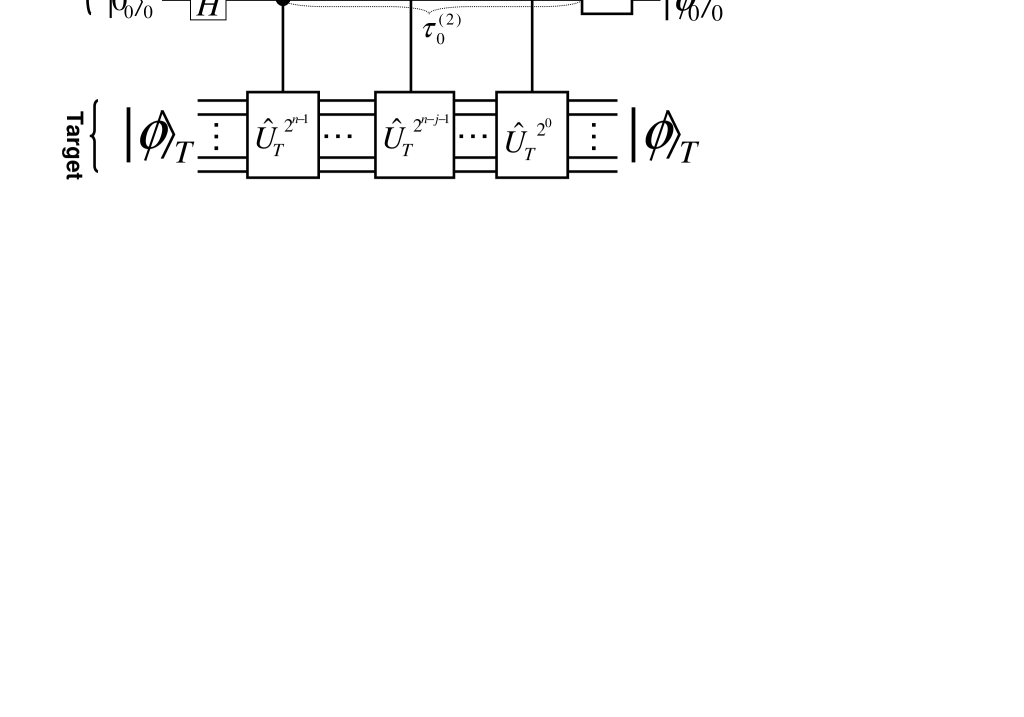
Figure 1: Quantum phase estimation with operational delays. Note that: 1) there is an operational delay $\tau_{j}^{(m)}(m=1,2)$ between successive quantum operations on the $j$th physical qubit, and 2) the $j$th logical qubit is changed to the $(n-j-1)$th one after the Hadamard gate $\hat{H}$ and inverse QFT $\hat{F}^{-1}$. Here, $\tau^{(1)}_{j}$ is time delay between the $\hat{H}$ and $\hat{U}_{T}^{2^{n-j-1}}$ operations, while $\tau^{(2)}_{j}$ is the delay between $\hat{U}_{T}^{2^{n-j-1}}$ and $\hat{F}^{-1}$.

The quantum phase estimation algorithm with operational delays can be divided into three distinct functional steps:

II.1 Initialization

First, we initialize the index register with $n$ physical qubits in an equal-weight superposition of all logical states. This can be performed by applying the Hadamard transform to its ground state $|0\rangle_{I}=\prod_{j=n-1}^{0}|0\rangle_{j}.$ Note that the target register holds an eigenstate $|\phi\rangle_{T}$ of $\hat{U}_{T}$ with eigenvalue $\exp(i\phi)$. Hereafter, the sub-index $I$ will denote the index state, while the subindex $T$ refers to the target state. The computational initial state of the whole system is

$$|\Psi(0)\rangle=\left\{\prod_{j=n-1}^{0}\hat{H}_{j}\,|0_{j}\rangle_{j}\right\}_{I}\otimes|\phi\rangle_{T}=\frac{1}{\sqrt{2^{n}}}\sum_{k=0}^{2^{n}-1}|k\rangle_{I}\otimes|\phi\rangle_{T},\,\,\,\hat{H}_{j}=\frac{1}{\sqrt{2}}\left(\begin{array}[]{cc}1&1\\ 1&-1\end{array}\right)_{j},$$ (4)

where $|k\rangle_{I}=|a_{0}\rangle^{k}_{n-1}\otimes\cdots\otimes|a_{n-1}\rangle^{k}_{0}$ are the number states of the index register, and $\hat{H}_{j}$ is the Hadamard transform applied to the $j$th logical qubit. For convenience, in this paper the $j$th logical qubit is changed into the $(n-1-j)$th logical qubit when applying either the Hadamard or the (inverse) quantum Fourier transform (QFT). Of course, the order of the physical qubits is not changed.

After a finite time delay $\tau^{(1)}_{j}$ for the $j$th physical qubit, the initial state $|\Psi(0)\rangle$ of the whole system evolves to

$$|\Phi\{\tau^{(1)}_{j}\}\rangle=\left\{\prod_{j=n-1}^{0}\frac{1}{\sqrt{2}}\left(e^{-iE^{0}_{j}\tau^{(1)}_{j}}|0_{j}\rangle_{n-j-1}\,+\,e^{-iE^{1}_{j}\tau^{(1)}_{j}}|1_{j}\rangle_{n-j-1}\right)\right\}_{I}\otimes|\phi\rangle_{T},$$ (5)

with $E^{0}_{j}$ and $E^{1}_{j}$ being the eigenvalues of the Hamiltonian for the $j$th bare physical qubit corresponding to the eigenvectors $|0_{j}\rangle$ and $|1_{j}\rangle$, respectively.

II.2 Global phase shift

Second, we shift the “global” phase in the eigenvector of the operator $\hat{U}$ into a measurable relative phase. This can be achieved by using the “phase kick-back” technique Cleve98 . Indeed, after applying a controlled-$\hat{U}^{2^{j}}_{T}$ operation $c-\hat{U}_{j}$, defined by

$$c-\hat{U}_{j}\,=\,|1\rangle_{j}\,{}_{j}\langle 1|\otimes\hat{U}_{T}^{2^{j}}\,+\,|0\rangle_{j}\,{}_{j}\langle 0|\otimes\hat{I}_{T},$$ (6)

to the $j$th logical qubit, the state $|\Phi\{\tau_{j}^{(1)}\}\rangle$ is evolved to

$$|\Psi\{\tau^{(1)}_{j}\}\rangle = \prod_{j=n-1}^{0}\left(c-\hat{U}_{j}\right)|\Phi\{\tau^{(1)}_{j}\}\rangle$$ (7)

$$= \frac{1}{\sqrt{2}}\left(e^{-iE^{0}_{0}\tau^{(1)}_{0}}|0_{0}\rangle_{n-1}+e^{-iE^{1}_{0}\tau^{(1)}_{0}}e^{i2^{n-1}\phi}|1_{0}\rangle_{n-1}\right)\otimes$$

$$\cdots\otimes\frac{1}{\sqrt{2}}\left(e^{-iE^{0}_{n-1}\tau^{(1)}_{n-1}}|0_{n-1}\rangle_{0}+e^{-iE^{1}_{n-1}\tau^{(1)}_{n-1}}e^{i2^{0}\phi}|1_{n-1}\rangle_{0}\right)\otimes|\phi\rangle_{T}.$$

Here $|1\rangle_{j}\,{}_{j}\langle 1|$ and $|0\rangle_{j}\,{}_{j}\langle 0|$ are the projectors of the $j$th logical qubit. $\hat{I}_{T}$ is the identity or unity operation. The controlled-$\hat{U}^{2^{j}}_{T}$ operator means that, if the $j$th logical qubit in the index register is in the state $|1\rangle_{j}$, the $2^{j}$-fold iteration of $\hat{U}_{T}$ is applied to the target register. The “global” phase in the eigenvector of the operator $\hat{U}^{2^{j}}_{T}$ is changed as the measurable relative phases in the states of the index qubits.

Before the next step in the operation of the algorithm there is another finite-time delay $\tau^{(2)}_{j}$ for the $j$th physical qubit. During this time interval each physical qubit of the index register evolves again freely according to the Schrödinger equation, while the target register is assumed to be still in the state $|\phi\rangle_{T}$. As a consequence, the state of the whole system becomes

$$|\Phi\{\tau_{j}\}\rangle = \frac{1}{\sqrt{2}}\left(e^{-iE^{0}_{0}\tau_{0}}\,|0_{0}\rangle_{n-1}+e^{-iE^{1}_{0}\tau_{0}}e^{i2^{n-1}\phi}|1_{0}\rangle_{n-1}\right)\otimes$$ (8)

$$\cdots\otimes\frac{1}{\sqrt{2}}\left(e^{-iE^{0}_{n-1}\tau_{n-1}}|0_{n-1}\rangle_{0}+e^{-iE^{1}_{n-1}\tau_{n-1}}e^{i2^{0}\phi}|1_{n-1}\rangle_{0}\right)\otimes|\phi\rangle_{T},$$

with

$$\tau_{j}=\tau^{(1)}_{j}+\tau^{(2)}_{j}$$ (9)

being the total delay before and after the controlled-$\hat{U}^{2^{n-j-1}}_{T}$ operation. Note that the dynamical phases of the index qubit can be add up before and after this, as controlled-$\hat{U}^{2^{n-j-1}}_{T}$ operator is diagonal in the basis of the $(n-j-1)$th logical qubit of the index register.

II.3 Measurement

Third, we finally apply the inverse quantum Fourier transform (QFT) on the index register to measure the phase in the eigenvector of the unitary operator $\hat{U}_{T}$. The inverse QFT, defined by the formula

$$QFT^{-1}:|k\rangle\,\,\longrightarrow\,\hat{F}^{-1}|k\rangle=\frac{1}{\sqrt{2^{n}}}\sum_{y=0}^{2^{n}-1}\exp\left(-2\pi i\frac{k\cdot l}{2^{n}}\right)\,|l\rangle,$$ (10)

can be performed by using the sequential unitary operations $\hat{F}^{-1}$$\,=\,$$\hat{F}^{\dagger}$$\,=\hat{H}_{0}\hat{R}_{0,1}^{\dagger}\cdots\hat{H}_{n-2}\cdots\hat{R}_{0,n-1}^{\dagger}\cdots\hat{R}_{n-2,n-1}^{\dagger}\hat{H}_{n-1},$ to the corresponding logical qubits. Here,

$$\hat{R}^{\dagger}_{j-k,j}=\left(\begin{array}[]{cccc}1&0&0&0\\ 0&1&0&0\\ 0&0&1&0\\ 0&0&0&e^{-i\pi/2^{k}}\end{array}\right)_{j-k,\,j},$$

is a two-qubit controlled-phase operation. It implies that the state $|1\rangle_{j}$ of the target $j$th logical qubit will change by a phase $\exp(-i\pi/2^{k})$, if the control $(j-k)$th logical qubit is in the state $|1\rangle_{j-k}$. If the phase $\phi$ can be exactly written as a $n$-bit binary expansion, i.e.,

$$\phi=2\pi(.\phi_{0}\cdots\phi_{n-1})=\frac{\phi_{0}}{2^{n}}+\frac{\phi_{1}}{2^{n-1}}+\cdots+\frac{\phi_{n-1}}{2},\,\,\,\,\phi_{j}=0,1,\,\,\,\,j=0,1,...,n-1,$$ (11)

then the expected final output state of the index register, after applying the inverse QFT, is the following product state

$$|\Psi\{\tau_{j}\}\rangle_{I}=|\phi_{n-1}\rangle_{n-1}\otimes\cdots|\phi_{j}\rangle_{j}\cdots\otimes|\phi_{0}\rangle_{0}.$$ (12)

However, the existing dynamical phase error, arising from the free evolution of the physical qubits during the delays, may spoil the desired results. For example, measuring the $j$th physical qubit in the computational basis $\{|0\rangle,|1\rangle\}$, we have

$$\hat{F}^{\dagger}:\left[e^{-iE^{0}_{j}\tau_{j}}|0_{j}\rangle_{n-1-j}+e^{-iE^{1}_{j}\tau_{j}}\,e^{i2^{n-1}2\pi(.\phi_{0}\cdots\phi_{n-1-j})}|1_{j}\rangle_{n-1-j}\right]/\sqrt{2}\longrightarrow$$

$$e^{-iE^{0}_{j}\tau_{j}}\left[\left(1+e^{-i\Delta_{j}\tau_{j}}\,e^{i\pi\phi_{j}}\right)\,|0_{j}\rangle_{j}+\left(1-e^{-i\Delta_{j}\tau_{j}}\,e^{i\pi\phi_{j}}\right)\,|1_{j}\rangle_{j}\right]/\sqrt{2}.$$ (13)

The expected result $|\phi_{j}\rangle_{j}$ is obtained with the following probability

$$P_{\phi_{j}}=\frac{1}{2}\left[1+\cos(\Delta_{j}\tau_{j})\right],\,\,\,\,\Delta_{j}=E^{1}_{j}-E^{0}_{j},$$ (14)

while an error output state $|\phi_{j}\oplus 1\rangle_{j}$ is obtained with the probability $P_{\phi_{j}\oplus 1}=\left[1-\cos(\Delta_{j}\tau_{j})\right]/2$. Here $\oplus$ refers to addition modulo two. Note that the above probability (12) of obtaining the corret result only depends on the total delay time $\tau_{j}$, but not directly on the individual time internals $\tau_{j}^{(m)};\;m=1,2$.

Obviously, if $\tau^{(1)}=\tau^{(2)}=0$, i.e., for the ideal algorithm realization without any delay, one obtains the desired output $|\phi_{j}\rangle_{j}$. While for the realistic case where $\tau_{j}^{(1)},\tau_{j}^{(2)}\neq 0$, the required quantum inference may be modified, and thus the real output may not be the expected one. A worst case scenario is produced if

$$\Delta_{j}\,\tau_{j}=(2\,l+1)\pi,\,\,\,l=0,1,2,...,$$ (15)

because the corresponding error-state output is $|\phi_{j}\oplus 1\rangle_{j}$, which is incorrect. However, if the following matching condition

$$\Delta_{j}\,\tau_{j}=2\,(l+1)\pi,$$ (16)

is satisfied, one obtains the desired output $|\phi_{j}\rangle_{j}$, and thus the fast oscillation of the superpositional wave function is suppressed in the output of the computation. Above, $\tau_{j}=\tau_{j}^{(1)}+\tau_{j}^{(2)}$ is the total effective delay time of the $j$th physical qubit in the algorithm. The condition in Eq. (14) is desirable for implementing quantum algorithms with an arbitrary number of qubits and includes as a particular case, the less general condition in Berman00 for the finite-time implementation of the 4-qubit Shor’s algorithm.

III Example and applications

We now demonstrate the above general approach via a simple example, and show the effects of dynamical phases in finite-time implementations of a few quantum algorithms.

III.1 NOT gate eigenvalue

First, we wish to determine the eigenvalue of the Pauli operator $\hat{\sigma}_{x}$, or NOT gate, by running the realistic single-qubit phase estimation algorithm discussed above. Assuming that the single-qubit target register is prepared into one of the eigenstates

$$|\phi\rangle_{T}\,=\,|\pm\rangle_{T}\,=\,\frac{1}{\sqrt{2}}\left(\begin{array}[]{c}1\\ \pm 1\end{array}\right)_{T},$$ (17)

corresponding to the eigenvalues $e^{i\phi}$ with $\phi=0,\,\pi$, respectively. According to the above discussions, the final state of the index single-qubit register, after the single-qubit measurement just performed by Hadamard transform, can be written as

$$|\Psi(\tau)\rangle_{I}=\frac{1}{2}\left\{\left[\,1+e^{-i\Delta\tau+i\phi}\right]e^{-iE^{0}\tau}\,|0\rangle_{I}+\left[\,1-e^{-i\Delta\tau+i\phi}\right]e^{-iE^{1}\tau}\,|1\rangle_{I}\right\}.$$ (18)

This implies that the probability for the index register to be finally in the state $|0\rangle_{I}$ or $|1\rangle_{I}$ is

$$P_{0}(\tau)=\frac{1}{2}\left[1+\cos\phi\cos(\Delta\tau)+\sin\phi\sin(\Delta\tau)\right],$$ (19)

or

$$P_{1}(\tau)=\frac{1}{2}\left[1-\cos\phi\cos(\Delta\tau)+\sin\phi\sin(\Delta\tau)\right].$$ (20)

If the target register is in the eigenstate $|+\rangle_{I}$ of operator $\hat{\sigma}_{x}$ with eigenvalue $+1$, i.e., $\phi=0$, the probability of getting the expected output $|0\rangle_{I}$ is $P_{0}(\tau)=1$, if the condition (14) is satisfied. However, if the condition (13) is satisfied, the index register will show the error output, i.e., $|1\rangle_{I}$.

III.2 Dynamical phase effects in the quantum order-finding algorithm with delays

Shor’s algorithm Shor94 for factoring a given number $N$ is based on calculating the period of the function $f(x)=y^{x}\,{\rm mod}\,N$ for a randomly selected integer $y$ between $1$ and $N$. Once, the order $r$ of $y\,{\rm mod}\,N$ is known, factors of $N$ are obtained by calculating the greatest common divisor of $N$ and $y^{r/2}\pm 1$. A finite-time implementation of the order-finding algorithm can be translated to the above quantum phase estimation algorithm with delays. Here, the unitary operator whose eigenvalue we want to estimate is the unitary transformation $\hat{U}_{y}$, with $\hat{U}_{y}^{r}=\hat{I}$, which maps $|x\rangle$ to $|yx\,{\rm mod}\,N\rangle$ and

$$\hat{U}_{y}|u_{k}\rangle=\exp\left(i\frac{2\pi k}{r}\right)|u_{k}\rangle,\,|u_{k}\rangle=\frac{1}{\sqrt{r}}\sum_{x=0}^{r-1}\exp\left(\frac{2\pi ikx}{r}\right)|y^{x}\,{\rm mod}\,N\rangle,\,k=0,...r-1.$$ (21)

By the phase estimation algorithm, we can measure the eigenvalue $\exp(2\pi ik/r)$ and consequently get the order $r$. However, the present target register can not be prepared accurately in one of the eigenvectors $|u_{k}\rangle$, as the order $r$ is initially unknown. It is noted that $\sum_{k=0}^{r-1}|u_{k}\rangle/\sqrt{r}=|1\rangle,$ and $|1\rangle$ is an easy state to prepare. Thus, the algorithm may be run by initially generating a superposition of all eigenstates of the operator $\hat{U}_{y}$, rather than one of them accurately.

Without loss of generality, we demonstrate our discussion with the simplest meaningful instance of Shor’s algorithm, i.e., the factorization of $N=15$ with $y=7$, which had been implemented in a recent NMR experiment Lieven01 . In this simplest case, the order $r$ is the power of two, i.e., $r=2^{n},\,n=2$, and thus the expected phase estimation algorithm can measure exactly the $n$-qubit eigenvalue $k/2^{n}:\,\,\,k=\sum_{j=0}^{n-1}k_{j}\,2^{j},\,\,k_{j}=0,1$. From the measurement eigenvalues we can obtain the order $r$ by checking if $y^{r}\,{\rm mod}\,N=1$. Following the corresponding experimental demonstration Lieven01 , we need an index register with $n=2$ physical qubits to measure the eigenvalues of the present unitary operator $\hat{U}_{y}$, and a target register with $m=4$ physical qubits to represent the state $|1\rangle_{T}=\sum_{k=0}^{3}|u_{k}\rangle_{T}/2,\,|u_{k}\rangle_{T}=\sum_{x=0}^{3}\,\exp\left(-2\pi ikx/2^{2}\right)|7^{x}\,{\rm mod}\,15\rangle_{T}/2$, which, in fact, is the equal-weight superposition of all the eigenvectors of the operator $\hat{U}_{y}:|x\rangle_{T}\longrightarrow|7^{\,x}\,{\rm mod}\,15\rangle_{T},\,x=0,1,2,3$, with $\hat{U}_{y}\,|u_{k}\rangle_{T}=\exp\left(2\pi ik/2^{2}\right)\,|u_{k}\rangle_{T}$. According to the three-step finite-time implementation of the phase estimation discussed in the last section, one can easily prove that the whole system is in the following entangled state

$$|\Phi\{\tau_{j}\}\rangle=\frac{1}{2}\sum_{k=0}^{3}\prod_{j=1}^{0}\left\{\frac{1}{\sqrt{2}}\left[|0_{j}\rangle_{1-j}+\exp\left(-i\Delta_{j}\tau_{j}+\frac{2\pi i2^{(1-j)}k}{2^{2}}\right)|1_{j}\rangle_{1-j}\right)\right\}_{I}\otimes|u_{k}\rangle_{T},$$ (22)

before the index register is measured by using the inverse QFT. Here, the unimportant global dynamical phase factor $\exp(-2iE^{0}_{j}\tau_{j})$ is neglected.

In the ideal case, i.e., $\tau^{(1)}_{j}=\tau^{(2)}_{j}=0$, measuring the index register by the inverse QFT will, with a probability equal to $1/4$, produce the expected output state

$$|\Psi_{\rm out}\rangle_{I}=|k_{1}\rangle_{1}\,\otimes|k_{0}\rangle_{0}.$$ (23)

Simultaneously, the target register will “collapse” into the state of the corresponding expected eigenvector $|u_{k}\rangle$. Once a measurement output, i.e., $k/2^{2}=(2^{1}k_{1}+2^{0}k_{0})/2^{2}$ is known, the order is efficiently verified by checking if $y^{i}\,{\rm mod}\,N=1$ for $i=2^{2}/k,\,2\cdot 2^{2}/k,...,r$. For example, if the output is $k=3$, i.e., $|\Psi_{\rm out}\rangle_{I}=|1_{1}\rangle_{1}\otimes|1_{0}\rangle_{0}$, the order can be verified by testing $y^{i}\,{\rm mod}\,N=1$ for $i=\{2^{2}/3,\,2\cdot 2^{2}/3,\,3\cdot 2^{2}/3=4=r\}$. Of course, the algorithm fails if the output is $k=0$, i.e., the target register collapses into the corresponding eigenvector $|u_{0}\rangle$. However, these deductions may be modified in a realistic quantum computing process where the delays exist, i.e., $\tau_{j}^{(1)},\tau_{j}^{(2)}\neq 0$. In fact, one can easily see from Eq. (18) that, after applying the inverse QFT, if the target register collapses into the state $|u_{k}\rangle$, the output in the index register reads

$$|\Psi_{\rm out}\rangle_{I}=\prod_{j=1}^{0}\left[\frac{1}{2}\left(1+e^{-i\Delta_{j}\tau_{j}+\pi ik_{j}}\right)|0_{j}\rangle_{j}+\frac{1}{2}\left(1-e^{-i\Delta_{j}\tau_{j}+\pi ik_{j}}\right)|1_{j}\rangle_{j}\right].$$ (24)

Therefore, the expected state $|k_{1}\rangle_{1}\otimes|k_{0}\rangle_{0}$ is obtained, only if the delays are set up to satisfy the matching condition (14). Otherwise, some errors may appear in the index register. In particular, an undesirable bit flip error will be produced if Eq. (13) is satisfied. For example, if the target register collapses into the state $|u_{3}\rangle_{T}$, the index register generates a null $|0\rangle_{I}=|0_{1}\rangle_{1}\otimes|0_{0}\rangle_{0}$, but not the expected output $|3\rangle_{I}=|1_{1}\rangle_{1}\otimes|1_{0}\rangle_{0}$.

III.3 Quantum counting algorithm with operational delays

Quantum counting is an application of the phase estimation procedure to estimate the eigenvalues of the Grover iteration Jones99 ; Grover97 ,

$$\hat{G}\,=\,-\hat{A}\hat{U}_{0}\hat{A}^{-1}\hat{U}_{f}.$$ (25)

Here, $\hat{A}$ is any operator which maps $|0\rangle$ to $\sum_{x=0}^{N-1}|x\rangle/\sqrt{N}$, $\hat{U}_{0}$ maps $|0\rangle$ to $-|0\rangle$ and $\hat{U}_{f}$ maps $|x\rangle$ to $(-1)^{f(x)}|x\rangle$. This algorithm enables us to estimate the number of solutions to the search problem, as the Grover iterate is almost periodic with a period dependent on the number of solutions. Indeed, from the following equation

$$\hat{G}|\Psi_{\pm}\rangle=\exp(\pm 2\pi i\omega_{l})|\Psi_{\pm}\rangle,\,\,\,l=0,1,2,...,N,$$ (26)

with $|\Psi_{\pm}\rangle=\left(|X_{1}\rangle\,\pm\,i|X_{0}\rangle\right)/\sqrt{2},\,\,\,\,\exp(\pm 2\pi i\omega_{l})=1-2l/N\pm 2i\sqrt{l/N-\left(l/N\right)^{2}},$ and $|X_{1}\rangle=\sum_{f(x)=1}|x\rangle/\sqrt{l},\,|X_{0}\rangle=\sum_{f(x)=0}|x\rangle/\sqrt{N-l},$ we see that either $\omega_{l}$ or $-\omega_{l}$ can be estimated by using the phase estimation algorithm. This gives us an estimation of $l$, the number of solutions.

In order to explicitly demonstrate how the dynamical phase error reveals in quantum counting, we consider the simple case where $l=N/4$. The expected eigenvalues we want to estimate are $\exp(\pm\pi i/3)$, corresponding to the target register being kept in the eigenstates $|\Psi_{\pm}\rangle$. However, in this case the expected output $\omega_{1}=1/6$ cannot be expressed exactly in a $n$-bit expansion. Following Jones et al. Jones99 and Lee et al. Lee02 , we now adopt the ensemble measurement to approximately characterize the final state of the index register. The algorithm operates on two registers: a single-qubit index register and the target register with $m$ qubits, which are initially prepared in their ground state: $|\psi(0)\rangle_{I}=|0\rangle$,  $|\psi(0)\rangle_{T}=\prod_{j=m-1}^{0}|0\rangle_{j}$. A quantum counting algorithm with delays can also be performed by three operational steps:

1) Applying the Hadamard transform to two registers simultaneously, we have

$$|\Psi_{1}\rangle=|\psi_{1}\rangle_{I}\otimes|\psi_{1}\rangle_{T},$$ (27)

with $|\psi_{1}\rangle_{I}=\hat{H}|0\rangle_{I}=\left(|0\rangle+|1\rangle\right)/\sqrt{2},$ and $|\psi_{1}\rangle_{T}=c_{+}|\Psi_{+}\rangle_{T}+c_{-}|\Psi_{-}\rangle_{T},\,c_{\pm}=\mp i\exp(\pm i\pi/6)/\sqrt{2}.$

2) After the first finite-time delay $\tau^{(1)}$, we apply the controlled operation $c-\hat{G}=|1\rangle_{I}\,{}_{I}\langle 1|\otimes\hat{G}_{T}+|0\rangle_{I}\,{}_{I}\langle 0|\otimes\hat{I}_{T}$ to the state $|\Psi_{1}\rangle$, and have

$$|\Psi_{2}\rangle=\sum_{j=\pm}\frac{c_{j}}{\sqrt{2}}\left[|0\rangle_{I}+e^{i(2\pi j\omega_{l}-\Delta\tau^{(1)})}|1\rangle_{I}\right]\otimes\,|\Psi_{j}\rangle_{T},$$ (28)

After $k$ repetitions of the above operations, the state of the system becomes

$$|\Psi_{3}\rangle\,=\sum_{j=\pm}\frac{c_{j}}{\sqrt{2}}\left[|0\rangle_{I}+e^{i(2\pi jk\omega_{l}-\Delta(\tau^{(1)}+\tau^{(2)}+...+\tau^{(k-1)})}|1\rangle_{I}\right]\otimes\,|\Psi_{j}\rangle_{T}.$$ (29)

Above, the controlled operation $c-\hat{G}$ means that the operation $\hat{G}$ is applied to the target register only when the control qubit is in state $|1\rangle_{I}$.

3) After another finite-time delay $\tau^{(k)}$, we apply a second Hadamard transform to the control qubit, producing

$$|\Psi_{4}\rangle=\frac{1}{2}\sum_{j=\pm}c_{j}\left[\left(1+e^{i(2\pi kj\omega_{l}-\Delta\tau)}\right)\,|0\rangle_{I}+\left(1-e^{i(2\pi kj\omega_{l}-\Delta\tau)}\right)\,|1\rangle_{I}\right]\otimes|\Psi_{j}\rangle_{T},\,\,\tau=\sum_{m=1}^{k}\tau^{(m)},$$ (30)

and then the expectation value of $\hat{\sigma}_{z}$ is measured to characterize the final state of the index register. This corresponds to determining the population difference between $|0\rangle_{I}\,{}_{I}\langle 0|$ and $|1\rangle_{I}\,{}_{I}\langle 1|$ in the state $|\Psi_{4})\rangle$, and the result can be expressed as

$$<\hat{\sigma}_{z}>_{I}\,=\,\cos(2\pi k\omega_{l}-\Delta\tau).$$ (31)

The expected result for the ideal case, i.e., $\tau^{(m)}=0$, is $<\hat{\sigma}_{z}>_{I}(\tau)=\cos(2\pi k\omega_{l})$, and the value $\omega_{l}$ is estimated by varying $k$ in a manner based on a technique of Kitaev Kitaev95 . For the present problem, if the number of repetitions of the $c-\hat{G}$ operator is $k=6$, the measurement result will be expected as $<\hat{\sigma}_{z}>_{I}\,=\,1$. This implies that before the measurement the control qubit is in state $|0\rangle$ with a high probability. However, in practice, operational delays always exist and thus the wave function of the control qubit acquires a nontrivial dynamical phase for each delay. As a consequence, the realistic result of the measurement is obviously dependent on the total delay time $\tau=\sum_{m=1}^{k}\tau^{(m)}$. We see again that the expected result is obtained only if the matching condition (14) is satisfied.

IV Conclusion and Discussion

Ideal quantum algorithms usually assume that quantum computing can be performed by continuously applying a sequence of unitary transforms. In reality, when performing a practical quantum computations, there are finite time intervals between the sequential operations. During these delays, according to the Schrödinger equation, unwanted relative dynamical phases are acquired by the superposition wave function of the physical qubit in the quantum register. In general, this phase modifies the desired quantum interference required for an ideal quantum computer and thus spoils the correct computational results. Note that any entanglement between qubits is caused during these delays, and thus resulting coherent phase errors can be avoided by simply setting up the total delay times to satisfy certain matching conditions. Under these conditions, the relative physical phases in the final state of the superposition wave function are deleted. Of course, the dynamical oscillations, due to delays, can also be suppressed by trivially setting up individual delays $\tau^{(m)}_{j};\,m=1,2...,$ as $\Delta_{j}\tau^{(m)}_{j}=2n\pi$. The key observation here is that only the total delay time, instead of the duration for every delay, needs to be set up accurately to avoid the coherent dynamical phase errors. Therefore, only the proper setting up of the total delay is needed for avoiding coherent intrinsic errors. In these implementations, only the free evolution of the physical qubits in the index register is considered.

Compared to previous schemes MSS99 ; Berman00 ; Feng01 for studying similar problems, our scheme presents some advantages. First, it does not require that the Hamiltonian should be equal to zero during the quantum register in the idle state (as done in MSS99 ). Second, operations to force the generation of additional phases to eliminate these phase errors (as done in Berman00 ) are not needed. Finally, our approach does not need to use a pair of degenerate states, formed by using two or more physical qubits, to encode a logical qubit (as done in Feng01 ) for transforming the relative phase into a global phase. Therefore, in principle, our proposal should allow the implementation of the expected ideal quantum phase estimation algorithm.

It is worthwhile to emphasize that only the delays between the sequential functional steps of quantum computing are considered in the present simplified scheme. The effective dynamical phases, acquired by superposition wavefunctions of physical qubits during the effective delays, may be added up, as the key operation $c-\hat{U}_{j}$ in the phase estimation algorithm are diagonal in the logical basis of index register. The applied non-diagonal Hadamard gate $\hat{H}$ and inverse QFT operation $\hat{F}^{-1}$ were assumed to be implemented exactly, and thus the coherent errors relating to the possible operational delays inside the initialization and measurements had been neglected. Indeed, the Hadamard gate had been performed exactly by using one-step operation Nakamura99 , and the one-step operational approach had been proposed Antti03 to exactly implement the QFT. Furthermore, the present scheme for avoiding the coherent dynamical phase error is still robust, even if the operational delays inside the initialization and measurement are considered. Usually, only a non-diagonal $\sigma_{x}$-operation is included in a three-step process for realizing a Hadamard gate, and in the inverse QFT for measuring a physical qubit. Fortunately, it is not required to add up the dynamical phase before and after such a non-diagonal $\sigma_{x}$-operation in the quantum phase estimation algorithm. In fact, the qubit is not in superposition state before (after) the applied $\sigma_{x}$-operation in initialization (measurement). Therefore, in the framework of the quantum phase estimation algorithm, the present strategy for avoiding the coherent phase error is sufficiently robust. This approach can also be used for other quantum algorithms, e.g., Deutsch-Jozsa algorithm Nielsen00 , wherein the key operation is diagonal and the possible non-diagonal operations are also only included in the initialization and measurement operations.

References

- (1) M.A. Nielsen and I.L. Chuang, Quantum computation and Quantum information, Cambridge University Press, 2000.
- (2) M. Mussinger, A. Delgado and G. Alber, New J. Phys. 2, 191 (2000).
- (3) G.L. Long et al., Phys. Rev. 61, 042305 (2000); J. Chin. Chem. Soc., 48, 449 (2001).
- (4) P.W. Shor, Phys. Rev. 52A, R2493 (1995).
- (5) A. Steane, Rep. Prog. Phys. 61, 117 (1998); Phys. Rev. Lett. 77, 793 (1996).
- (6) D.A. Lidar et al., Phys. Rev. Lett. 81, 2594 (1987).
- (7) P. Zanardi and M. Rasetti, Phys. Rev. Lett. 79, 3306 (1997).
- (8) G.B. Berman, G.D. Doolen, and V.I. Tsifrinvovish, Phys. Rev. Lett. 84, 1615 (2000).
- (9) Y. Makhlin, G. Schön and A. Shnirman, Nature, 398, 305 (1999).
- (10) M. Feng, Phys. Rev. A 63, 052308 (2001).
- (11) A. Yu. Kitaev, quantum-ph/9511026
- (12) R. Cleve et al., Proc. R. Soc. London Ser. A454, 339 (1998).
- (13) D.S. Abrams, Phys. Rev. Lett. 83, 5162 (1999).
- (14) B.C. Travaglione et al., Phys. Rev. A63, 032301 (2001); quant-ph/0203130.
- (15) P. Shor, in Proceedings of the 35th Annual Symposium on the Foundations of Computer Science, edited by Shafi Goldwasser (IEEE Computer Society Press, New York, 1994), p. 124.
- (16) L.M.K. Vandersypen et al., Nature 414, 883 (2001); Phys. Rev. Lett. 85, 5452 (2000).
- (17) L.K. Grover, Phys. Rev. Lett. 80, 4329 (1998); 79, 325 (1997).
- (18) J.A. Jones and M. Mosca, Phys. Rev. Lett. 83, 1050 (1999).
- (19) J.S. Lee et al., Phys. Rev. A66, 042316 (2002).
- (20) Y. Nakamura, Yu.A. Pashkin and J.S. Tsai, Nature, 398, 786 (1999).
- (21) A.O. Niskanen, J.J. Vartiainen, and M.M. Salomaa, Phys. Rev. Lett. 90, 197901 (2003).