What is random about a quantum random walk?

Abstract

We use simple deterministic dynamical systems as coins in studying quantum walks. These dynamical systems can be chosen to display, in the classical limit, a range of behaviors from the integrable to chaotic, or deterministically random. As an example of an integrable coin we study the Fourier walk that generalizes the Hadamard walk and show that the walker slows down with coin dimensionality, which controls the effective Planck constant. Introducing multi-Harper maps as deterministic models of random walks we study the effect of coin chaos on the quantum walk. We also demonstrate that breaking time-reversal symmetry in the coin dynamics effectively slows down the walk.

I Introduction

There have been many recent works on quantization of classical random walks apparently with a view to implement them in quantum algorithms analogous to the way classical random walks are used in classical computation. For a recent excellent overview and references to the literature we refer to kempe . While the simplest classical random walk has a protagonist who decides whether to step to the right or left based on the random result of a coin toss, head or tail, the quantum counterpart’s coin is a reversible unitary one, thereby making the quantum walk apparently devoid of random elements. In the event of evolution that is uninterrupted by measurement the quantum random walk will then presumably be a quantization of a classical deterministic system rather than a random one. Thus the classical limit of these walks, which we may characterize as the classical-coin limit may turn out to be deterministically random ones, in other words those that display “hard” chaos. On the other hand there has by and large been no conscious attempt at incorporating this element in quantum random walks. Thus in this paper we seek to understand the effect that classical (non)integrability of the coin, which leads to its classical random properties, has on the quantum walk. We will consider the simplest case of a quantum random walk and study examples where the coin dynamics ranges from regular to deterministic chaos in the classical limit.

Consider a finite lattice ${|n\rangle},$ where $n=0,\ldots,L-1$ and $L$ is the number of sites. A particle hopping on this lattice is endowed with an internal “coin” degree of freedom in a $M$ dimensional Hilbert space ${\mathcal{H}}_{C}^{M}$, apart from its state on the lattice that belongs to a Hilbert space ${\mathcal{H}}^{L}_{P}$. Let $P_{R}$ and $P_{L}$ be two projectors on the coin space such that $P_{R}+P_{L}=I$. Defining a coin-flip by a unitary operator on ${\mathcal{H}}^{M}_{C}$, say $U$, an example of a quantum random walk is provided by the unitary operator on the product Hilbert space ${\mathcal{H}}^{L}_{P}\otimes{\mathcal{H}}^{M}_{C}$:

$$E=\left(S\otimes P_{R}+S^{-1}\otimes P_{L}\right)\left(I\otimes U\right).$$ (1)

Here $S$ shifts states on the lattice, $S|n\rangle=|n+1\rangle$. We will in this paper consider periodic lattices, so that $S^{L}=I$. The walk is given by iterating an initial state with the above unitary operator and for instance the variance in the site position could be monitored for diffusion.

Quantum random walks that have been studied for instance using the “Hadamard” coin lead to quadratic rate of diffusion, as opposed to to the classical normal linear law Nayak . Thus this is claimed to speed up the walk kempe , also the probability distributions are highly oscillatory, and do not have an asymptotic limit, as opposed to the limiting classical Gaussian distribution. Thus there are considerable differences between a classical and quantum random walk even for simple models and geometries.

We wish to consider using coins whose classical dynamics is understood to be either random or regular. Deterministic randomness has of course been largely studied as “chaos” and there are many models that are decidedly deterministic but are rigorously isomorphic to random processes such as Markov chains or Bernoulli processes Ornstien . An example is provided by the baker map LL that is a simple two-dimensional area preserving mapping which is as random as a coin toss in the rigorous sense that it is isomorphic to the $(1/2,1/2)$ Bernoulli process. Thus the quantum baker map BalVoros may be used as quantum coin dynamics in a random walk. It is natural to consider quantizations of such systems as ideal models of quantum random walks with well understood classical limits.

In fact the relevance of such systems to quantum random walks has been already pointed out in the works of Wojcik and Dorfman DanielDorfman ; DD2 , where quantum multi-baker maps have been studied. Multi-baker maps have in recent times been studied as exactly solvable models of deterministic non-equilibrium transport processes Gasp . The kind of deterministic random walk models studied here is a generalization of those that were first studied by Tasaki and Gaspard GT who used the baker maps. Quantum multi-bakers were first constructed and studied in ArulBal , with a view to understanding quantum effects on transport. The more recent work DanielDorfman adopts what was called a “semiclassical” approach in the earlier work, due to the assumption of a product structure between “site” and “internal” degrees of freedom, which are really both in the same phase-space. This results in neglecting a phenomenon akin to tunneling between the sites even in the absence of an explicit shift. The work in DanielDorfman corresponds to a realization of the “coined” random walk as in Eq. (1), with $U$ being replaced by the quantum baker map, with appropriately chosen projectors. Although this was not the explicit form in which the quantum multi-baker was written therein, it corresponds to what the authors called a uniform quantum multi-baker; there is only one coin that is used. We will in this work choose the simpler “semiclassical” quantization procedure as this leads to operators that are in the form of the simple quantum walk in Eq. (1).

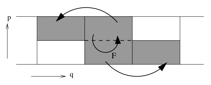
Figure 1: The deterministic model of the walk, an intra-cell dynamics $F$ is followed by horizontally partitioning each cell and shifting the top part left and the bottom part right.

The general class of walks we will consider are deterministic classical dynamical systems whose quantization is given by Eq. (1). The classical phase-space consists of many cells arranged linearly side by side, with intra-cell dynamics say specified by $F$. Each cell as a whole indicates a “site”, and the walk is cell-averaged to give a site to site hopping. Inter-cell dynamics is specified by a binary choice of a cell partition, one being shifted right and other left. The quantization of $F$ is the unitary operator $U$ in Eq. (1), while the choice of the partitions will determine $P_{R}$ and $P_{L}$. The complexity of the coin toss is replaced by the complexity of the classical intra-cell transformation $F$. A schematic illustration of this is shown in Fig. 1, where the partitions have been chosen as equal horizontal splicings. The quantization of the entire map including the shifts is the quantum random walk in Eq. (1). However when we say that, we have made a separation between inter-cell and intra-cell dynamics while both of these occur in the same phase-space and therefore this quantization does not take care of this fact, as noted above.

To illustrate what we mean by the effect of coin dynamics, let us consider the well-studied case of the Hadamard coin. This corresponds to a unitary matrix:

$$U=\frac{1}{\sqrt{2}}\left(\begin{array}[]{cc}1&1\\ 1&-1\end{array}\right),$$ (2)

in the standard basis which we call $\{|\uparrow\rangle,|\downarrow\rangle\}$. The projectors are projectors on the standard basis, $P_{R}=|\uparrow\rangle\langle\uparrow|$ and $P_{L}=|\downarrow\rangle\langle\downarrow|$. The coin dynamics is of course extremely simple, it being a rotation, such that $U^{4}=I$ (since $M=2$, in fact $U^{2}=I$). We generalize this coin by making it higher dimensional and replacing it with the discrete Fourier transform. Thus we take:

$$(U)_{\alpha\beta}=\frac{1}{\sqrt{M}}\exp\left(2\pi i\alpha\beta/M\right);\;\;\;\alpha,\beta=0,\ldots,M-1.$$ (3)

We will use Greek letters to denote states from the cell while Latin letters will refer to the lattice or site states. We note that the above reduces to the Hadamard coin for $M=2$. Also the projectors now generalize to $P_{L}=\sum_{\alpha=0}^{M/2-1}|\alpha\rangle\langle\alpha|$ and $P_{R}=\sum_{\alpha=M/2}^{M-1}|\alpha\rangle\langle\alpha|$. We think of the classical coin dynamics as acting on a unit cell $(q,p)\,\in\,[0,1)\times[0,1)$, while the quantum dynamics is its quantization on this cell after assuming periodic (or quasi-periodic) boundary conditions on $q$ and $p$. Thus $U_{\alpha\beta}$ has the simple interpretation of a quantization of the canonical transformation $F(q,p)=(1-p,q)$ which is a rigid anti-clockwise cell rotation by ninety degrees.

Thus replacing the Hadamard coin with the Fourier transform has a very simple classical limit, a limit that clearly engenders no randomness. This is true even of the walk as a whole, not only for the coin dynamics. The simple coin dynamics engenders a simple walk, in fact the walker does not go very far. Dividing the individual cells into four equal squares, it is easy to see that the walker returns exactly to the beginning point after four time steps. Thus this limit of the Hadamard walk characterized by the size of the Hilbert space $M$ must be such that that $E^{4}(M\rightarrow\infty)=I$, implying a tendency to four-fold spectral degeneracy, and a general reluctance to walk. This is illustrated in Fig. 2, before which we introduce some measures. The probability of starting at cell or site $0$ and arriving at cell $l$ after a time $t$ is

$$p_{l}(t)=\frac{1}{M}\mbox{tr}\left(P_{l}E^{-t}P_{0}E^{t}\right)$$ (4)

where $P_{i}$ is the projection operator on cell $i$. Note that since the cells are linearly arranged, there exists unambiguous quantum projectors such as these. The numbers $p_{l}(t)$ are a discrete probability measure such that $\sum_{l=0}^{L-1}p_{l}(t)=1$. The diffusion in the sites has been usually studied as the second moment of this distribution, the mean squared displacement (m.s.d.):

$$<d^{2}(t)>=\sum_{l=0}^{L-1}p_{l}(t)d_{l}^{2},$$ (5)

where $d_{l}$ is the number of cells from the cell number $0$. This is however partial as it does not properly distinguish generic ballistic motions from simple non-random walks such as plain hopping. Thus the $t^{2}$ law behind the quantum random walks may also be a simple non-random dynamics. As a measure of how many sites are being simultaneously accessed, we need to know how many of the $p_{l}(t)$ at any given time are significant. Thus we may either use an entropy measure $S(t)$ or a participation ratio measure $PR(t)$:

$$S(t)=-\sum_{l=0}^{L-1}p_{l}(t)\log_{L}(p_{l}(t)),\;\,PR(t)=\frac{1}{L\sum_{l=0}^{L-1}p_{l}^{2}(t)}.$$ (6)

The measure $PR(t)$ is the fraction of cells that are occupied at time $t$. We note that for simple hopping while the second moment is quadratic the entropy is zero and the participation ratio is $1/L$.

We also have to point out the following generality. The dimension of the Hilbert space is $ML$, but the uniformity of the coin over the lattice implies that there is translational invariance and hence the lattice-momentum will be conserved and this basis will block diagonalize the unitary operator $E$ into $L$ blocks of size $M$ each. The lattice momentum basis diagonalizes the lattice shift operator $S$:

$$S|k\rangle=e^{2\pi ik/L}|k\rangle.$$ (7)

The vectors $|k\rangle$ are such that $k=0,\ldots,L-1$ and $\langle n|k\rangle=\exp(2\pi ink/L)/\sqrt{L}.$ Then in the lattice-momentum and a cell basis $\{|\alpha\rangle\}$ that could be any orthonormal set, the random walk operator $E$ is block diagonal:

$$\langle k,\alpha|E|k,\beta\rangle=\left\{\begin{array}[]{ll}e^{2\pi ik/L}\langle\alpha|U|\beta\rangle&0\leq\alpha\leq M/2-1\\ e^{-2\pi ik/L}\langle\alpha|U|\beta\rangle&M/2\leq\alpha\leq M-1.\end{array}\right.$$ (8)

We will choose $\{|\alpha\rangle\}$ to be either position or momentum states, thereby partitioning the cells either vertically or horizontally. Thus although the random walk operator $E$ is $LM$ dimensional we can reduce it to $L$, $M$-dimensional operators.

Figure 2: The mean square displacement (m.s.d.), participation ratio and the entropy as a function of time for $M=2$ (solid line), $M=10$ (dotted line) and $M=40$ (dashed line) for the Hadamard-Fourier walk. $L=100$ uniformly.

In Fig. 2, all the three quantities, the m.s.d., the participation ratio and the entropy, are shown for the Hadamard-Fourier walk introduced above and we see that as $M$ increases, indeed the walker gets increasingly lethargic and does not go very far. The oscillatory features seen clearly for $M=10$ and $40$ correspond to period of four and are quantum precursors of the classically exact period-$4$ behaviour. We note that the partitions taken here splice the cells equally vertically rather than horizontally, but this is an inessential feature. Thus the classical limit of the walk with the Hadamard coin via the Fourier coin leads to stunted walks and has its origins in the non-randomness of the classical-coin limit which is a simple rational rotation. This does not mean that the Hadamard Walk in itself has an integrable classical coin limit, as many other coin operators can limit to the Hadamard matrix for $M=2$, other than the Fourier transform. For instance the quantum baker map itself can be a finite $M$ generalization of the Hadamard coin, as pointed out in DD2 . Thus in extreme quantum cases, the notions of integrability and nonintegrability would lose significance. We now turn to cases where the large coin space limit is non-trivial, in fact nonintegrable.

II Nonintegrable coins

We now wish to consider classical dynamics of coins $F(g)$ that depend on a parameter $g$ which can drive it from integrability to chaos. The degree of randomness in the walk will then be controlled by the parameter $g$. In the earlier section we had considered a simple coin which was an integrable example of a rotation. There exist a wide class of models we can choose from, including the so called standard map LL , but we will pick the Harper map, we expect much of what we describe to be independent of such choices.

First, however we briefly mention the exactly solvable case of the multi-baker which has been mentioned earlier. In this case the cell dynamics is the baker transformation:

$$F(q,\,p)=\left\{\begin{array}[]{ll}(2q,\,p/2)&0\leq q<1/2\\ (2q-1,\,(p+1)/2)&1/2\leq q<1.\end{array}\right.$$ (9)

In the infinite chain of such bakers, connected by shifts as described above, if one cell (say cell $1$) is “filled” uniformly (more formally, the initial density is the characteristic function over this cell) the amount of overlap with the other cells will be same as the probability of an unbiased random walker being at that cell, if she were to start from cell $1$. Thus in a very real sense the quantization of such maps are quantum random walks. These have been studied to some extent DanielDorfman but we wish to examine coins that show a range of dynamical behaviour, through a controllable parameter. It may be noted that to the best of our knowledge even classical studies on such systems (“multi-standard”, “multi-Harper”) has not been done and represent rich models from many perspectives in physics.

The Harper map we use subsequently is given by the following transformation:

$$q_{t+1} = q_{t}-\tau\sin(2\pi p_{t})$$

$$p_{t+1} = p_{t}+\tau g\sin(2\pi q_{t+1}),$$ (10)

where $t$ is integer time, and $(q,p)$ is on a unit torus, so modulo one operation is assumed. This is a two-parameter area preserving transformation, and has been studied by many authors for various purposes Harper . This can be derived from the equations of motion of the time-dependent Hamiltonian

$$H=\cos(2\pi p)+g\cos(2\pi q)\sum_{n=-\infty}^{\infty}\delta(2\pi t/\tau-n),$$ (11)

as the map connecting the states just after consecutive kicks. One of the possibilities that seems studied is that for which $g=1$ and the parameter $\tau$ varies. As $\tau/2\pi$ is the time between kicks this alters time-scales in the problem, and therefore we choose to fix $\tau=1$ and consider the Harper map as a function of $g$. Since this phase-space does not seem familiar, we show in fig. 3 some cases, which illustrates a transition to chaos. The routes as $g$ increases seems quite non-trivial as regions of regularity can be created by bifurcations, but by and large the system is almost completely chaotic beyond $g=1$. It may be noted that although we are only displaying the phase-space of $F$, a single cell dynamics, this reflects the phase-space of the complete walker as this will be multiple copies of the same. The somewhat unusual structures visible at $g=0.01$ is because at $\tau=1$ the fixed point(s) at $(q=1/2,p=1/4,3/4)$ is born, and hence this is a marginal situation. We may say in the context of this work that as $g$ increases, the coin becomes increasingly random and the walk it generates will reflect this in ways we want to study.

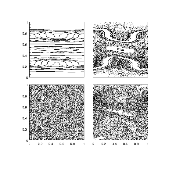
Figure 3: The phase space $(q,p)$ of the classical map for $\tau=1$ and $g=0.01$, $0.05$, $0.1$, and $1$ clockwise from top left.

As is standard the Floquet operator (quantum map) is the quantum propagator:

$$U(g)=\exp(-i\tau g\cos(2\pi\hat{q})/h)\exp(-i\tau\cos(2\pi\hat{p})/h).$$ (12)

With $h=1/M$, we get the quantum version in the basis spanned by the momentum states $|\alpha\rangle$:

$$\langle\alpha|U(g)|\beta\rangle=\exp\left(-i\tau M\cos(2\pi(\beta+\phi)/M)\right)$$

$$\frac{1}{M}\sum_{\gamma=0}^{M-1}\exp\left(-i\tau gM\cos(2\pi(\gamma+\phi)/M)\right)\exp\left(2\pi i(\gamma+\phi)(\beta-\alpha)/M\right).$$ (13)

We have used here the transformation function:

$$\langle\gamma|\alpha\rangle=\frac{1}{\sqrt{M}}\exp\left(2\pi i(\gamma+\phi)(\alpha+\phi)/M\right),$$ (14)

where $|\gamma\rangle$ is a coin position eigenket and $|\alpha\rangle$ is a coin momentum state. The angle $\phi$ refers to boundary conditions on the $M$ coin states and here we have assumed that both position and momentum states acquire a phase of $\exp(2\pi i\phi)$ for a translation of a cell (or $M$ states). We could have assumed two different phases here, but for simplicity we introduce equal phases in both position and momentum states, this phase can be used to break time-reversal (TR) symmetry for the coin dynamics, the effect of which will be felt on the random walker. In the context of the dynamical model we may think of the phase as an Aharanov-Bohm phase that has no effect on the classical dynamics.

We now make use of this unitary coin in the random walk Eq.  (1) and find

$$p_{l}(t)=\frac{1}{M}\sum_{\alpha=0}^{M-1}\sum_{\beta=0}^{M-1}|\langle 0,\alpha|E^{t}|l,\beta\rangle|^{2}.$$ (15)

We then find the entropy, PR, and m.s.d. on the sites as a function of the chaos parameter $g$, coin space dimensionality $M$, and the TR symmetry breaking phase $\phi$. For the rest of the paper we set $\tau=1$ fixing a definite time scale.

In Fig. 4 the various quantities are plotted as a function of time for five representative values of the chaos parameter $g$. We have only shown the first $40$ time steps so that effects of the finite size of the lattice (uniformly $L=100$) is minimized, and is practically independent of this. It is seen that while the m.s.d. is large for the near integrable coin dynamics (small $g$), it is the opposite when considering the PR and entropy of the walk. Both of these quantities are large and are practically the same once chaos has been achieved. This is shown as the near coalescence of the $g=1$ and $g=2$ curves. Thus this figure illustrates the role of deterministic chaos on the quantum walk. We also note the near linear increase in the PR with time in the chaotic cases and the intermediate behavior for mixed coin dynamics. Obviously more detailed study of these features is desirable, but is not pursued here.

Figure 4: The m.s.d., the participation ratio and the entropy as function of time for the multi-Harper walk for various values of the chaos parameter $g$. Uniformly $M=20$ and $L=100$.

Variation of the coin dimensionality $M$ can have a strong impact on the quantum walk and we turn attention in Fig. 5 to this. For a near-integrable case it is seen that the coin-dimensionality does not have a significant impact on the m.s.d. which increases quadratically, however significant deviations are seen for the PR and the entropy. No simple rules are apparently operative, except that for large enough $M$ there is a convergence. For a chaotic case, the m.s.d. is clearly larger for $M=2$ in comparison with larger coins, however PR and entropy wise the larger dimensionality is preferred, although the relationship is not monotonic, for the cases shown $M=8$ seems to produce the most PR and entropy for the times calculated herein.

Figure 5: The m.s.d., the participation ratio and the entropy as function of time for the multi-Harper walk for various values of the coin dimensionality $M$. Shown are one near-integrable (left) and one chaotic (right) cases. The size of the lattice is $L=100$.

Figure 6: The m.s.d., the participation ratio and the entropy as function of time for the multi-Harper walk with $(\phi=0)$ and without time-reversal symmetry $(\phi=0.2)$, for a case that is near-integrable ($g=0.05$) and one that is chaotic ($g=2$). In all cases $M=40$ and $L=100$.

In Fig. 6 is shown the effect of TR symmetry breaking coins. We break the symmetry quite simply by taking a non-zero phase $\phi$, in this case $0.2$. For the nearly integrable/mixed case when $g=0.05$, the TR symmetry breaking has practically no effect while a large effect is seen when there is classical chaos. In the case when the coin dynamics has lost its TR symmetry the walk tends to be slower and produces less entropy. This is because of the additional destructive interference from time reversed paths. The sensitivity to TR symmetry is a general feature of quantum chaos Haake . For instance in the context of information physics and chaos it was recently shown that TR symmetry has a crucial role in determining the distribution of entanglement present in a certain class of many-particle states ArulSubbu . Thus we expect that TR symmetry breaking leads to a decreased diffusion. It must be noted that this is a purely quantum phenomenon, the classical dynamics is completely unaltered by the phases, in fact for initial times the TR symmetric and non-TR symmetric cases go hand-in-hand, a period that agrees with classical laws.

III Discussion

In this paper we have begun the study of a class of deterministic quantum random walkers that generalizes the classical multi-baker maps of Tasaki and Gaspard. These maps show a mixture of regular and chaotic dynamics, and their quantization is in the canonical form of simple random walks. Our main query was what is random in a quantum random walk? In the classical context clearly the source of randomness is the coin-toss and not any process of measurement. Thus we believe that any randomness in quantum random walks must come from using quantum chaotic coins, meaning simply quantized classically chaotic coins. The classical limit in these cases corresponds to the classical limit of the coins, in which case the classical diffusion laws will be obtained. In fact the classical dynamics of such systems as introduced here, namely the multi-Harper maps is itself not studied and represents a potentially rich source of transport models. We have first shown how the generalization of the much studied Hadamard walk is in fact a simple Fourier walk that tends to “go nowhere”, due to its eventual, classical, period-4 behaviour.

We have introduced two natural quantities in studying the quantum walks, the site entropy and the site participation ratio, which measure how well the probability distribution is sampling the sites, rather than only the m.s.d. which tells us how far the walker had gone. In fact we have found that while the m.s.d. is large for nearly regular coins, the entropy and PR are small, indicating the simple nature of the quantum diffusion. On the other hand for chaotic coins the PR and entropy are large and continue to be produced, with the PR increasing linearly in time. We have also shown that TR symmetry breaking suppresses the quantum walk when the coin is chaotic, the most interesting case. We have only aimed at introducing the models and showing primarily a few central numerical results, it is believed that these are of sufficient interest to warrant further study.

- (1) J. Kempe, quant-ph/0303081.
- (2) A. Nayak, A. Vishwanath, quant-ph/0010117, and DIMACS Technical Report 2000-43.
- (3) D. Ornstein, Science 243, 182 (1989).
- (4) A. J. Lichtenberg, and M. A. Lieberman, Regular and Chaotic Dynamics, 2nd ed., Springer-Verlag (New York, 1992).
- (5) N. L. Balazs, and A. Voros, Ann. Phys. (N. Y.) 190 (1989) 1; M. Saraceno, Ann. Phys. (N.Y.) 199, 37, (1990).
- (6) D. K. Wojcik, J. R. Dorfman, Phys. Rev. E 66, 036110 (2002); quant-ph/0209036.
- (7) D. K. Wojcik, J. R. Dorfman, quant-ph/0212036.
- (8) P. Gaspard, J. Stat. Phys. 68, 673 (1992).
- (9) S. Tasaki, P. Gaspard, J. Stat. Phys. 101, 125 (1995).
- (10) A. Lakshminarayan, N. L. Balazs, J. Stat. Phys. 77, 311 (1994).
- (11) R. Artuso, G. Casati, F. Borgonovi, L. Rebuzzini, Int. J. Mo d. Phys. B 8 207 (1994); P. Leboeuf, J. Kurchan, M. Feingold and D. P. Arovas, Phys . Rev. Lett. 65 3076 (1990); R. Lima and D. Shepelyansky, Phys. Rev. Lett. 67, 1377 (1991).
- (12) A. Lakshminarayan, V. Subrahmanyam, Phys. Rev. A. To Appear (May 2003). quant-ph/0212049.
- (13) F. Haake, Quantum Signature of Chaos 2nd Ed. Springer-Verlag (Berlin, 2001).