Measurement-induced decoherence and Gaussian smoothing of the Wigner distribution function

Abstract

We study the problem of measurement-induced decoherence using the phase-space approach employing the Gaussian-smoothed Wigner distribution function. Our investigation is based on the notion that measurement-induced decoherence is represented by the transition from the Wigner distribution to the Gaussian-smoothed Wigner distribution with the widths of the smoothing function identified as measurement errors. We also compare the smoothed Wigner distribution with the corresponding distribution resulting from the classical analysis. The distributions we computed are the phase-space distributions for simple one-dimensional dynamical systems such as a particle in a square-well potential and a particle moving under the influence of a step potential, and the time-frequency distributions for high-harmonic radiation emitted from an atom irradiated by short, intense laser pulses.

and

1 Introduction

Quantum phase-space distribution functions [1, 2] offer an alternative means of formulating quantum mechanics to the standard wave mechanics formulation. Some of the properties that these functions possess, however, make it difficult to associate them with a direct probabilistic interpretation. The Wigner distribution function [3], for example, can take on negative values, while the Husimi distribution function [4], although nonnegative, does not yield the correct marginal distributions. These functions are therefore usually regarded as a mathematical tool used to describe the quantum behavior of the system being considered and are thus referred to as the quasiprobability distribution functions.
There, however, have been continued theoretical investigations [5, 6, 7] on the possibility of the physical significance of the Husimi distribution function and more generally of the nonnegative smoothed Wigner distribution function, ever since Arthurs and Kelly [5] showed that the Husimi distribution is a proper probability distribution associated with a particular model of simultaneous measurements of position and momentum. An operational definition of a probability distribution can be given [6] that explicitly takes into account the action of the measurement device modeled as a “filter”. The analysis shows that the phase-space distribution connected to a realistic simultaneous measurement of position and momentum can be expressed as a convolution of the Wigner function of the system being detected and the Wigner function of the filter state. If the Wigner function of the filter state is given by a minimum uncertainty Gaussian function, which is the case for an ideal simultaneous measurement with the maximal accuracy allowed by the Heisenberg uncertainty principle, the distribution can be identified as the Husimi distribution. A generalization to the case of a measurement with less accuracy leads immediately to an identification of the nonnegative smoothed Wigner distribution as a distribution connected to a realistic measurement.
It is then clear that, in the phase-space approach, the act of a measurement is conveniently modeled by Gaussian smoothing, with the widths of the smoothing function identified as measurement errors. The phase-space approach based on the smoothed Wigner distribution function thus provides a convenient framework in which to study any changes that occur in the phase-space distribution of a system as a result of a measurement.
In this paper we aim to investigate effects of a measurement on the phase-space distribution of a system using the phase-space description based on the smoothed Wigner distribution function [8]. We consider some simple one-dimensional systems—a particle in a square-well potential, a particle moving under the influence of a step potential, and a one-dimensional model atom irradiated by high-power laser pulses emitting high-harmonic radiation—and compute their Wigner and smoothed Wigner distribution functions. The pure quantum distribution of the systems unaffected by a measurement is represented by contour curves of the Wigner distribution functions, whereas the “coarse-grained” distribution, i.e., the distribution “contaminated” by a measurement is displayed by contour curves of the smoothed Wigner distribution functions. It may be expected that delicate quantum features are obscured more strongly by a measurement with larger measurement errors. Such effects of a measurement, which may be referred to as measurement-induced decoherence, can be studied by observing changes in the contour curves of the smoothed Wigner distribution functions, as the widths of the smoothing Gaussian function are increased. We also compare the contour curves of the smoothed Wigner distributions we computed with the corresponding contour curves resulting from the classical analysis. This should yield information on what quantum features survive measurement-induced decoherence.
In Section 2 we briefly describe the Wigner and smoothed Wigner distribution functions and discuss their physical significance in relation to a measurement. In Section 3 we choose, as our examples of simple dynamical systems, a particle in an infinite square-well potential and a particle subjected to a step potential and compute their contour curves of the Wigner and smoothed Wigner distribution functions. These contour curves form the basis of our discussion of measurement-induced decoherence. Another example we take for our study is a one-dimensional model atom irradiated by high-power laser pulses, which is described in Section 4. The time-frequency Wigner and smoothed Wigner distributions are computed for high-harmonic radiation emitted from the model atom, and the effect of a measurement on the time-frequency distribution is discussed. Finally a discussion is given in Section 5.

2 Wigner and smoothed Wigner distribution functions

The Wigner distribution function [3] is defined by

$$W(q,p)=\frac{1}{\pi\hbar}\int dxe^{-2ipx/\hbar}\Psi^{\ast}(q-x)\Psi(q+x),$$ (2.1)

where $q$ and $p$ are the coordinate and the momentum of the system being considered and $\Psi$ is the wave function. In our study of one-dimensional dynamical systems, we restrict our attention to the simple case when the system is in its energy eigenstate. The wave function $\Psi$ and the Wigner distribution function $W$ is then independent of time. The Gaussian-smoothed Wigner distribution function [8] is given by

$$G(q,p)=\frac{1}{2\pi\sigma_{q}\sigma_{p}}\int dq^{\prime}\int dp^{\prime}e^{-\frac{(q^{\prime}-q)^{2}}{2\sigma_{q}^{2}}}e^{-\frac{(p^{\prime}-p)^{2}}{2\sigma_{p}^{2}}}W(q^{\prime},p^{\prime}).$$ (2.2)

When the smoothing Gaussian function is a minimum uncertainty wave packet, i.e., when $\sigma_{q}\sigma_{p}=\frac{\hbar}{2}$, $G$ can be identified as the Husimi distribution function,

$$H(q,p)=\frac{1}{2\pi\hbar}\sqrt{\frac{\kappa}{\pi\hbar}}\left|\int dxe^{-\kappa(x-q)^{2}/2\hbar}e^{-ipx/\hbar}\Psi(x)\right|^{2},$$ (2.3)

where the parameter $\kappa$ defined as $\kappa=\frac{\hbar}{2\sigma_{q}^{2}}=\frac{2\sigma_{p}^{2}}{\hbar}$ has the dimension of $mass/time$. If $G$ is to represent a probability distribution corresponding to a simultaneous measurement of $q$ and $p$, the widths should satisfy the inequality $\sigma_{q}\sigma_{p}\geq\frac{\hbar}{2}$, where $\sigma_{q}$ and $\sigma_{p}$, respectively, can be identified as measurement errors in $q$ and $p$ of the detection apparatus. For general mathematical treatments, however, one may also include the unphysical regime $\sigma_{q}\sigma_{p}<\frac{\hbar}{2}$ in the analysis . In particular, in the limit $\sigma_{q}\to 0$ and $\sigma_{p}\to 0$, $G(q,p)$ approaches the Wigner function $W(q,p)$.
In general the Wigner function can be defined in space of any pair of conjugate variables. In particular, in studies of signal processing, the Wigner function in the time-frequency space, $W(t,\omega)$, plays an important role [9]. The main tool for our time-frequency analysis of high-harmonic radiation generated by an atom irradiated by laser pulses, which is described in Section 4, is the Wigner time-frequency distribution function of the dipole acceleration

$$W(t,\omega)=\frac{1}{\pi}\int_{-\infty}^{\infty}d\tau e^{-2i\omega\tau}\ddot{d}^{\ast}(t-\tau)\ddot{d}(t+\tau),$$ (2.4)

where the dipole acceleration $\ddot{d}(t)$ is given by

$$\ddot{d}(t)=\frac{d^{2}}{dt^{2}}d(t)=\langle\Psi(t)\left|\ddot{x}\right|\Psi(t)\rangle.$$ (2.5)

In Eq. (2.5), $\Psi(t)$ represents the wave function of the electron in the atom and $x$ is the position of the electron. The Gaussian-smoothed Wigner distribution function in time-frequency space is given by

$$G(t,\omega)=\frac{1}{2\pi\sigma_{t}\sigma_{\omega}}\int dt^{\prime}\int d\omega^{\prime}e^{-\frac{(t^{\prime}-t)^{2}}{2\sigma_{t}^{2}}}e^{-\frac{(\omega^{\prime}-\omega)^{2}}{2\sigma_{\omega}^{2}}}W(t^{\prime},\omega^{\prime}).$$ (2.6)

When the widths $\sigma_{t}$ and $\sigma_{\omega}$ satisfy $\sigma_{t}\sigma_{\omega}=\frac{1}{2}$, $G$ becomes the Husimi time-frequency distribution function

$$H(t,\omega)=\frac{1}{2\pi}\sqrt{\frac{\kappa}{\pi}}\left|\int d\tau e^{-\kappa(\tau-t)^{2}/2}e^{-i\omega\tau}\ddot{d}(\tau)\right|^{2},$$ (2.7)

where the parameter $\kappa$ given by $\kappa=\frac{1}{2\sigma_{t}^{2}}=2\sigma_{\omega}^{2}$ has now the dimension of $(time)^{-2}$.
Since the measurement errors satisfying the inequality $\sigma_{q}\sigma_{p}\geq\frac{\hbar}{2}$ (or $\sigma_{t}\sigma_{\omega}\geq\frac{1}{2}$) belong to the physical regime, the contour curves of $G$ associated with the smoothing Gaussian function satisfying this inequality can in principle be observed. Perhaps the most straightforward way of constructing such contour curves from measurements is to make a large number of simultaneous measurements of position and momentum (or time and frequency) upon identically prepared systems. Each measurement should be performed with the same measurement errors $\sigma_{q}$ and $\sigma_{p}$ (or $\sigma_{t}$ and $\sigma_{\omega}$). Each measurement should also be performed on a given system no more than once, because the measurement disturbs the system and its phase-space distribution. From the results of such measurements one can determine the phase-space distribution (or the time-frequency distribution) for the system under consideration. The contour curves of the smoothed Wigner distribution function associated with the widths $\sigma_{q}$ and $\sigma_{p}$ (or $\sigma_{t}$ and $\sigma_{\omega}$) of the smoothing Gaussian function are then obtained by connecting the phase-space points (or the time-frequency points) having the same phase-space probability (or the same time-frequency space probability).
Our main concern here is the effects of a measurement on quantum properties of a system. Information on such effects can be directly obtained by comparing contour curves of the Wigner distribution function and those of various smoothed Wigner distribution functions associated with different values of $\sigma_{q}$ and $\sigma_{p}$ (or $\sigma_{t}$ and $\sigma_{\omega}$). In the next two sections we present results for our computation of the contour curves in phase space for two simple one-dimensional dynamical systems and in time-frequency space for high-harmonic radiation emitted by an atom irradiated by laser pulses.

3 One-dimensional dynamical systems in a stationary state

In this section we present results of our computation of contour curves of the Wigner and smoothed Wigner distribution functions for two simple systems in a stationary state; a particle in a symmetric infinite square-well potential and a particle moving under the influence of a step potential. For stationary systems it is possible to obtain contour plots of the Wigner distribution function directly by solving a pair of time-independent equations of motion satisfied by the Wigner function [10]. One can also derive a pair of time-independent equations of motion for the smoothed Wigner distribution function and can thus obtain its contour plots from the solutions of these equations. In the present work, however, we have chosen to numerically integrate the Wigner distribution function according to Eq. (2.2) in order to obtain contour curves of the smoothed Wigner distribution function, because an analytical form for the Wigner distribution function is known for each of the two systems being considered here.

3.1 Particle in a square well

We consider a particle in a symmetric infinite square-well potential

$$V(q)=\begin{cases}0,&\text{if $-a\leq q\leq a$,}\\ \infty,&\text{if $q<-a$, or $q>a$}.\end{cases}$$ (3.1)

An analytic form for the Wigner distribution function is known for this system in its eigenstate [11]. For all our computation we take the mass of the particle to be 1 and the width of the well to be 20 in an arbitrary unit system in which $\hbar=1$.
Shown in Figs. 1(a) and 1(b) are contour plots of the Wigner distribution function and the smoothed Wigner distribution function, respectively, for the particle in its ground state. The smoothing parameters for Fig. 1(b) are chosen to be $\sigma_{q}=3.62$ and $\sigma_{p}=0.157$ ($\sigma_{q}\sigma_{p}=0.57>\frac{\hbar}{2}$). Comparing Figs. 1(a) and 1(b), we see that the smoothed Wigner distribution function has a simpler structure than the nonsmoothed Wigner distribution function. This reflects the effect of measurement-induced decoherence. The most conspicuous quantum structure which is exhibited in Fig. 1(a) but is not revealed when observed with $\sigma_{q}=3.62$ and $\sigma_{p}=0.157$ is closed orbits off the origin called “islands”. Two pairs of the islands are shown in Fig. 1(a). Close inspection of the contour plot of the Wigner distribution function, however, reveals many such islands, although not shown in the figure. We note that a purely classical dynamical consideration would indicate that the contour lines of the classical probability follow classical trajectories. Thus, for the present case of a particle in a square-well potential, classical contour lines would consist of a set of pairs of straight horizontal lines in the region $-a\leq q\leq a$. It is interesting to note that the contour curves of the smoothed Wigner function, Fig. 1(b), are not straight lines, which indicate that some quantum characteristics still survive Gaussian smoothing. The quantum dynamical property represented by curved contour curves may be referred to as nonlocality, because these curves lead one to interpret that the particle changes its momentum even before it actually hits the potential wall. (For classical dynamical interpretation of Wigner contour curves and problems arising from it, see [11] and [12].) This quantum behavior (curved contour curves) lies within the limits of observation because Fig. 1(b) belongs to the physical regime ($\sigma_{q}\sigma_{p}\geq\frac{\hbar}{2}$).
Figs. 2(a)-2(d) show contour curves for the same particle in its fifth eigenstate [13]. The contour plot of the Wigner distribution function shown in Fig. 2(a) indicates that there are five maxima along the $q$ axis arising from the five-peak standing wave structure of the eigenfunction and two maxima along the $p$ axis corresponding to the momenta to the right and left, respectively, of the classical particle of the same energy. Characteristic quantum features such as curved contour lines and the formation of islands are even more evident here. Figs. 2(b) and 2(c) are contour plots of the Husimi distribution function ($\sigma_{q}\sigma_{p}=\frac{\hbar}{2}$) with $\sigma_{q}=0.637$, $\sigma_{p}=0.785$, and with $\sigma_{q}=5.70$, $\sigma_{p}=0.0877$, respectively. One sees that a choice of a large $\sigma_{q}$ ($\sigma_{p}$) results in strong smoothing along the $q$ ($p$) axis. These two figures represent the quantum phase-space distribution connected to ideal simultaneous measurements with different degrees of the position vs. momentum uncertainties. The fact that Husimi curves are different for a different choice of $\sigma_{q}$ or $\sigma_{p}$ means physically that the quantum distribution looks different depending on how one observes it. It should be noted that the curves of Figs. 2(b) and 2(c), although simpler in structure than the curves of Fig. 2(a) due to measurement-induced decoherence, still exhibit strong quantum behavior such as the islands even though they belong to the physical regime. This can be understood if we note that the uncertainties $\Delta_{q}\equiv\sqrt{\langle q^{2}\rangle-\langle q\rangle^{2}}$ and $\Delta_{p}\equiv\sqrt{\langle p^{2}\rangle-\langle p\rangle^{2}}$ associated with the fifth eigenstate are given by $\Delta_{q}=5.70$ and $\Delta_{p}=0.785$ ($\Delta_{q}\Delta_{p}=4.48$). The widths $\sigma_{q}$ and $\sigma_{p}$ of the smoothing Gaussian function used for Figs. 2(b) and 2(c) are less than the uncertainties $\Delta_{q}$ and $\Delta_{p}$ inherent in the fifth eigenstate, and therefore the probabilistic nature of the quantum eigenstate is expected to be displayed by the corresponding contour curves. Fig. 2(d) shows contour plots for the case $\sigma_{q}=\Delta_{q}$ and $\sigma_{p}=\Delta_{p}$. One sees now that the islands, a clear indication of a strong quantum feature, have disappeared. Note, however, that the nonlocal nature (i.e., curved contour curves) is still indicated by the contour curves of Fig. 2(d), as these curves deviate from the corresponding classical trajectories, i.e., straight horizontal lines.

3.2 Particle incident on a potential step

As a second example we consider a particle of fixed energy $E$ moving under the influence of a step potential

$$V(q)=\begin{cases}0,&\text{if $q<0$,}\\ V_{0},&\text{if $q\geq 0$.}\end{cases}$$ (3.2)

The wave function and the Wigner distribution function for this particle have been given earlier [11]. The parameter values we have chosen for our computation are $m=1$, $V_{0}=1$, $E=0.5$ in an arbitrary unit system in which $\hbar=1$. Since the particle energy $E$ is one half the potential step $V_{0}$, the wave function decreases exponentially with respect to $q$ in the region $q\geq 0$.
Fig. 3(a) shows a contour plot of the Wigner distribution function for the particle. In addition to the quantum features such as curved contour lines and the islands that are already exhibited by the Wigner curves of the particle in a square-well potential, we see that some curves exhibit tunneling into the potential step.
In Figs. 3(b) and 3(c) we show contour plots of the Husimi distribution function for the cases $\sigma_{q}=0.5$, $\sigma_{p}=1$ and $\sigma_{q}=1.58$, $\sigma_{p}=0.316$, respectively. Strong quantum features such as nonlocality, islands and tunneling are still clearly shown, although the curves belong to the physical regime. This can be understood by recalling that, for the particle of energy $E=0.5$ being considered here, $\Delta_{q}\to\infty$ (since the particle is extended in the entire half space $q<0$) and $\Delta_{p}=\sqrt{2mE}=1$, and the widths $\sigma_{q}$ and $\sigma_{p}$ chosen for Figs. 3(b) and 3(c) are still sufficiently small that the quantum nature of the eigenfunction survives.
Finally in Fig. 3(d) we show a contour plot of the smoothed Wigner distribution function with $\sigma_{q}=2.236$, $\sigma_{p}=1$. Although the islands have disappeared now, the curves still exhibit nonlocality and tunneling. The curves are not quite the same as the classical trajectories which consist of a set of pairs of straight lines in the region $q<0$ for $E<V_{0}$.

4 High-harmonic radiation generated by a one-dimensional atom irradiated by laser pulses

The phenomenon of high-harmonic generation in atomic gases irradiated by high-power laser pulses has been investigated intensively in the past both theoretically and experimentally [14]. A typical emission spectrum observed experimentally shows a broad plateau extending to high-order harmonics accompanied with a fast cutoff. The mechanism by which high-order harmonics are generated is now well understood. In particular, the simple classical three-step model [15] has been quite useful in providing the conceptual understanding of this phenomenon.
In this work we focus on the time-frequency distribution of the emitted radiation, i.e., on the relationship between the time of emission and the frequency of emitted radiation. Since the temporal variation of the emitted signal can be represented by the dipole acceleration [16], the pure quantum-mechanical time-frequency distribution of the emitted radiation is described by the Wigner time-frequency distribution of the dipole acceleration as defined in Eq. (2.4) [17]. Our main interest lies in the effect of measurement on this Wigner time-frequency distribution. In this particular case, the measurement should consist of the simultaneous measurement of time and frequency. One needs to perform a large number of such measurement upon a large number of identically prepared samples (atomic gases irradiated by laser pulses). The time-frequency distribution associated with the measurements with the uncertainties $\sigma_{t}$ and $\sigma_{\omega}$ is given by the Gaussian-smoothed Wigner distribution $G(t,\omega)$ of Eq. (2.6). We also compare this smoothed Wigner distribution with the corresponding distribution resulting from classical analysis.
In subsection 4.1 we give a brief description of the system. In subsection 4.2 we then find the classical time-frequency distribution based on the three-step model. The main part of this section is subsection 4.3 in which quantum time-frequency distribution, both Wigner and smoothed Wigner, are presented.

4.1 System

The system under consideration is a one-dimensional model atom irradiated by laser pulses. The wave function of the electron in the atom evolves with time according to the time-dependent Schrödinger equation which reads in atomic units

$$i\frac{\partial}{\partial t}|\Psi(t)\rangle=\left[\frac{p^{2}}{2}+V(x)-xE(t)\right]|\Psi(t)\rangle,$$ (4.1)

where the atomic potential $V(x)$ is modeled upon a soft-core potential of the form

$$V(x)=-\frac{1}{\sqrt{\beta^{2}+x^{2}}}.$$ (4.2)

We set $\beta\cong 0.67$ a.u. in order for the system to have a ground-state energy equivalent to the binding energy $I_{p}$ of Ne. The laser pulse incident on the atom is assumed to be a Gaussian pulse with the electric field $E(t)$ given by

$$E(t)=E_{0}\exp\left[-2\ln 2\frac{t^{2}}{(\Delta t)^{2}}\right]\cos(\omega_{L}t).$$ (4.3)

In our calculations, we take the center frequency of the pulse, $\omega_{L}=800$ nm, the full width at half maximum of the laser pulse, $\Delta t=160$ fs, and the peak intensity $3\times 10^{14}$ $\rm W/cm^{2}$.

4.2 Classical analysis

Here we consider the question of when each harmonic is emitted. If one uses classical analysis based on the three-step model [15], it is straightforward to obtain the relation between the time of emission and the frequency of emitted radiation. After tunneling through the Coulomb barrier, different electrons in atoms at different locations in general see the laser field at different phases and therefore follow different classical trajectories. Consequently, different electrons return to their nuclei at different times with different kinetic energies. Let us say that the $i$th electron returns to its nucleus at time $t_{i}$ with kinetic energy $K_{i}=\frac{1}{2}mv_{i}^{2}$. When this electron recombines with the nucleus, the radiation of frequency $\omega_{i}$ given by $\hbar\omega_{i}=I_{p}+K_{i}$ is emitted. Collecting $\omega_{i}$ and $t_{i}$ for all different electrons, one has the answer to the question of when the radiation of a given frequency is emitted. The solid curves in Fig. 4 shows the result of such classical calculations. The curves exhibit the characteristic $\Lambda$ structure, which indicates that, within one-half optical cycle of the laser field, there exist two different classical trajectories, called “short” and “long” paths, with two different return times that lead to an emission of radiation of a given frequency [18]. The open circles in Fig. 4 represent contributions from multiple recollisions. There is a possibility that recombination does not occur when the electron returns to its nucleus. One thus needs to consider the cases when the electron recombines with the nucleus at the $n$th ($n\geq 2$) encounter with the nucleus. These open circles together with the solid curves of the $\Lambda$ structure comprise the classical time-frequency distribution obtained using the three-step model.

4.3 Quantum-mechanical analysis

We now turn to a quantum time-frequency distribution of the emitted radiation [17]. For our computation of the Wigner distribution of Eq. (2.4), we first solve the time dependent Schrödinger equation, Eq. (4.1), using the Crank-Nicolson method. Once $\Psi(t)$ is known, the dipole acceleration $\ddot{d}(t)$ can be calculated using Eq. (2.5) and then the Wigner time-frequency distribution $W(t,\omega)$ can be obtained using Eq. (2.4). The Gaussian-smoothed Wigner distribution $G(t,\omega)$ can then be obtained using Eq. (2.6). In particular, the Husimi time-frequency distribution can be computed relatively easily by using Eq. (2.7).
The Wigner time-frequency distribution $W(t,\omega)$ we computed shows a very complicated structure, and it is difficult to extract physical meaning out of it. We therefore choose not to show it here and just to mention that it consists of a large number of small islands, a clear indication that strong quantum behavior is exhibited by the time-frequency distribution.
In Figs. 5(a)-5(c), we show Gaussian-smoothed Wigner time-frequency distributions we computed. The widths of the smoothing Gaussian function are $\sigma_{t}=2.236$ and $\sigma_{\omega}=0.224$ for Fig. 5(a). Since $\sigma_{t}\sigma_{\omega}=\frac{1}{2}$, Fig 5(a) is the Husimi time-frequency distribution. For Figs. 5(b) and 5(c), we have $\sigma_{t}=2.236$, $\sigma_{\omega}=0.448$, and $\sigma_{t}=4.472$, $\sigma_{\omega}=0.224$, respectively. We note that the overall shape of the smoothed Wigner distributions suggests the $\Lambda$ structure of the classical distribution of Fig. 4. The similarity, however, is only qualitative, because the smoothed Wigner distributions have many detailed structures (many islands) absent in the classical distribution. We mention, however, that the smoothed distributions of Figs. 5(a)-5(c) are much simpler than the nonsmoothed Wigner distribution not shown. We see from Figs. 5(a)-5(c) that the distribution in the low-order region takes on the maximum value at times 0.5, 1.0, 1.5, 2.0, etc, i.e. at times at which the laser field amplitude takes on the maximum or minimum value. The $\Lambda$-like structure in the midplateau region shown in Figs. 5(a)-5(c) indicates that photons in the plateau region are emitted mainly at two different times within one-half cycle of the laser field, in agreement with the classical analysis based on Fig. 4. The separation between these two times decreases and eventually vanishes as the harmonic order is increased toward the cutoff. In the cutoff region, therefore, photons are emitted once within one-half cycle. Figs. 5(a)-5(c) show that the distribution in the cutoff region is maximum at times 0.7, 1.2, 1.7, 2.2, etc, indicating that photons in the cutoff region are emitted at times just before the laser amplitude vanishes.

5 Discussion

In this paper we have studied effects of a measurement on the phase-space (time-frequency) distribution using the approach based on the smoothed Wigner distribution function. The physical significance of the phase-space (time-frequency) contour curves differs depending on the widths $\sigma_{q}$ and $\sigma_{p}$ ($\sigma_{t}$ and $\sigma_{\omega}$) of the smoothed Wigner distribution function used. While the contour curves of the nonsmoothed Wigner distribution function with $\sigma_{q}\to 0$ and $\sigma_{p}\to 0$ ($\sigma_{t}\to 0$ and $\sigma_{\omega}\to 0$) represent the unobservable pure quantum distribution, the Husimi curves with $\sigma_{q}\sigma_{p}=\frac{\hbar}{2}$ ($\sigma_{t}\sigma_{\omega}=\frac{1}{2}$) represent the quantum distribution observed in ideal simultaneous measurements with the maximal accuracy allowed by the Heisenberg uncertainty principle. In general, contour curves in the physical regime corresponding to $\sigma_{q}\sigma_{p}\geq\frac{\hbar}{2}$ ($\sigma_{t}\sigma_{\omega}\geq\frac{1}{2}$) represent the quantum distribution associated with a coarse-grained observation caused by measurement errors. We have seen that quantum features such as the islands tend to disappear and the resulting quantum distribution becomes simpler in structure, as the measurement errors are increased. In general, however, the smoothed Wigner distributions associated with relatively large measurement errors have more structures than the corresponding classical distributions.
In conclusion we have shown, with simple one-dimensional model systems as examples, that the phase-space formulation based on the smoothed Wigner distribution function provides a very natural framework in which to study how the quantum phase-space distribution is affected by a measurement.

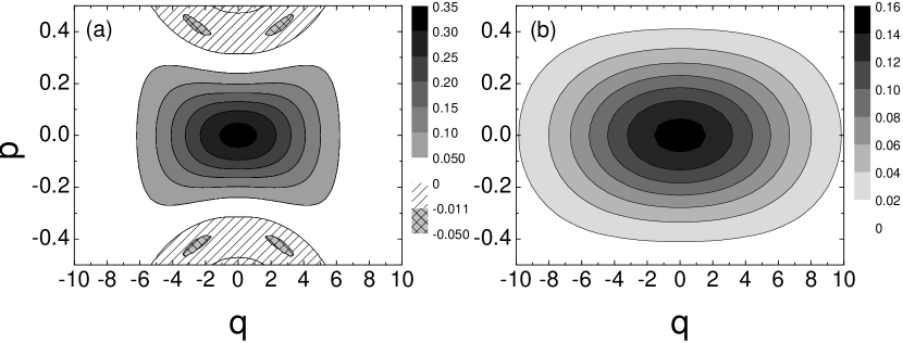
Figure 1:

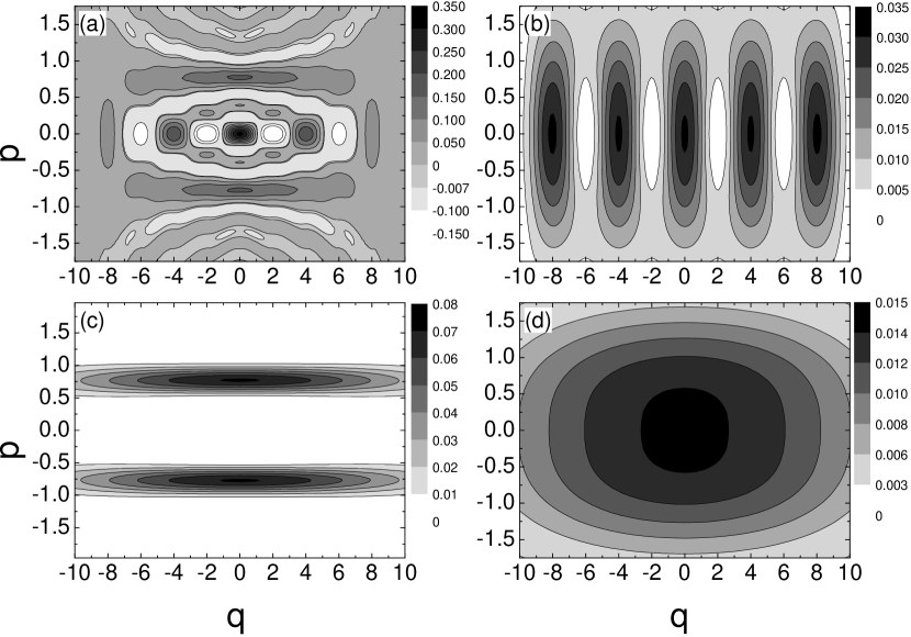
Figure 2:

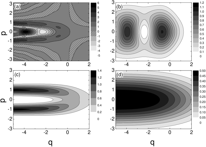
Figure 3:

Figure 4:

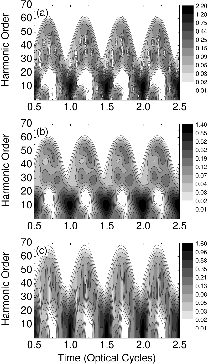
Figure 5:

References

- [1] M. Hillery, R. F. O’Connel, M. O. Scully, and E. P. Wigner, Phys. Rep. 106, 121 (1984).
- [2] H. W. Lee, Phys. Rep. 259, 147 (1995).
- [3] E. Wigner, Phys. Rev. 40, 749 (1932).
- [4] K. Husimi, Prog. Phys. Math. Soc. Japan 22, 264 (1940).
- [5] E. Arthurs and J. L. Kelly, Jr., Bell Syst. Tech. J. 44, 725 (1965).
- [6] K. Wodkiewicz, Phys. Rev. Lett. 52, 1064 (1984).
-
[7]
E. Prugovecki,
Ann. Phys. 110, 102 (1978);
S. T. Ali and E. Prugovecki, J. Math. Phys. 18, 219 (1977);
K. Takahashi and N. Saito, Phys. Rev. Lett. 55, 645 (1985);
S. L. Braunstein, C. M. Caves, and G. J. Milburn, Phys. Rev. A 43, 1153 (1991);
S. Stenholm, Ann. Phys. 218, 233 (1992);
D. M. Appleby, J. Phys. A : Math. Gen. 31, 6419 (1998). -
[8]
N. D. Cartwright,
Physica 83A, 210 (1976);
R. F. O’Connel and E. P. Wigner, Phys. Lett. 85A, 121 (1981);
A. Jannussis, N. Patargias, A. Leodaris, P. Filippakis, T. Filippakis, A. Streclas, and V. Papatheou, Lett. Nuovo Cimento 34, 553 (1982);
D. Lalovic, D. M. Davidovic, and N. Bijedic, Physica A 184, 231 (1992). - [9] See, for example, L. Cohen, Proc. IEEE 77, 941 (1989).
-
[10]
D. B. Fairlie,
Proc. Camb. Phil. Soc. 60, 581 (1964);
W. Kundt, Z. Naturforsch. 22a, 1333 (1967);
T. Curtright, D. Fairlie, and C. Zachos, Phys. Rev. D 58, 025002 (1998);
M. Hug, C. Menke, and W. P. Schleich, J. Phys. A 31, L217 (1998). - [11] H. W. Lee and M. O. Scully, Found. Phys. 13, 61 (1983).
-
[12]
H. W. Lee,
Found. Phys. 22, 995 (1992);
H. W. Lee, Phys. Lett. A, 146, 287 (1990);
R. Sala, S. Brouard, and J. G. Muga, J. Chem. Phys. 99, 2708 (1993);
K. L. Jensen and F. A. Buot, Appl. Phys. Lett. 55, 669 (1989);
N. E. Henriksen, G. D. Billing, and F. Y. Hansen, Chem. Phys. Lett. 149, 397 (1988);
G. W. Bund, S. S. Mizrahi, and M. C. Tijero, Phys. Rev. A 53, 1191 (1996);
T. Curtright and C. Zachos, J. Phys. A 32, 771 (1999);
M. Hug and G. J. Milburn, Phys. Rev. A 63, 023413 (2001);
A. L. Rivera, N. M. Atakishiyev, S. M. Chumakov, and K. B. Wolf, Phys. Rev. A 55, 876 (1997);
B. Segev, Phys. Rev. A 63, 052114 (2001). -
[13]
M. A. M. de Aguiar and A. M. O. de Almeida,
J. Phys. A 23, L1025 (1990);
H. W. Lee, Phys. Rev. A 50, 2746 (1994). - [14] For a review, see, e.g., M. Protopapas, C. H. Keitel, and P. L. Knight, Rep. Prog. Phys. 60, 389 (1997).
-
[15]
J. L. Krause, K. J. Schafer, and K. C. Kulander,
Phys. Rev. Lett. 68, 3535 (1992);
K. J. Schafer, B. Yang, L. F. DiMauro, and K. C. Kulander, Phys. Rev. Lett. 70, 1599 (1993);
P. B. Corkum, Phys. Rev. Lett. 71, 1994 (1993). - [16] J. B. Watson, A. Sanpera, and K. Burnett, Phys. Rev. A 51, 1458 (1995).
- [17] J. H. Kim, D. G. Lee, H. J. Shin, and C. H. Nam, Phys. Rev. A 63, 063403 (2001).
-
[18]
P. Salières, A. L’Huillier, and M.
Lewenstein, Phys. Rev. Lett. 74, 3776 (1995);
M. Lewenstein, P. Salières, and A. L’Huillier, Phys. Rev. A 52, 4747 (1995);
Ph. Balcou, A. S. Dederichs, M. B. Gaarde, and A. L’Huillier, J. Phys. B 32, 2973 (1999);
M. Bellini, C. Lynga, A. Tozzi, M. B. Gaarde, T. W. Hänsch, A. L’Huillier, and C. G. Wahlström, Phys. Rev. Lett. 81, 297 (1998);
D. G. Lee, H. J. Shin, Y. H. Cha, K. H. Hong, J. H. Kim, and C. H. Nam, Phys. Rev. A 63, 021801(R) (2001).
Figure Captions
Figure 1. Contour plots for a particle in a symmetric infinite square-well potential in its ground state. The mass of the particle is 1 and the width of the potential well is 20 in an arbitrary unit system in which . (a) Wigner function, (b) smoothed Wigner function with and .
Figure 2. Same as Figure 1 except that the particle is in its fifth eigenstate. (a) Wigner function, (b) Husimi function with , , (c) Husimi function with , , (d) smoothed Wigner function with , .
Figure 3. Contour plots for a particle moving under the influence of a step potential. The mass and energy of the particle are 1 and 0.5, respectively, and the value of the potential is 0 for and 1 for , in an arbitrary unit system in which . (a) Wigner function, (b) Husimi function with , , (c) Husimi function with , , (d) smoothed Wigner function with , .
Figure 4. Classical time-frequency distribution for high-harmonic radiation. The solid curves represent contributions from the short and long paths, and the open circles represent contributions from multiple recollisions.
Figure 5. Contour plots for high-harmonic radiation. (a) Husimi function with , , (b) smoothed Wigner function with , , (c) smoothed Wigner function with , .