Quantum Physics of Simple Optical Instruments

Abstract

Simple optical instruments are linear optical networks where the incident light modes are turned into equal numbers of outgoing modes by linear transformations. For example, such instruments are beam splitters, multiports, interferometers, fibre couplers, polarizers, gravitational lenses, parametric amplifiers, phase-conjugating mirrors and also black holes. The article develops the quantum theory of simple optical instruments and applies the theory to a few characteristic situations, to the splitting and interference of photons and to the manifestation of Einstein-Podolsky-Rosen correlations in parametric downconversion. How to model irreversible devices such as absorbers and amplifiers is also shown. Finally, the article develops the theory of Hawking radiation for a simple optical black hole. The paper is intended as a primer, as a nearly self-consistent tutorial. The reader should be familiar with basic quantum mechanics and statistics, and perhaps with optics and some elementary field theory. The quantum theory of light in dielectrics serves as the starting point and, in the concluding section, as a guide to understand quantum black holes.

1 Introduction

Consider a semi-transparent mirror, the glass of your window, for example. The mirror partially reflects light and is partially transparent. If the material of the mirror is not absorptive the incident light is exactly split into the reflected and the transmitted component. Now, light consists of photons, of indivisible light particles. How does this beam splitter act on individual photons [32, 146]? How are photons split? Or, in another experiment [71], suppose you take a semi-silvered mirror with 50:50 transmission-reflection ratio. You let exactly one photon propagate towards the frontside of the mirror and you send another single photon towards the backside, and let them interfere. The interference between two light beams depends on their relative phase. If the phase difference is right, the sum of the two incident beams, the two photons, emerge behind the mirror and if they interfere with the opposite phase they appear in front of the mirror. But single photons are not supposed to carry a precise phase, because phase is a wave property and individual photons are particles. So what happens [71, 146]?

Such conundrums are beginning to occupy people’s minds for other reasons than purely academic curiosity, because they may fundamentally alter our approach to secure data communication [39, 59]. Suppose that Alice wants to send a secret message to Bob, carried by photons in a glass fiber [174] or through space [90]. Eve, the eavesdropper, tries to intercept the message without getting caught. Clearly, in order to do so, she must probe the stream of messenger photons, for example using something like a beam splitter. However, knowing the principal quantum effects of beam splitters, Alice and Bob may infer from the statistical properties of the transmitted photons that their secrecy is at risk and may discard the communication channel. In a more sophisticated eavesdropping attempt, Eve might amplify the incident light and extract, by beam splitting, the bits that are sufficient for her. The rest, with the same amplitude as the original, is transmitted to Bob. Would Alice and Bob notice Eve’s subtle interception?

The quantum physics of simple optical instruments, such as beam splitters and amplifiers, is clearly important when the quantum nature of light is used for practical (or academic) purposes. Equally importantly, some seemingly simple questions about light and the relatively simple experiments to demonstrate their intriguing answers do both illuminate and challenge our understanding of the quantum world [146]. Furthermore, in studying the quantum physics of simple optical instruments we may see connections to a much wider and sometimes quite exotic range of physics. For example, the Hawking radiation of black holes [67] is related to the quantum optics of moving media and combines aspects of beam splitters and amplifiers.

In this article we analyze the principles of quantum-optical networks where two or more beams of light interact with each other. The networks are assumed to be linear in the sense that the output amplitudes depend on the input amplitudes by a linear transformation, although the physics of such networks may be based on non-linear optics [26, 148, 168]. The article is intended as a primer, as a nearly self-consistent tutorial, rather than a literature survey. The reader should be familiar with basic quantum mechanics and statistics, and perhaps with optics and some elementary field theory. However, when appropriate, we quote the major mathematical results needed, instead of deriving them, for not overburdening this article. We use the notation of the book [110] and some of the basic results of quantum optics explained there. First we begin with an example, quantum light in planar dielectrics. Then we extend the central features of this example to quantum-optical networks in general. We describe the quantum physics of such networks in the Heisenberg picture and in the Schrödinger picture, and with the help of quasiprobability distributions such as the Wigner function [110]. In Sec. 4 we develop the quantum optics of the beam splitter, because this simple device is the archetype of all passive optical instruments, and because the beam splitter is capable of demonstrating many interesting aspects of the wave-particle dualism. In Sec. 5 we analyze absorbers and amplifiers, which are irreversible devices, and show how they can be described by effective models, such as fictitious beam splitters and parametric amplifiers. In Sec. 6 we develop the quantum theory of parametric amplifiers and phase-conjugating mirrors. Parametric amplifiers have been widely used to experimentally demonstrate the nonlocality of quantum mechanics in versions of the Einstein-Podolsky-Rosen paradox [20, 51]. Section 7 returns to the starting point, to quantum light in dielectric media. We show how moving media may establish analogs of black holes and we analyze the essentials of Hawking radiation [67]. Throughout this article, whenever possible, we try to use models that are simple but not too simple.

2 Quantum optics in dielectrics

Many passive optical instruments such as lenses or beam splitters consist of dielectric materials like glass that influence the propagation of light without causing much absorption. Dielectrics are linear-response media — their effect on light is proportional to the electromagnetic field strengths. The field induces microscopic dipoles in the atoms constituting the dielectric medium. The dipoles constitute macroscopic electric polarizations and magnetizations that are proportional to the applied electromagnetic field and which act back onto the field. An isotropic medium is characterized by two spatially dependent proportionality factors, the electric permittivity $\varepsilon$ and the magnetic permeability $\mu$ [74, 100]. We assume that the medium is not dispersive and not dissipative. In this case both $\varepsilon$ and $\mu$ are real and do not depend on the frequency of light within the frequency window we are considering. The square root of the product of $\varepsilon$ and $\mu$ gives the refractive index that describes the degree to which the phase velocity of light in the medium deviates from the speed of light in vacuum, $c$.

The quantum theory of light in dielectrics has been subject to a substantial literature summarized to some extent in Refs. [15, 61, 85, 87, 185]. Traditional quantum optics is the subject of the recent books [7, 16, 47, 110, 123, 127, 148, 149, 161, 167, 185, 189]. Here we consider the simplest possible case where the dielectric functions $\varepsilon$ and $\mu$ vary in one direction of space only, say in $x$ direction. Furthermore, we assume that the electromagnetic waves propagate in this direction as well and we select one of the two polarizations of light. In this way we arrive at an effectively one-dimensional model.

2.1 Classical fields

Consider the classical electromagnetic field characterized by the electric field strength $E$ and by the magnetic $B$ field in SI units. The electromagnetic field obeys the Principle of Least Action [97] with the Lagrangian density [61]

$${\mathscr{L}}=\frac{\varepsilon_{0}}{2}\left(\varepsilon E^{2}-\frac{c^{2}}{\mu}B^{2}\right)\,.$$ (2.1)

In one spatial dimension the vector potential in Coulomb gauge [47] is effectively a scalar field $A$ with

$$E=-\partial_{t}A\,,\quad B=\partial_{x}A\,.$$ (2.2)

Throughout this article we abbreviate partial-differentiation operators such as $\partial/\partial t$ and $\partial/\partial x$ by $\partial_{t}$ and $\partial_{x}$. We obtain from the Lagrangian (2.1) the Euler-Lagrange equation

$$\frac{1}{\varepsilon}\,\partial_{x}\frac{1}{\mu}\,\partial_{x}A-\frac{1}{c^{2}}\,\partial_{t}^{2}A=0\,,$$ (2.3)

the wave equation of light in one-dimensional media at rest. We define the scalar product between two fields with vector potentials $A_{1}$ and $A_{2}$ as

$$\left(A_{1},A_{2}\right)\equiv\frac{i\varepsilon_{0}}{\hbar}\int\left(A_{1}^{*}\,\partial_{t}\,A_{2}-A_{2}\,\partial_{t}\,A_{1}^{*}\right)\varepsilon\,\mathrm{d}x\,.$$ (2.4)

As usual, $\hbar$ denotes Planck’s constant divided by $2\pi$. The scalar product (2.4) is a conserved quantity as a consequence of the wave equation (2.3),

$$\partial_{t}\left(A_{1},A_{2}\right)=0\,,$$ (2.5)

and the product plays an important role in the mode decomposition of quantum light.

2.2 Quantum fields

According to the quantum theory of light [47, 123, 127] the vector potential is regarded as a quantum observable, as a Hermitian operator $\hat{A}$ that depends on space and time. We represent $\hat{A}$ as a superposition of modes

$$\hat{A}(x,t)=\sum_{k}\Big{(}A_{k}(x,t)\,\hat{a}_{k}+A_{k}^{*}(x,t)\,\hat{a}^{\dagger}_{k}\Big{)}\,.$$ (2.6)

The mode functions $A_{k}$ satisfy the classical wave equation (2.3). They describe how single light quanta, photons, propagate in space and time, given the initial and boundary conditions that determine the particular $A_{k}$. They also describe how coherent states [110, 123, 127] propagate, states that describe classical light fields. The mode functions characterize the classical, wave-like, properties of light, whereas the quantum amplitudes $\hat{a}_{k}$ describe the quantum features of light. We require that the mode functions are orthonormal with respect to the scalar product (2.4),

$$\left(A_{k},A_{k^{\prime}}\right)=\delta_{kk^{\prime}}\,,\quad\left(A_{k}^{*},A_{k^{\prime}}\right)=0\,.$$ (2.7)

As a consequence, the commutator relation between $\hat{A}$ and the canonically conjugate momentum [191] implies

$$[\hat{a}_{k},\hat{a}_{k^{\prime}}^{\dagger}]=\delta_{kk^{\prime}}\,,\quad[\hat{a}_{k},\hat{a}_{k^{\prime}}]=0\,.$$ (2.8)

Therefore, light quanta are bosons [191], i.e.  quanta of harmonic oscillators, with annihilation operators $\hat{a}_{k}$ and creation operators $\hat{a}_{k}^{\dagger}$. Each mode of light represents an electromagnetic oscillator, the best harmonic oscillators currently known (with the smallest anharmonicity, generated by the vacuum polarization due to electron-positron pairs [70, 130], an effect beyond our model). Furthermore, if we choose monochromatic mode functions with frequencies $\omega_{k}$, we obtain for the field energy

$$\int\frac{\varepsilon_{0}}{2}\left(\varepsilon\hat{E}^{2}+\frac{c^{2}}{\mu}\hat{B}^{2}\right){\mathrm{d}}x=\sum_{k}\hbar\omega_{k}\left(\hat{a}_{k}^{\dagger}\hat{a}_{k}+\frac{1}{2}\right)\,.$$ (2.9)

Each mode contributes to the total energy as the energy quantum $\hbar\omega_{k}$ times the photon number $\hat{a}_{k}^{\dagger}\hat{a}_{k}$. The additional vacuum energy $\sum_{k}\hbar\omega_{k}/2$ does not depend on the quantum state of the electromagnetic field, but it may depend on the boundary conditions, giving rise to the Casimir force [12, 44, 95, 130].

In quantum optics, the mode operators $\hat{a}_{k}$ are frequently represented in terms of the quadrature operators $\hat{q}_{k}$ and $\hat{p}_{k}$ [110]

$$\hat{a}_{k}=\frac{1}{\sqrt{2}}\,(\hat{q}_{k}+i\hat{p}_{k})\,,\quad\hat{q}_{k}=\frac{1}{\sqrt{2}}\,(\hat{a}_{k}^{\dagger}+\hat{a}_{k})\,,\quad\hat{p}_{k}=\frac{i}{\sqrt{2}}\,(\hat{a}_{k}^{\dagger}-\hat{a}_{k})\,.$$ (2.10)

The quadratures play the role of the real and the imaginary parts of the mode amplitudes. They satisfy the Heisenberg commutation relation (with $\hbar=1$)

$$[\hat{q}_{k},\hat{p}_{k^{\prime}}]=i\delta_{kk^{\prime}}\,.$$ (2.11)

The $q$ quadrature appears as the position and the $p$ quadrature as the momentum of the electromagnetic oscillator represented in a single mode of light. This correspondence between light amplitudes and canonically conjugate quantities has found interesting applications in simultaneous measurements of position and momentum [110, 187, 188] and in quantum-state tomography [31, 106, 110, 126, 170, 192], because the quadratures can be measured with high precision in balanced homodyne detection [1, 196], for further details see Ref. [110].

2.3 Transfer matrix

Optical instruments act primarily on the classical wave-like properties of light. In the regime of far-field optics, the instrument is spatially well separated from the light sources and from the places where the light is detected or otherwise applied to. In this situation, we can decompose both the incident light and the outgoing light into plane waves. The reflection and transmission coefficients of the incident plane waves characterize the performance of the instrument. The coefficients constitute the transfer matrix of the dielectric structure.

Consider monochromatic light of frequency $\omega$ propagating in a one-dimensional lossless dielectric. In a region where the dielectric functions $\varepsilon$ and $\mu$ do not vary, the mode function $A_{k}$ is a superposition of waves traveling to the right, $\exp(ikx-i\omega t)$, and waves traveling to the left, $\exp(-ikx-i\omega t)$, where $k$ denotes the wavenumber

$$k=\frac{\omega}{c}\,\sqrt{\varepsilon\mu}\,.$$ (2.12)

Consider [9]

$$A_{\pm k}=\frac{1}{2}\,\exp\left({\mp i\varphi}\right)\left(A_{k}\pm\frac{1}{ik}\,\partial_{x}A_{k}\right)\,,\quad\varphi=\int k\,\mathrm{d}x\,.$$ (2.13)

In the region where the dielectric is uniform, $A_{+k}$ picks out the coefficient of the right-moving component of $A$, whereas $A_{-k}$ gives the left-moving part. When the dielectric functions vary, the $A_{\pm k}$ serve to identify how the wave coefficients are transferred across the dielectric structure from a region of asymptotically constant $\varepsilon_{L}$ and $\mu_{L}$ on the left to a region of (possibly different) $\varepsilon_{R}$ and $\mu_{R}$ on the right. We obtain from the wave equation (2.3)

$$\partial_{x}\left(\begin{array}[]{c}A_{-k}\\ A_{+k}\end{array}\right)=\frac{(\partial_{x}Z)}{2Z}\left(\begin{array}[]{cc}1&-\exp(+2i\varphi)\\ -\exp(-2i\varphi)&1\end{array}\right)\left(\begin{array}[]{c}A_{-k}\\ A_{+k}\end{array}\right)\,,$$ (2.14)

where $Z$ denotes the impedance [74]

$$Z=\sqrt{\frac{\mu}{\varepsilon}}\,.$$ (2.15)

In order to get reflection the impedance must vary, as we see from Eq. (2.14). In the case of perfect impedance matching $Z$ remains constant, and the structure is guaranteed to be reflectionless, a result well known from the physics of transmission lines [74]. To get strong reflection, with, in the extreme case, total reflection caused by photonic bandgaps [81], the dielectric structure should periodically vary at about twice the wave length of light, as we infer from the oscillating terms in Eq. (2.14). We express the general solution of the differential equation (2.14) as

$$\left(\begin{array}[]{c}A_{-k}(x_{2},t)\\ A_{+k}(x_{2},t)\end{array}\right)=T(x_{2},x_{1})\left(\begin{array}[]{c}A_{-k}(x_{1},t)\\ A_{+k}(x_{1},t)\end{array}\right)\,,$$ (2.16)

where $T(x_{2},x_{1})$ denotes the transfer matrix from $x_{1}$ to $x_{2}$. The columns of the matrix $T(x,x_{1})$ are required to satisfy the differential equation (2.14) with the initial condition $T(x_{1},x_{1})=\mathds{1}$. The transfer matrix has the structure

$$T=\left(\begin{array}[]{cc}a&b^{*}\\ b&a^{*}\end{array}\right)\,,$$ (2.17)

because, if $(a,b)^{T}$ solves Eq. (2.14) so does $(b^{*},a^{*})^{T}$. Furthermore, the spatial derivative of the determinant of $T$ equals the spatial derivative of the impedance $Z$. Consequently,

$$|a|^{2}-|b|^{2}=\frac{Z(x_{1})}{Z(x_{2})}\,,$$ (2.18)

and hence

$$T^{-1}=\frac{Z(x_{2})}{Z(x_{1})}\left(\begin{array}[]{cc}a^{*}&-b^{*}\\ -b&a\end{array}\right)\,.$$ (2.19)

The transfer matrix $T(+\infty,-\infty)$ characterizes the far-field performance of the optical instrument made of the dielectric structure. On the other hand, the transfer matrix does not directly describe how the two incident light modes interfere with each other to produce the outgoing modes.

2.4 Scattering matrix

In one spatial dimension, the directions of light propagation are fairly restricted — the incident light can come from the left or from the right of the dielectric structure. Waves incident from the left, $A_{1}^{\mathrm{in}}$, are partially reflected and partially transmitted, but beyond the structure the waves must propagate to the right. (We drop the mode index $k$ for simplicity.) Similarly, waves coming from the right, $A_{2}^{\mathrm{in}}$, are purely outgoing towards the left. We assume monochromatic modes

$$A_{1}^{\mathrm{in}}=u_{1}(x)\,e^{-i\omega t}\,,\quad A_{2}^{\mathrm{in}}=u_{2}(x)\,e^{-i\omega t}\,,$$ (2.20)

and utilize the inverse transfer matrix (2.19) to define $u_{1}$ as the spatial component of a wave with the asymptotics

$$u_{1}(x)\sim{\cal A}_{1}\left\{\begin{array}[]{r@{\quad:\quad}l}\frac{Z_{R}}{Z_{L}}\left(a\,e^{ik_{L}x}-b^{*}\,e^{-ik_{L}x}\right)&x\rightarrow-\infty\\ e^{ik_{R}x}&x\rightarrow+\infty\end{array}\right.\,.$$ (2.21)

Similarly, we apply the transfer matrix (2.17) to define $u_{2}$,

$$u_{2}(x)\sim{\cal A}_{2}\left\{\begin{array}[]{r@{\quad:\quad}l}e^{-ik_{L}x}&x\rightarrow-\infty\\ a\,e^{-ik_{R}x}+b\,e^{ik_{R}x}&x\rightarrow+\infty\end{array}\right.\,.$$ (2.22)

We normalize the $A_{1}^{\mathrm{in}}$ and $A_{2}^{\mathrm{in}}$ modes according to the scalar product (2.4), adopting the procedure [98] for normalizing Schrödinger waves in the continuous part of the spectrum, which also shows that the $A_{1}^{\mathrm{in}}$ and $A_{2}^{\mathrm{in}}$ are orthogonal to each other. We find

$${\cal A}_{1}=\frac{Z_{L}}{4\omega Z_{R}^{2}\,|a|^{2}}\,,\quad{\cal A}_{2}=\frac{1}{4\omega Z_{R}\,|a|^{2}}\,.$$ (2.23)

In this way we have defined the two possible incident modes for each frequency component of light in our effectively one-dimensional situation. Consider the outgoing modes. They are simply the incident modes traveling backwards,

$$A_{1}^{\mathrm{out}}=u_{2}^{*}(x)\,e^{-i\omega t}\,,\quad A_{2}^{\mathrm{out}}=u_{1}^{*}(x)\,e^{-i\omega t}\,,$$ (2.24)

forming an orthonormal set of modes as well. Since the wave equation (2.3) is of second order, each set of modes establishes a basis. Consequently, the outgoing modes are a superposition of the ingoing ones,

$$\left(\begin{array}[]{c}A_{1}^{\mathrm{out}}\\ A_{2}^{\mathrm{out}}\end{array}\right)=\underline{B}\left(\begin{array}[]{c}A_{1}^{\mathrm{in}}\\ A_{2}^{\mathrm{in}}\end{array}\right)\,,$$ (2.25)

with the constant matrix $\underline{B}$, the scattering matrix of the beam splitter. We use the asymptotics (2.21) and (2.22) and the relation (2.18) to determine the coefficients of $\underline{B}$,

$$\underline{B}=\frac{1}{a}\left(\begin{array}[]{cc}\sqrt{Z_{R}/Z_{L}}&-b\\ b^{*}&\sqrt{Z_{R}/Z_{L}}\end{array}\right)=\frac{1}{a}\left(\begin{array}[]{cc}\sqrt{|a|^{2}-|b|^{2}}&-b\\ b^{*}&\sqrt{|a|^{2}-|b|^{2}}\end{array}\right)\,.$$ (2.26)

The scattering matrix is unitary

$$\underline{B}^{-1}=\underline{B}^{\dagger}\,.$$ (2.27)

Therefore, as a consequence of the mode expansion (2.6), the mode operators are transformed in precisely the same way as the mode functions

$$\left(\begin{array}[]{c}\hat{a}_{1}^{\mathrm{out}}\\ \hat{a}_{2}^{\mathrm{out}}\end{array}\right)=\underline{B}\left(\begin{array}[]{c}\hat{a}_{1}^{\mathrm{in}}\\ \hat{a}_{2}^{\mathrm{in}}\end{array}\right)\,.$$ (2.28)

To summarize this section, we may employ two alternative mode expansions (2.6) of the electromagnetic field, expansions in terms of incident or of outgoing modes, with the scattering matrix as mediator. The two sets of modes are adapted to two distinct physical situations — the incident modes refer to quantum light that enters the dielectric structure from outside, whereas the outgoing modes are the ones that leave the structure.

3 Quantum-optical networks

The scattering matrix completely characterizes a perfect piece of dielectric structure in the regime of far-field optics, describing how incident light beams are transformed into outgoing beams. In one spatial dimension, two monochromatic modes interfere to produce two emerging modes. In general, and certainly in the three-dimensional real world, infinitely many incident modes give rise to equally many outgoing modes. In experimental quantum optics, one often tries to operate with as few modes as possible. Much care is spent on aligning the equipment to make sure that most of the quantum light of interest is indeed captured in a few well-controlled modes. On the other hand, one can construct, in a controlled way, optical networks, also called multiports [188], from the basic building blocks such as beam splitters and mirrors [128, 156, 175, 177, 192], networks with interesting quantum properties, in particular in the limit when many elements are involved [176, 178]. Furthermore, we could add phase-conjugating mirrors [168] or parametric amplifiers [168] to our catalogue of simple optical instruments, although they are experimentally less simple than dielectric structures. Parametric amplifiers [168] and phase-conjugating mirrors [168] are active devices — they require a source of energy, mostly light of a higher frequency. Yet these active devices share a key property with the passive instruments — they are linear devices in the sense that the input modes are linear transformations of the output modes. However, this linear transformation may involve the Hermitian conjugated mode operators. A phase-conjugating mirror, for example, produces the complex-conjugated image of the incident wave front $A_{k}$, which, in quantum optics, is associated with the Hermitian conjugated mode operator $\hat{a}_{k}^{\dagger}$, the creation operator.

3.1 Linear mode transformations

Assume that the set of mode operators $\hat{a}_{k}$ and their Hermitian conjugates, $\hat{a}_{k}^{\dagger}$, describing the incident quantum light, is turned into the operators $\hat{a}_{k}^{\prime}$ and $\hat{a}_{k}^{\prime\dagger}$ of the outgoing modes, by the linear transformation

$$\left(\begin{array}[]{c}\hat{a}_{k}^{\prime}\\ \hat{a}_{k}^{\prime\dagger}\end{array}\right)=\underline{S}\left(\begin{array}[]{c}\hat{a}_{k}\\ \hat{a}_{k}^{\dagger}\end{array}\right)\,.$$ (3.1)

The columns $(\hat{a}_{k},\hat{a}_{k}^{\dagger})^{T}$ and $(\hat{a}_{k}^{\prime},\hat{a}_{k}^{\prime\dagger})^{T}$ refer to the total set of mode operators involved in the transformation. We require that the operators of both the incident and the emerging modes are indeed proper annihilation and creation operators, subject to the commutation relations (2.8), written in matrix notation as

$$\big{[}\left(\begin{array}[]{c}\hat{a}_{k}\\ \hat{a}_{k}^{\dagger}\end{array}\right),(\hat{a}_{k^{\prime}}^{\dagger},\hat{a}_{k^{\prime}})\big{]}=\left(\begin{array}[]{cc}{[\hat{a}_{k},\hat{a}_{k^{\prime}}^{\dagger}]}&{[\hat{a}_{k},\hat{a}_{k^{\prime}}]}\\ {[\hat{a}_{k}^{\dagger},\hat{a}_{k^{\prime}}^{\dagger}]}&{[\hat{a}_{k}^{\dagger},\hat{a}_{k^{\prime}}]}\end{array}\right)=\underline{G}$$ (3.2)

with

$$\underline{G}=\left(\begin{array}[]{cc}\mathds{1}&0\\ 0&-\mathds{1}\end{array}\right)\,.$$ (3.3)

We substitute the mode transformation (3.1) and its Hermitian conjugate into the equivalent relation for $\hat{a}_{k}^{\prime}$ and $\hat{a}_{k}^{\prime\dagger}$, and find

$$\underline{S}\,\underline{G}\,\underline{S}^{\dagger}=\underline{G}\,.$$ (3.4)

Such transformations are called quasi-unitary [48]. In the classical mechanics of a many-particle system [96], they are called linear canonical transformations, because they preserve the canonical Poisson brackets [96]. Equation (3.4) implies that $\underline{G}\,\underline{S}^{\dagger}\underline{G}$ is the inverse of $\underline{S}$. Therefore, $\underline{S}$ is a square matrix. We get for the determinant

$$\left|\,\mathrm{det}\,\underline{S}\,\right|^{2}=1\,.$$ (3.5)

Consequently, the Jacobian of the mode transformation has unity modulus — the phase-space volume is conserved, as we would expect from canonical transformations according to Liouville’s theorem [96]. Quantum mechanics requires that the number of input modes is exactly the same as the number of output modes. Modes that are “empty” contribute nevertheless to the quantum properties of the device. They are not really empty, they are just in the vacuum state. The vacuum noise behind a mirror matters [110], and so do the vacuum fluctuations of modes prior to amplification.

When the optical instrument transforms annihilation operators into annihilation operators without involving their Hermitian conjugates, as it is the case for the one-dimensional dielectric structures analyzed in Sec. 2 or for passive optical multiports in general [128, 156, 175, 177, 188], we get

$$\underline{S}=\left(\begin{array}[]{cc}\underline{B}&0\\ 0&{\underline{B}^{*}}\end{array}\right)\,,\quad\underline{B}\,\underline{B}^{\dagger}=\mathds{1}\,.$$ (3.6)

We see that the unitarity (2.27) of the beam-splitter matrix $\underline{B}$ is not a coincidence — it follows from the conservation of the commutation relation (2.8) in light scattering. As a consequence of the unitarity of $\underline{B}$, the total number of photons is conserved,

$$\sum_{k}\hat{a}_{k}^{\prime\dagger}\hat{a}_{k}^{\prime}=\sum_{k}\hat{a}_{k}^{\dagger}\hat{a}_{k}\,.$$ (3.7)

Passive optical instruments conserve the total energy. Active devices such as phase-conjugating mirrors [168] or parametric amplifiers [168] combine annihilation and creation operators. Consequently, the total number of photons is not conserved, in general, indicating that active devices rely on external energy sources.

3.2 Quantum-state transformations

The linear transformation (3.1) of mode operators describes the transformation of the incident quantum light into the emerging quanta in a peculiar manner. In the mode transformations, the quantum state of light is invariant, but its relation to physical observables changes, similar to the Heisenberg picture of quantum mechanics. A given quantum superposition of photons, frozen in space and time, is seen first as constituting the incident modes and then as leaving in the outgoing modes. The Schrödinger picture gives perhaps a more natural approach to understanding the quantum effects of optical instruments on light. Here the instrument changes the state of light, whereas the mode operators remain invariant. In other words, in the Schrödinger picture the incident and the emerging modes are the same and the optical instrument operates like a black box on the quantum state of light. This picture is especially suitable for analyzing laboratory situations where a few well-controlled modes enter the instrument and leave it in other equally-well-controlled modes, describing how the quantum state is transformed. The Heisenberg and the Schrödinger picture ought to agree on their quantum-mechanical predictions, on expectation values, and this is how we deduce the quantum-state transformations from the linear mode transformations (3.1) [118].

We describe the quantum state of light in terms of the density operator (also called density matrix) [42, 56, 99, 110]. We require for any physical observable of light, for any function of the mode operators, that the expectation values in the two pictures agree,

$$\mathrm{tr}\{\hat{\rho}f(\hat{a}_{k}^{\prime},\hat{a}_{k}^{\prime\dagger})\}=\mathrm{tr}\{\hat{\rho}^{\prime}f(\hat{a}_{k},\hat{a}_{k}^{\dagger})\}\,,$$ (3.8)

where $\hat{\rho}^{\prime}$ denotes the density operator of the outgoing light. If we manage to determine a unitary evolution operator $\hat{B}$ with the property

$$\left(\begin{array}[]{c}\hat{a}_{k}^{\prime}\\ \hat{a}_{k}^{\prime\dagger}\end{array}\right)=\underline{S}\left(\begin{array}[]{c}\hat{a}_{k}\\ \hat{a}_{k}^{\dagger}\end{array}\right)=\hat{B}\left(\begin{array}[]{c}\hat{a}_{k}\\ \hat{a}_{k}^{\dagger}\end{array}\right)\hat{B}^{\dagger}$$ (3.9)

we get

$$\hat{\rho}^{\prime}=\hat{B}^{\dagger}\hat{\rho}\,\hat{B}\,.$$ (3.10)

Consider the logarithm of $\underline{S}$ defined as a matrix $\ln\underline{S}$ for which

$$\exp(\ln\underline{S})=\sum_{n=0}^{\infty}\frac{(\ln\underline{S})^{n}}{n!}=\underline{S}\,.$$ (3.11)

The quasi-unitarity (3.4) of the $\underline{S}$ matrix implies that $-\ln\underline{S}=\ln(\underline{S}^{-1})=\ln(\underline{G}\,\underline{S}^{\dagger}\underline{G})$. Furthermore, since $\underline{G}^{2}=\mathds{1}$, we obtain from the definition (3.11) of the matrix logarithm that $\ln(\underline{G}\,\underline{S}^{\dagger}\underline{G})=\underline{G}\,(\ln\underline{S})^{\dagger}\underline{G}$. Consequently,

$$\underline{H}=-i\underline{G}\ln\underline{S}$$ (3.12)

is a Hermitian matrix. We construct the operators [118]

$$\hat{B}=\exp(i\hat{H})\,,\quad\hat{H}=\frac{1}{2}\,(\hat{a}_{k}^{\dagger},\hat{a}_{k})\,\underline{H}\left(\begin{array}[]{c}\hat{a}_{k}\\ \hat{a}_{k}^{\dagger}\end{array}\right)\,.$$ (3.13)

Since $\hat{H}$ is Hermitian, $\hat{B}$ is unitary. We prove that $\hat{B}$ does indeed act as an evolution operator with the property (3.9). Consider the power $\hat{B}^{\eta}$ for real $\eta$. First we show that the differential equation in $\eta$ of $\hat{B}^{\eta}\hat{a}_{k}\hat{B}^{\dagger\eta}$ is the same as the differential equation for the transformed mode operators with matrix $\underline{S}^{\eta}$. From the commutation relations (2.8) in matrix form (3.2) follows

$$\partial_{\eta}\,\hat{B}^{\eta}\left(\begin{array}[]{c}\hat{a}_{k}\\ \hat{a}_{k}^{\dagger}\end{array}\right)\hat{B}^{\dagger\eta} = i\exp(i\eta\hat{H})\,\big{[}\hat{H},\left(\begin{array}[]{c}\hat{a}_{k}\\ \hat{a}_{k}^{\dagger}\end{array}\right)\big{]}\exp(-i\eta\hat{H})$$ (3.18)

$$= i\exp(i\eta\hat{H})\,\underline{G}\,\underline{H}\left(\begin{array}[]{c}\hat{a}_{k}\\ \hat{a}_{k}^{\dagger}\end{array}\right)\exp(-i\eta\hat{H})$$ (3.21)

$$= i\underline{G}\,\underline{H}\,\hat{B}^{\eta}\left(\begin{array}[]{c}\hat{a}_{k}\\ \hat{a}_{k}^{\dagger}\end{array}\right)\hat{B}^{\dagger\eta}\,,$$ (3.24)

which indeed agrees with the differential equation

$$\partial_{\eta}\,\underline{S}^{\eta}\left(\begin{array}[]{c}\hat{a}_{k}\\ \hat{a}_{k}^{\dagger}\end{array}\right)=i\underline{G}\,\underline{H}\,\underline{S}^{\eta}\left(\begin{array}[]{c}\hat{a}_{k}\\ \hat{a}_{k}^{\dagger}\end{array}\right)$$ (3.25)

for $\underline{H}$ given in terms (3.12) of the matrix logarithm. Since at $\eta=0$ the mode operators are not transformed, the initial $\hat{B}^{\eta}\hat{a}_{k}\hat{B}^{\dagger\eta}$ trivially agrees with the effect of $\underline{S}^{0}=\mathds{1}$. Therefore, $\hat{B}^{\eta}(\hat{a}_{k},\hat{a}_{k}^{\dagger})^{T}\hat{B}^{\dagger\eta}$ gives $\underline{S}^{\eta}(\hat{a}_{k},\hat{a}_{k}^{\dagger})^{T}$ all the way up to $\eta=1$, thus proving the relation (3.9).

The $\hat{H}$ operator plays the role of the effective Hamiltonian for the quantum-optical network [175, 177], generating the linear mode transformation (3.1) in the Heisenberg picture. This Hamiltonian depends on the logarithm of the transformation matrix $\underline{S}$, which is a multivalued function with infinitely many branches. So there are many equivalent ways to design an optical network with a particular input-output relation and there are also many ways to assemble it from the basic building blocks [156, 175, 177], from beam splitters and parametric amplifiers.

3.3 Examples

The two prime examples of simple optical instruments are the beam splitter and the parametric amplifier. We describe the beam splitter by the unitary scattering matrix $\underline{B}$. For simplicity, let us assume that $\underline{B}$ is a real rotation matrix instead of the general $2\times 2$ unitary matrix,

$$\underline{B}=\left(\begin{array}[]{cc}\cos\varphi&\sin\varphi\\ -\sin\varphi&\cos\varphi\end{array}\right)$$ (3.26)

with the rotation angle $\varphi$. For example, the matrix (3.26) may describe a polarizing beam splitter where an incident light beam is separated into two linear polarizations with angles $\varphi$ and $\varphi+\pi$. We show in Sec. 4 that the simple rotation matrix (3.26) contains the essence of all two-mode beam splitters. Here we derive the Hamiltonian for the linear mode transformation (3.1) described by the beam-splitter matrix (3.26). Consider the matrix

$$\underline{I}=\left(\begin{array}[]{cccc}0&1&0&0\\ -1&0&0&0\\ 0&0&0&1\\ 0&0&-1&0\end{array}\right)\,.$$ (3.27)

Since $\underline{I}^{2}=-\mathds{1}$ we get

$$\exp(\varphi\underline{I}) = \sum_{k=0}^{\infty}\frac{\varphi^{2k}}{(2k)!}\,(-1)^{k}\mathds{1}+\sum_{k=0}^{\infty}\frac{\varphi^{2k+1}}{(2k+1)!}\,(-1)^{k}\underline{I}$$ (3.28)

$$= (\cos\varphi)\mathds{1}+(\sin\varphi)\underline{I}\,.$$

Consequently, $\varphi\underline{I}$ is the logarithm of the $\underline{S}$ matrix with $\underline{S}$ given by Eq. (3.6) and the beam-splitter matrix (3.26). Therefore, the effective Hamiltonian (3.13) of the beam splitter is

$$\hat{H}=i\varphi\left(\hat{a}_{1}^{\dagger}\hat{a}_{2}-\hat{a}_{2}^{\dagger}\hat{a}_{1}\right)\,.$$ (3.29)

The Hamiltonian indicates that photons from mode 1 are annihilated and converted into photons of mode 2, and vice versa, which is just what we expect from a beam splitter. As we know, the total number of photons is conserved for passive optical instruments.

Let us turn to active devices that, by definition, mix annihilation and creation operators. A simple example of an active device is characterized by the $\underline{S}$ matrix

$$\underline{S}=\left(\begin{array}[]{cccc}\cosh\zeta&0&0&\sinh\zeta\\ 0&\cosh\zeta&\sinh\zeta&0\\ 0&\sinh\zeta&\cosh\zeta&0\\ \sinh\zeta&0&0&\cosh\zeta\end{array}\right)$$ (3.30)

with the real parameter $\zeta$. One easily verifies that the matrix (3.30) indeed satisfies the quasi-unitarity relation (3.4) and thus qualifies for the $\underline{S}$ matrix of an optical instrument. In fact, the matrix describes a parametric amplifier [168] or a phase-conjugating mirror [168], see Sec. 6. We derive the effective Hamiltonian. Consider the matrix

$$\underline{E}=\left(\begin{array}[]{cccc}0&0&0&1\\ 0&0&1&0\\ 0&1&0&0\\ 1&0&0&0\end{array}\right)\,.$$ (3.31)

Since $\underline{E}^{2}=\mathds{1}$ we get

$$\exp(i\zeta\underline{E})=(\cosh\zeta)\mathds{1}+(\sinh\zeta)\underline{E}=\underline{S}\,.$$ (3.32)

Consequently, the effective Hamiltonian (3.13) is

$$\hat{H}=i\zeta\left(\hat{a}_{1}^{\dagger}\hat{a}_{2}^{\dagger}-\hat{a}_{1}\hat{a}_{2}\right)\,.$$ (3.33)

The Hamiltonian indicates that two photons are simultaneously created or annihilated. The pump process of the amplifier, accounted for in the parameter $\zeta$, must provide the energy source of the photon-pair production or the reservoir for annihilation. We could represent $\zeta$ as $\gamma t/2$ where $t$ denotes the amplification time and $\gamma$ the differential gain that depends on the performance of the pump. In our simple model (3.30) the pump is assumed to be classical and to remain essentially unchanged, giving rise to a constant rate $\gamma$ during the amplification.

3.4 Wigner function

Quasiprobability distributions [40, 110, 161] are frequently used in quantum optics to draw intuitive pictures of the quantum fluctuations of light, for computational advantages and to give a precise meaning to the notion of non-classical light [110]. Quasiprobability distributions are functions of the classical quadratures $q$ and $p$ that behave in many ways like classical probability densities. However, since the quadrature operators $\hat{q}$ and $\hat{p}$ do not commute, since $\hat{q}$ and $\hat{p}$ cannot be measured simultaneously and precisely, the quasiprobability distributions must not represent perfect phase-space densities. For example, they may appear to describe negative probabilities or they may become mathematically ill behaved [110]. In quantum optics, the most prominent quasiprobability distributions are the $P$ function, the $Q$ function and the Wigner function, see for example Ref. [110]. The $P$ function allows us to express, by the optical equivalence theorem [60, 110, 171], any quantum state as a quasi-ensemble of coherent states (of classical light waves) [110, 123, 127]. If the $P$ function is non-negative and well-behaved the light is said to be classical. Otherwise the light is non-classical in the sense that it cannot be understood as partially coherent classical light. The $Q$ function is proportional to the expectation value of the density matrix in coherent states [110]. The $Q$ function appears as the genuine probability distribution in simultaneous measurements of position and momentum quadratures [110, 187, 188]. However, since $q$ and $p$ cannot be measured both simultaneously and precisely, the $Q$ function contains some extra quantum noise that is difficult to remove from the true quantum state by deconvolutions [105, 110].

The Wigner function [110, 134, 161, 173, 193] is probably best suited to describe the quantum effects of simple optical instruments. The Wigner function $W(q,p)$ of a single mode of light is the inverse Fourier transform of the characteristic function $\widetilde{W}(u,v)$ [110]

$$W(q,p) = \frac{1}{(2\pi)^{2}}\int_{-\infty}^{+\infty}\int_{-\infty}^{+\infty}\widetilde{W}(u,v)\,\exp(iuq+ivp)\,\mathrm{d}u\,\mathrm{d}v\,,$$

$$\widetilde{W}(u,v) = \mathrm{tr}\{\hat{\rho}\exp(-iu\hat{q}-iv\hat{p})\}\,.$$ (3.34)

We obtain [110] in terms of the $q$ quadrature eigenstates (position eigenstates)

$$W(q,p)=\frac{1}{2\pi}\int_{-\infty}^{+\infty}\exp(ipx)\langle q-x/2\,|\,\hat{\rho}\,|\,q+x/2\rangle\,\mathrm{d}x\,.$$ (3.35)

The Wigner function is real and normalized to unity for any proper density operator [110]. Quantum expectation values can be computed via the overlap formula [110]

$$\mathrm{tr}\{\hat{F}_{1}\hat{F_{2}}\}=2\pi\int_{-\infty}^{+\infty}\int_{-\infty}^{+\infty}W_{1}(q,p)\,W_{2}(q,p)\,\mathrm{d}q\,\mathrm{d}p\,,$$ (3.36)

where $W_{1}$ and $W_{2}$ are the Wigner transforms with $\hat{\rho}$ in formula (3.35) replaced by $\hat{F}_{1}$ and $\hat{F}_{2}$, respectively. The Wigner function gives a faithful and frequently quite intuitive image of the quantum state of a single mode of light. Optical homodyne tomography has been applied to reconstruct the Wigner function from homodyne measurements [31, 110, 126, 170, 192]. The marginal distributions of the Wigner function agree with the correct quadrature histograms with respect to an arbitrary phase shift. This tomographic principle underlies optical homodyne tomography and it also defines the Wigner function uniquely [24, 110]. The Wigner function represents a fairly good compromise between the abstract density operator of quantum mechanics and the phase-space density of classical statistical mechanics, but the Wigner function may exhibit negative “probabilities” in small phase-space regions [110]. Such features are quite subtle and have been observed only recently in quantum light [23, 126].

Here we use the Wigner function to describe the quantum effects generated by simple optical instruments that are subject to the linear mode transformations (3.1). We extend the definition (3.4) of the Wigner function to a multitude of light modes characterized by the classical amplitudes

$$\alpha_{k}=\frac{1}{\sqrt{2}}(q_{k}+ip_{k})\,.$$ (3.37)

We represent $u\hat{q}_{k}+v\hat{p}_{k}$ in the definition (3.4) of the characteristic function as $\beta_{k}^{*}\hat{a}_{k}+\beta_{k}\hat{a}_{k}^{\dagger}$ with $\beta_{k}=(u_{k}+iv_{k})/\sqrt{2}$. We see that

$$\widetilde{W}^{\prime}(\beta_{k},\beta_{k}^{*}) = \mathrm{tr}\left\{\hat{\rho}^{\prime}\,\exp\left(-i\sum_{k}(\beta_{k}^{*}\hat{a}_{k}+\beta_{k}\hat{a}_{k}^{\dagger})\right)\right\}$$ (3.38)

$$= \mathrm{tr}\left\{\hat{\rho}\,\exp\left(-i\sum_{k}(\beta_{k}^{*}\hat{a}_{k}^{\prime}+\beta_{k}\hat{a}_{k}^{\prime\dagger})\right)\right\}$$

$$= \widetilde{W}(\beta_{k}^{\prime},\beta_{k}^{\prime*})$$

with

$$\left(\begin{array}[]{c}\beta_{k}^{\prime}\\ \beta_{k}^{\prime*}\end{array}\right)=\underline{S}^{-1}\left(\begin{array}[]{c}\beta_{k}\\ \beta_{k}^{*}\end{array}\right)\,.$$ (3.39)

To obtain the Wigner function (3.4) of the emerging multi-mode light we represent $uq_{k}+vp_{k}$ as $\beta_{k}^{*}\alpha_{k}+\beta_{k}\alpha_{k}^{*}$ in the inverse Fourier transformation of the characteristic function and we use $\beta_{k}$ and $\beta_{k}^{*}$ as the integration variables. Then we perform a variable transformation from $\beta_{k}$ and $\beta_{k}^{*}$ to $\beta_{k}^{\prime}$ and $\beta_{k}^{\prime*}$. The Jacobian (3.5) of this transformation has unity modulus, and we get the result

$$W^{\prime}(\alpha_{k},\alpha_{k}^{*})=W(\alpha_{k}^{\prime},\alpha_{k}^{\prime*})\,,\quad\left(\begin{array}[]{c}\alpha_{k}^{\prime}\\ \alpha_{k}^{\prime*}\end{array}\right)=\underline{S}^{-1}\left(\begin{array}[]{c}\alpha_{k}\\ \alpha_{k}^{*}\end{array}\right)\,.$$ (3.40)

Simple optical instruments transform the Wigner function $W$ of the incident quantum light as if $W$ were a classical probability distribution of the mode amplitudes. This property uniquely distinguishes [52] the Wigner function for general quasi-unitary transformations involving Hermitian conjugated mode operators, i.e. for active optical instruments [104]. Passive instruments such as optical multiports [156, 175, 177] transform also the $P$ function and the $Q$ function like classical probability distributions [102].

4 Beam splitter

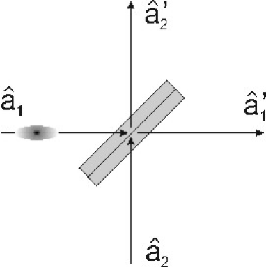
Figure 1: Beam splitter. The picture above shows a polarizing beam splitter. (Courtesy of Oliver Glöckl and Natasha Korolkova.) The picture below schematically illustrates the quantum theory of the beam splitter. Two incident light modes, represented by the Bose mode operators $\hat{a}_{1}$ and $\hat{a}_{2}$ interfere to produce two emerging modes with operators $\hat{a}_{1}^{\prime}$ and $\hat{a}_{2}^{\prime}$. Even if only one incident beam is split the vacuum noise of the second incident mode behind the mirror plays an important role in the quantum optics of the beam splitter.

The archetype of passive optical instruments is the beam splitter, usually an innocent-looking cube of glass in laboratory experiments, see Fig. 1. Light incident at the front of the cube is split into two beams, and so is light incident at the back. Both modes may interfere. In Sec. 2 we studied the theoretically simplest example of a beam splitter, a one-dimensional dielectric structure. Polarizers, where the two polarization modes of light are mixed, are also essentially beam splitters, and so are simple passive interferometers. The theory of this passive four-port device has been developed in Refs. [5, 4, 38, 41, 72, 76, 77, 78, 93, 102, 124, 138, 143, 145, 150, 155, 183, 199]. Here we follow mostly Refs. [41, 102]. More complicated optical multiports [156, 175, 177], where a multitude of beams interfere to produce the same number of outgoing modes, can be constructed from beam splitters and mirrors [156]. But already the simple beam splitter, combined with good photodetectors and single-photon sources, is quite capable of demonstrating some fundamental aspects of the wave-particle duality of light.

4.1 Matrix structure

The beam splitter is completely characterized by a unitary $2\times 2$ matrix $\underline{B}$ that describes how the device transforms the incident modes into the outgoing modes in the Heisenberg picture,

$$\left(\begin{array}[]{c}\hat{a}_{1}^{\prime}\\ \hat{a}_{2}^{\prime}\end{array}\right)=\underline{B}\left(\begin{array}[]{c}\hat{a}_{1}\\ \hat{a}_{2}\end{array}\right)\,,\quad\underline{B}=\left(\begin{array}[]{cc}B_{11}&B_{12}\\ B_{21}&B_{22}\end{array}\right)\,.$$ (4.1)

The beam-splitter matrix is unitary, in order to preserve the Bose commutation relations between the mode operators. Explicitly, the matrix elements must obey

$$|\,B_{11}\,|^{2}+|\,B_{12}\,|^{2}=1\,,\quad|\,B_{21}\,|^{2}+|\,B_{22}\,|^{2}=1\,,\quad B_{11}^{*}B_{21}+B_{12}^{*}B_{22}=0\,.$$ (4.2)

The general solution of these equations is

$$\underline{B}=e^{i\Lambda/2}\left(\begin{array}[]{cc}\cos(\Theta/2)\,e^{i(\Psi+\Phi)/2}&\sin(\Theta/2)\,e^{i(\Psi-\Phi)/2}\\ -\sin(\Theta/2)\,e^{i(\Phi-\Psi)/2}&\cos(\Theta/2)\,e^{-i(\Psi+\Phi)/2}\end{array}\right)$$ (4.3)

with the real parameters $\Phi$, $\Theta$, $\Psi$ and $\Lambda$. The one-dimensional dielectric structure with matrix (2.26) represents the special case where $\Phi=-\Psi$. We express the general beam-splitter matrix (4.3) as the product

$$\underline{B}=e^{i\Lambda/2}\left(\begin{array}[]{cc}e^{i\Psi/2}&0\\ 0&e^{-i\Psi/2}\end{array}\right)\left(\begin{array}[]{cc}\cos(\Theta/2)&\sin(\Theta/2)\\ -\sin(\Theta/2)&\cos(\Theta/2)\end{array}\right)\left(\begin{array}[]{cc}e^{i\Phi/2}&0\\ 0&e^{-i\Phi/2}\end{array}\right)\,.$$ (4.4)

The beam splitter acts in four steps. The incident modes gain a relative phase of $\Phi$, the modes are optically mixed with the mixing angle $\Theta/2$, and the outgoing modes attain the relative phase $\Psi$ and the overall phase $\Lambda/2$. We could incorporate the phases into the definitions of the incident and the outgoing modes. The rotation matrix would remain as the key feature of the beam splitter. The reflectivity $\varrho$ is characterized by $-\sin(\Theta/2)$ (the sign is unimportant though) while the transmissivity $\tau$ is given by $\cos(\Theta/2)$, which implies $\tau^{2}+\varrho^{2}=1$. The beam splitter has been assumed to be perfectly lossless — if a photon is not transmitted it must be reflected. We show in Sec. 5 how, in principle, absorption can be included and that the beam splitter itself serves as a convenient model of an absorber.

4.2 Quantum Stokes parameters

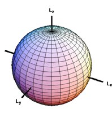
Figure 2: Poincaré sphere. The classical polarization of light is characterized by the Stokes parameters that lie on the Poincaré sphere. In quantum optics, the Jordan-Schwinger operators (4.17) play the role of the quantum Stokes parameters and their quantum statistics characterizes the polarization state. The parameter $\hat{L}_{t}$, the conserved total photon number, corresponds to the radius of the Poincaré sphere. The polarizer of Fig. 1 rotates the quantum Stokes parameters. In general, we can characterize the two incident modes of any beam splitter by their Jordan-Schwinger operators as well, and the beam splitter performs a rotation on the generalized Poincaré sphere.

The classical polarization of a light beam is usually described using the Stokes parameters [27]. Given the complex amplitudes $a_{1}$ and $a_{2}$ of the two polarization modes, the three Stokes parameters are proportional to the corresponding expectation values of the Pauli matrices

$$\sigma_{x}=\left(\begin{array}[]{cc}0&1\\ 1&0\end{array}\right)\,,\quad\sigma_{y}=\left(\begin{array}[]{cc}0&-i\\ i&0\end{array}\right)\,,\quad\sigma_{z}=\left(\begin{array}[]{cc}1&0\\ 0&-1\end{array}\right)\,.$$ (4.5)

The Stokes parameters lie on a sphere, the Poincaré sphere [27], also called the Bloch sphere in quantum mechanics [127], see Fig. 2. In quantum optics, we describe the polarization, the spinor part of the angular momentum of light, in terms of the quantum Stokes parameters [88]

$$\hat{L}_{t} = \frac{1}{2}\,(\hat{a}_{1}^{\dagger},\,\hat{a}_{2}^{\dagger})\,\,\mathds{1}\,\left(\begin{array}[]{c}\hat{a}_{1}\\ \hat{a}_{2}\end{array}\right)=\frac{1}{2}\,\left(\hat{a}_{1}^{\dagger}\hat{a}_{1}+\hat{a}_{2}^{\dagger}\hat{a}_{2}\right)\,,$$ (4.8)

$$\hat{L}_{x} = \frac{1}{2}\,(\hat{a}_{1}^{\dagger},\,\hat{a}_{2}^{\dagger})\,\sigma_{x}\left(\begin{array}[]{c}\hat{a}_{1}\\ \hat{a}_{2}\end{array}\right)=\frac{1}{2}\,\left(\hat{a}_{1}^{\dagger}\hat{a}_{2}+\hat{a}_{2}^{\dagger}\hat{a}_{1}\right)\,,$$ (4.11)

$$\hat{L}_{y} = \frac{1}{2}\,(\hat{a}_{1}^{\dagger},\,\hat{a}_{2}^{\dagger})\,\sigma_{y}\left(\begin{array}[]{c}\hat{a}_{1}\\ \hat{a}_{2}\end{array}\right)=\frac{i}{2}\,\left(\hat{a}_{2}^{\dagger}\hat{a}_{1}-\hat{a}_{1}^{\dagger}\hat{a}_{2}\right)\,,$$ (4.14)

$$\hat{L}_{z} = \frac{1}{2}\,(\hat{a}_{1}^{\dagger},\,\hat{a}_{2}^{\dagger})\,\sigma_{z}\left(\begin{array}[]{c}\hat{a}_{1}\\ \hat{a}_{2}\end{array}\right)=\frac{1}{2}\,\left(\hat{a}_{1}^{\dagger}\hat{a}_{1}-\hat{a}_{2}^{\dagger}\hat{a}_{2}\right)\,,$$ (4.17)

that obey the commutation relations of angular-momentum operators

$$[\hat{L}_{x},\,\hat{L}_{y}]=i\hat{L}_{z}\,,\quad[\hat{L}_{y},\,\hat{L}_{z}]=i\hat{L}_{x}\,,\quad[\hat{L}_{z},\,\hat{L}_{x}]=i\hat{L}_{y}\,.$$ (4.18)

Equation (4.17) is called the Jordan-Schwinger representation [83, 166] of the angular momentum in terms of two Bose operators. The representation serves as the starting point for the quantum theory of polarized or partially polarized light [88, 101]. The operator $\hat{L}_{t}$ commutes with all others and serves to represent the squared total angular momentum,

$$\hat{L}_{x}^{2}+\hat{L}_{y}^{2}+\hat{L}_{z}^{2}=\hat{L}_{t}(\hat{L}_{t}+1)\,.$$ (4.19)

The commutation relations (4.18) give rise to uncertainty relations between the quantum Stokes parameters. Polarization squeezing [69] occurs when the statistical fluctuations of one Stokes parameter are below the minimum-uncertainty limit. This quantum-noise reduction of the polarization of light has been applied to observe macroscopic spin-squeezing effects in atomic vapors [63, 84].

The Jordan-Schwinger representation (4.17) serves not only to characterize the polarization of quantum light, the representation provides also the theoretical tools to describe the effect of polarizers or of any beam splitter in general. We obtain from the commutation relations (4.18)

$$\exp(-i\Phi\hat{L}_{z})\left(\begin{array}[]{c}\hat{L}_{x}\\ \hat{L}_{y}\\ \hat{L}_{z}\end{array}\right)\exp(i\Phi\hat{L}_{z}) = \left(\begin{array}[]{ccc}\cos\Phi&\sin\Phi&0\\ -\sin\Phi&\cos\Phi&0\\ 0&0&1\end{array}\right)\left(\begin{array}[]{c}\hat{L}_{x}\\ \hat{L}_{y}\\ \hat{L}_{z}\end{array}\right)\,,$$ (4.29)

$$\exp(-i\Theta\hat{L}_{y})\left(\begin{array}[]{c}\hat{L}_{x}\\ \hat{L}_{y}\\ \hat{L}_{z}\end{array}\right)\exp(i\Theta\hat{L}_{y}) = \left(\begin{array}[]{ccc}\cos\Theta&0&\sin\Theta\\ 0&1&0\\ -\sin\Theta&0&\cos\Theta\end{array}\right)\left(\begin{array}[]{c}\hat{L}_{x}\\ \hat{L}_{y}\\ \hat{L}_{z}\end{array}\right)\,,$$ (4.39)

$$\exp(-i\Omega\hat{L}_{x})\left(\begin{array}[]{c}\hat{L}_{x}\\ \hat{L}_{y}\\ \hat{L}_{z}\end{array}\right)\exp(i\Omega\hat{L}_{x}) = \left(\begin{array}[]{ccc}1&0&0\\ 0&\cos\Omega&\sin\Omega\\ 0&-\sin\Omega&\cos\Omega\end{array}\right)\left(\begin{array}[]{c}\hat{L}_{x}\\ \hat{L}_{y}\\ \hat{L}_{z}\end{array}\right)\,,$$ (4.49)

as one easily verifies by differentiation with respect to the parameters. Therefore, the exponential Jordan-Schwinger operators describe rotations on the Poincare sphere, generated by polarizers. We note that the angles $\Phi$, $\Theta$, $\Psi$ in the complex matrix representation (4.3) are the Euler angles of an arbitrary rotation in three-dimensional space [96]. We obtain for the mode operators

$$\exp(-i\Phi\hat{L}_{z})\left(\begin{array}[]{c}\hat{a}_{1}\\ \hat{a}_{2}\end{array}\right)\exp(i\Phi\hat{L}_{z}) = \left(\begin{array}[]{cc}e^{i\Phi/2}&0\\ 0&e^{-i\Phi/2}\\ \end{array}\right)\left(\begin{array}[]{c}\hat{a}_{1}\\ \hat{a}_{2}\end{array}\right)\,,$$ (4.56)

$$\exp(-i\Theta\hat{L}_{y})\left(\begin{array}[]{c}\hat{a}_{1}\\ \hat{a}_{2}\end{array}\right)\exp(i\Theta\hat{L}_{y}) = \left(\begin{array}[]{cc}\cos(\Theta/2)&\sin(\Theta/2)\\ -\sin(\Theta/2)&\cos(\Theta/2)\\ \end{array}\right)\left(\begin{array}[]{c}\hat{a}_{1}\\ \hat{a}_{2}\end{array}\right)\,,$$ (4.63)

$$\exp(-i\Omega\hat{L}_{x})\left(\begin{array}[]{c}\hat{a}_{1}\\ \hat{a}_{2}\end{array}\right)\exp(i\Omega\hat{L}_{x}) = \left(\begin{array}[]{cc}\cos(\Omega/2)&i\sin(\Omega/2)\\ i\sin(\Omega/2)&\cos(\Omega/2)\\ \end{array}\right)\left(\begin{array}[]{c}\hat{a}_{1}\\ \hat{a}_{2}\end{array}\right)\,,$$ (4.70)

in agreement with our previous result (3.29) for the effective Hamiltonian of the real beam splitter (3.26). Consequently, the beam splitter performs rotations in the three-dimensional space spanned by the quantum Stokes parameters (4.17). Such rotations are independent on the overall phase $\Lambda/2$ in the factorization (4.4). For rotations on the quantum Poincaré sphere we can thus restrict the beam-splitter transformations to SU(2) matrices [48] with

$$\mathrm{det}\underline{B}=1\,.$$ (4.71)

Finally, we arrive at the general evolution operator for the beam splitter with matrix (4.4)

$$\hat{B}=\exp(-i\Phi\hat{L}_{z})\,\exp(-i\Theta\hat{L}_{y})\,\exp(-i\Psi\hat{L}_{z})\,\exp(-i\Lambda\hat{L}_{t})\,.$$ (4.72)

4.3 Wave-particle dualism

Now we possess the theoretical tools to predict what happens when two beams of quantum light interfere at a beam splitter. In classical optics, the light beams are characterized by their spatial shapes, by their normalized spatial mode functions $u_{1}$ and $u_{2}$, and by their amplitudes $a_{1}$ and $a_{2}$. The outgoing modes have the amplitudes

$$\left(\begin{array}[]{c}a_{1}^{\prime}\\ a_{2}^{\prime}\end{array}\right)=\underline{B}\left(\begin{array}[]{c}a_{1}\\ a_{2}\end{array}\right)\,.$$ (4.73)

The amplitudes of the incident light modes may statistically fluctuate if the beams are not perfectly coherent [27, 127]. In this case the outgoing modes fluctuate accordingly, because the individual amplitudes are transferred according to the relation (4.73). In quantum optics, the observables such as the amplitudes $\hat{a}_{1}$ and $\hat{a}_{2}$ or the photon numbers $\hat{a}_{1}^{\dagger}\hat{a}_{1}$ and $\hat{a}_{2}^{\dagger}\hat{a}_{2}$ may statistically fluctuate in repeated experiments, even if the light has always been prepared in identical pure states [110]. Such quantum fluctuations tend to be quite subtle and hard to discriminate from classical noise in experiments. The quantum-noise properties distinguish the various quantum states of light [110]. The coherent states [110] resemble classical light beams with well-defined amplitudes, coherent light. A coherent state of light is characterized by the Wigner function [110]

$$W(q,p)=\frac{1}{\pi}\,\exp\left(-(q-q_{0})^{2}-(p-p_{0})^{2}\right)=\frac{1}{\pi}\,\exp\left(-2|\,\alpha-a_{0}|^{2}\right)\,,$$ (4.74)

where $a_{0}=(q_{0}+ip_{0})/\sqrt{2}$ denotes the classical amplitude of the light beam and $\alpha$ abbreviates $(q+ip)/\sqrt{2}$. The Wigner function (4.74) describes the quantum-statistical fluctuations of the amplitude components $q$ and $p$, the quadratures [110]. The vacuum state belongs to the class of coherent states as well [110] — the vacuum is the coherent state with zero average amplitude. Yet the field amplitudes of the vacuum state still fluctuate [110]. We see from the Wigner function (4.74) that the amplitudes of coherent states fluctuate precisely like the quantum vacuum around their average values $a_{0}$. The coherent states are the most classical-like states of light, corresponding to waves as perfect as quantum mechanics allows. Note that the number of photons fluctuates in a coherent state, because precision in amplitude and precision in particle number are mutually exclusive. The photons in a coherent state of amplitude $a_{0}$ are as randomly distributed as raisins in a cake with $|\,a_{0}|^{2}$ apiece [110]. Technically [110], the photons follow a Poisson distribution around the average $|\,a_{0}|^{2}$.

Suppose that the two light beams incident on the beam splitter are in coherent states with the amplitudes $a_{1}$ and $a_{2}$, corresponding to the two-mode Wigner function

$$W(\alpha_{1},\alpha_{2})=\frac{1}{\pi^{2}}\,\exp\left(-2|\,\alpha_{1}-a_{1}|^{2}-2|\,\alpha_{2}-a_{2}|^{2}\right)\,.$$ (4.75)

To predict the quantum state of the outgoing modes, we apply the transformation rule (3.40) to the Wigner function (4.75) and utilize the unitarity (2.27) of the beam-splitter matrix. We obtain

$$W^{\prime}(\alpha_{1},\alpha_{2})=\frac{1}{\pi^{2}}\,\exp\left(-2|\,\alpha_{1}-a_{1}^{\prime}|^{2}-2|\,\alpha_{2}-a_{2}^{\prime}|^{2}\right)\,.$$ (4.76)

The outgoing modes are in coherent states with the amplitudes classically transformed (4.73). The modes are completely uncorrelated, because the Wigner function factorizes. The coherent states thus interfere just like classical waves, even down to the finest details of their quantum-statistical properties. This result uniquely distinguishes coherent states [4] and it can be extended to any passive optical network [156, 175, 177]. Historically, the interference property of coherent states has been deduced from a microscopic model of the beam splitter [38] and has served as the starting point for the quantum theory of such optical instruments [143].

Now, suppose that one incident beam carries precisely $n$ photons and that no light impinges on the back of the semi-transparent mirror. The light beam with exactly $n$ photons is in the Fock state [110]

$$|\,n\,\rangle=\frac{1}{\sqrt{n!}}\,\hat{a}^{\dagger n}|\,0\,\rangle\,,$$ (4.77)

and the other incident mode is in the vacuum state $|\,0\,\rangle$. Fock states are the eigenstates of the photon-number operator $\hat{a}^{\dagger}\hat{a}$ and hence they correspond to light with a perfectly well-defined number of photons [110]. We calculate the quantum state of the outgoing modes

$$\hat{B}^{\dagger}|\,n\,\rangle_{1}\,|\,0\,\rangle_{2}=\frac{1}{\sqrt{n!}}\,\hat{B}^{\dagger}\hat{a}^{\dagger n}|\,0\,\rangle_{1}\,|\,0\,\rangle_{2}=\frac{1}{\sqrt{n!}}\,\hat{B}^{\dagger}\hat{a}^{\dagger n}\hat{B}\,|\,0\,\rangle_{1}\,|\,0\,\rangle_{2}\,.$$ (4.78)

Here we have used the fact that the beam splitter transforms the incident vacuum into the outgoing vacuum, ex nihilo nihil, as we easily see from the Wigner function (4.76) with zero initial amplitudes $a_{1}$ and $a_{2}$. Since

$$\hat{B}^{\dagger}\left(\begin{array}[]{c}\hat{a}_{1}\\ \hat{a}_{2}\end{array}\right)\hat{B}=\underline{B}^{-1}\left(\begin{array}[]{c}\hat{a}_{1}\\ \hat{a}_{2}\end{array}\right)=\left(\begin{array}[]{cc}B_{11}^{*}&B_{21}^{*}\\ B_{12}^{*}&B_{22}^{*}\end{array}\right)\left(\begin{array}[]{c}\hat{a}_{1}\\ \hat{a}_{2}\end{array}\right)\,,$$ (4.79)

we obtain according to the Binomial theorem and the definition (4.77) of the Fock states

$$\hat{B}^{\dagger}|\,n\,\rangle_{1}\,|\,0\,\rangle_{2} = \frac{1}{\sqrt{n!}}\,\left(B_{11}\,\hat{a}_{1}^{\dagger}+B_{21}\,\hat{a}_{2}^{\dagger}\right)^{n}\,|\,0\,\rangle_{1}\,|\,0\,\rangle_{2}$$ (4.82)

$$= \sum_{k=0}^{n}\sqrt{\left(\begin{array}[]{c}n\\ k\end{array}\right)}B_{11}^{k}\,B_{21}^{n-k}\,|\,k\,\rangle_{1}\,|\,n-k\,\rangle_{2}\,,$$

$$\left(\begin{array}[]{c}n\\ k\end{array}\right)=\frac{n!}{(n-k)!k!}\,.$$ (4.83)

The beam splitter does not split the incident photons, of course, but rather the semi-transparent mirror statistically distributes the photons into the reflected and the transmitted beam. Suppose we count the photons in each emerging mode [32]. Each individual run of the experiment [32] is unpredictable, but averaged over a large statistical ensemble we get the joint photon-number distribution

$$p(n_{1},n_{2})=\left(\begin{array}[]{c}n\\ k\end{array}\right)\tau^{2k}\,(1-\tau^{2})^{n-k}\,\delta_{n_{1},\,k}\,\delta_{n_{2},\,n-k}\,,$$ (4.84)

where $\tau$ denotes the transmissivity $|B_{11}|$. The Binomial distribution (4.84) describes a random decision process where $n$ distinguishable objects are distributed to two channels, to the first channel with probability $\tau^{2}$ per object and to the second one with probability $1-\tau^{2}$, accordingly, because the beam splitter is assumed to be perfectly lossless. Each photon is statistically independent, and so the probability for $k$ individual photons to arrive in the first channel and $n-k$ photons in the second one is the product $\tau^{2k}\,(1-\tau^{2})^{n-k}$. We multiply this value by the Binomial coefficient, which describes the number of possibilities to distribute any $k$ of the $n$ photons to the first channel and the rest to the second one, because we cannot discriminate between individual photons in photon-counting experiments. Nevertheless, photons behave in beam-splitting experiments as if they were in-principle distinguishable, in contrast to the common statement that photons are fundamentally indistinguishable particles, which illustrates some of the conceptional subtleties of the photon.

There is another twist in the physics of photons and the beam splitter. Suppose you let two beams of light with equal intensities interfere at a perfect 50:50 beam splitter characterized by the real matrix

$$\underline{B}=\left(\begin{array}[]{cc}{1}/{\sqrt{2}}&{1}/{\sqrt{2}}\\ -{1}/{\sqrt{2}}&{1}/{\sqrt{2}}\end{array}\right)\,.$$ (4.85)

Consider two coherent states with equal complex amplitudes $a_{0}=a_{1}=a_{2}$. We obtain from the transformation rule (4.73) that the first outgoing mode is in the coherent state with complex amplitude $\sqrt{2}\,a_{0}$, whereas the second mode is in the vacuum state. The two incident light beams interfere constructively in the first outgoing mode and destructively in the second one. If the two incident coherent states have equal amplitudes but opposite phases, $a_{1}=a_{0}$, $a_{2}=-a_{0}$, they interfere the other way round. Now, suppose you let one single photon interfere with another single photon. We calculate the quantum state of the outgoing modes,

$$\hat{B}^{\dagger}|\,1\,\rangle_{1}\,|\,1\,\rangle_{2} = \frac{1}{2}\,\left(\hat{a}_{1}^{\dagger}-\hat{a}_{2}^{\dagger}\right)\,\left(\hat{a}_{1}^{\dagger}+\hat{a}_{2}^{\dagger}\right)\,|\,0\,\rangle_{1}\,|\,0\,\rangle_{2}$$ (4.86)

$$= \frac{1}{\sqrt{2}}\Big{(}|\,2\,\rangle_{1}\,|\,0\,\rangle_{2}-|\,0\,\rangle_{1}\,|\,2\,\rangle_{2}\Big{)}\,.$$

The photons interfere constructively or destructively. Complete destructive interference implies that the affected outgoing mode is in the vacuum state, whereas the other mode must carry exactly two photons, because the total number of photons is conserved. Destructive or constructive interference depends on the relative phase of the incident photons. Fock states with precisely defined photon number are the most extreme particle-like states of light, and hence they do not carry any wave-like phase information. Faced with this dilemma, the beam splitter distributes the two photons in either way with $1/\sqrt{2}$ probability amplitude, i.e. with $50\%$ probability after detection, a truly Solomonic solution. Experimentally [71], the coincident counts of photons reach a well-pronounced minimum when the spatial-temporal modes of the incident photons overlap at the beam splitter. The choice which one of the outgoing mode carries the two photons becomes only apparent when the light is detected. The same is true for the beam splitting of $n$ photons discussed previously. The beam splitter itself is a deterministic device. The probabilistic outcome of the photocounting remains undecided until the measurement is made. The quantum state (4.86) of the outgoing modes is strongly correlated, and so is the state (4.82) of the split Fock state, in contrast to the interference (4.76) of coherent states. Moreover, the decisive measurement devices may be located a long distance apart from each other. Both photon-interference and photon-splitting experiments are suitable [172, 64] to test the non-locality of quantum mechanics [20, 51].

5 Absorber and amplifier

The optical instruments studied so far are completely reversible devices. For example, when a Fock state, carrying a precise number of photons, is split at a beam splitter we could, in principle, send the outgoing beams back to restore the initial Fock state. Mathematically argued, the instruments (3.1) are reversible, because the quasi-unitary $\underline{S}$ matrix has the inverse $\underline{G}\,\underline{S}^{\dagger}\underline{G}$, according to Eq. (3.4). So far, we have excluded irreversible processes such as the absorption or the amplification of light. However, all quantum processes are fundamentally reversible, as long as no measurements are made or could be made in principle (whatever measurement processes are), and as long as we keep track of the quantum systems involved.

Consider for example an absorber, a piece of grey material. Some of the incident light is destined for absorption and some part is transmitted, with reduced intensity though. The absorbed component is transferred to the material and ebbs away in many small material excitations as heat. Normally we are simply not able to keep track of the material details and so the absorbed quanta are lost. (Exceptions are very simple atomic systems, two-level systems for example, where absorption is reversible [79, 142, 169].) The first part of the absorption process resembles beam splitting. We could model the second, the irreversible part by discarding the quantum information carried in one of the outgoing beams, i.e. by averaging over the unobserved component of the total quantum system. Modeling absorption and detection losses by fictitious beam splitters has been a successful idea in quantum optics [53, 80, 86, 103, 145, 194]. This theoretical trick is known elsewhere as the thermo-field technique [180]. In fact, many absorbers are first of all scatterers, but it is quite remarkable that we can sum up the multitude of scattered light modes in just one outgoing mode of a fictitious beam splitter. Moreover, an absorber may emit thermal radiation according to its temperature, and so we should include emission as well as absorption in our model. When the stimulated emission dominates the device acts as an amplifier. To understand how to model such irreversible processes requires some theory [33, 42, 56, 57, 120].

5.1 Lindblad’s theorem

Lindblad [120] determined the most general structure of the dynamic equation for the density operator $\hat{\rho}$, assuming only that the evolving $\hat{\rho}$ represents indeed an ensemble of pure quantum states $|\,\psi_{a}\rangle$ occuring with probabilities $p_{a}$. A reversible quantum process would only change the pure states $|\,\psi_{a}\rangle$ while an irreversible process may affect both the $|\,\psi_{a}\rangle$ and their probabilities $p_{a}$. Lindblad’s master equation, the quantum version of the Boltzmann equation, reads [33, 42, 56, 57, 120]

$$\partial_{t}\hat{\rho}=\frac{i}{\hbar}\,[\hat{\rho},\hat{H}_{0}]-\sum_{l}\gamma_{l}\left(\hat{L}_{l}^{\dagger}\hat{L}_{l}\hat{\rho}-2\hat{L}_{l}\hat{\rho}\hat{L}_{l}^{\dagger}+\hat{\rho}\hat{L}_{l}^{\dagger}\hat{L}_{l}\right)\,.$$ (5.1)

Here $\hat{H}_{0}$ denotes the Hamiltonian of the reversible part of the dynamics, while the $\gamma_{l}$ quantify the rates of the irreversible processes described by the Lindblad operators $\hat{L}_{l}$. The parameter $t$ may describe a fictitious time that, for example, corresponds to the penetration depth of an absorbing material or to the length of a laser amplifier. We define the effective Hamiltonian

$$\hat{H}_{\rm eff}=\hat{H}_{0}-i\hbar\sum_{l}\gamma_{l}\hat{L}_{l}^{\dagger}\hat{L}_{l}\,,$$ (5.2)

a non-Hermitian operator, and write the master equation (5.1) as

$$\partial_{t}\hat{\rho}=\frac{i}{\hbar}\left(\hat{\rho}\hat{H}_{\rm eff}^{\dagger}-\hat{H}_{\rm eff}\hat{\rho}\right)+2\sum_{l}\gamma_{l}\hat{L}_{l}\hat{\rho}\hat{L}_{l}^{\dagger}\,.$$ (5.3)

The effective Hamiltonian alone would reduce the total quantum probability $\mathrm{tr}\hat{\rho}$. The component $i(\hat{\rho}\hat{H}_{\rm eff}^{\dagger}-\hat{H}_{\rm eff}\hat{\rho})/\hbar$ of the master equation (5.3) describes the coherent part of the irreversible process, for example damping or amplification, while the terms $2\gamma_{l}\hat{L}_{l}\hat{\rho}\hat{L}_{l}^{\dagger}$ characterize the effect of quantum jumps [33, 42], fluctuations that restore the nature of the density operator. In this respect, Lindblad’s theorem [120] formulates the quantum version of the fluctuation-dissipation theorem [99].

The Lindblad operators $\hat{L}_{l}$ describe the specific physical effects of the irreversible processes involved in the dynamics (5.1), the quantum transitions caused. In short, the $\hat{L}_{l}$ are the transition operators. For specific irreversible processes we can frequently use our intuition to infer the relevant transition operators. We may guess that the absorption of light corresponds to the effect of the annihilation operator $\hat{a}$, while the light emission is represented by the creation operator $\hat{a}^{\dagger}$. An absorber or amplifier is thus modeled by the Lindblad operators

$$\hat{L}_{1}=\hat{a}\,,\quad\hat{L}_{2}=\hat{a}^{\dagger}\,.$$ (5.4)

For simplicity, we ignore the Hamiltonian $\hat{H}_{0}$ of the single light mode that would only generate a time-dependent phase shift of light. We translate the master equation (5.1) with the Lindblad operators (5.4) into the evolution equation of the Wigner function, a Fokker-Planck equation [42, 56, 57, 159]. For this, we express the master equation in terms of the quadratures $\hat{q}$ and $\hat{p}$ with $\hat{a}=(\hat{q}+i\hat{p})/\sqrt{2}$ and calculate the Wigner transforms (3.35) of the operators involved. We use the correspondence rules [56]

$$\hat{q}\hat{F}\longleftrightarrow\left(q+\frac{i}{2}\,\partial_{p}\right)W_{F} \quad\hat{F}\hat{q}\longleftrightarrow\left(q-\frac{i}{2}\,\partial_{p}\right)W_{F}\,,$$ ,

$$\hat{p}\hat{F}\longleftrightarrow\left(p-\frac{i}{2}\,\partial_{q}\right)W_{F} \quad\hat{F}\hat{p}\longleftrightarrow\left(p+\frac{i}{2}\,\partial_{q}\right)W_{F}\,,$$ , (5.5)

between the operators and their Wigner transforms, and arrive at the Fokker-Planck equation

$$\partial_{t}W=(\gamma_{1}-\gamma_{2})\big{(}\partial_{q}(qW)+\partial_{p}(pW)\big{)}+\frac{\gamma_{1}+\gamma_{2}}{2}\big{(}\partial_{q}^{2}W+\partial_{p}^{2}W\big{)}\,.$$ (5.6)

The first term, with prefactor $\gamma_{1}-\gamma_{2}$, describes the drift of the quasiprobabilities, to zero if the absorption dominates and to infinity if the emission is stronger. The second term, with rate $(\gamma_{1}+\gamma_{2})/2$, describes the diffusion of the quasiprobabilities due to quantum noise.

5.2 Absorber

Suppose that the absorption rate $\gamma_{1}$ outweighs the emission rate $\gamma_{2}$. In this case, the Fokker-Planck equation (5.6) describes the net effect of an absorber. We find the stationary solution, normalized to unity,

$$W_{\mathrm{th}}(q,p)=\frac{1}{\pi(2N+1)}\,\exp\left(-\frac{q^{2}+p^{2}}{2N+1}\right)\,,\quad 2N+1=\left|\frac{\gamma_{1}+\gamma_{2}}{\gamma_{1}-\gamma_{2}}\right|\,.$$ (5.7)

The Wigner function $W_{\mathrm{th}}$ corresponds to the thermal state [110]

$$\hat{\rho}=\frac{N}{N+1}\,\exp\left(-\frac{\hbar\omega\hat{a}^{\dagger}\hat{a}}{k_{\mathrm{B}}T}\right)$$ (5.8)

with average photon number $N$ and temperature $T$, according to Planck’s formula

$$N=\left[\exp\left(\frac{\hbar\omega}{k_{\mathrm{B}}T}\right)-1\right]^{-1}\,.$$ (5.9)

The stationary solution indicates that the absorber consists of a thermal reservoir with temperature $T$, a reservoir that absorbs light, but that also emits thermal radiation. Now, consider the general solution of the Fokker-Planck equation (5.6). One verifies easily that the solution is [102]

$$W(\alpha,t)=\int_{-\infty}^{+\infty}\int_{-\infty}^{+\infty}W(\alpha_{1}^{\prime},t_{0})\,W_{\mathrm{th}}(\alpha_{2}^{\prime})\,\mathrm{d}q_{0}\,\mathrm{d}p_{0}\,,$$ (5.10)

where the $\alpha$’s abbreviate the $(q+ip)/\sqrt{2}$ amplitudes, with

$$\left(\begin{array}[]{c}\alpha_{1}^{\prime}\\ \alpha_{2}^{\prime}\end{array}\right)=\left(\begin{array}[]{cc}\sqrt{\eta}&-\sqrt{1-\eta}\\ \sqrt{1-\eta}&\sqrt{\eta}\end{array}\right)\left(\begin{array}[]{c}\alpha\\ \alpha_{0}\end{array}\right)$$ (5.11)

and

$$\eta=\exp\left[-2(\gamma_{1}-\gamma_{2})(t-t_{0})\right]\,,\quad t\geq t_{0}\,.$$ (5.12)

Any initial Wigner function $W(\alpha,t_{0})$ is exponentially attenuated and eventually approaches the thermal state $W_{\mathrm{th}}$ in the limit $t\rightarrow+\infty$. The result (5.10) with the relation (5.11) proves that partial absorption corresponds to a simple beam splitter model. The incident light appears to be split into the transmitted and the absorbed component. The $\eta$ parameter (5.12) describes the transmission probability of a single photon and $1-\eta$ is the probability of absorption. The second mode of the fictitious beam splitter plays a double role. The mode represents the reservoir into which the absorbed light disappears and over which we average in the solution (5.10). Additionally, the initial state of the mode describes the fluctuations of the thermal reservoir that contaminate the transmitted light. In the Heisenberg picture we represent the mode operator of the partially absorbed light as

$$\hat{a}(t)=\hat{a}(t_{0})\sqrt{\eta}+\hat{a}_{0}\sqrt{1-\eta}\,.$$ (5.13)

The fluctuation mode is essential in order to preserve the Bose commutation relation of $\hat{a}(t)$, even at zero temperature. Usually, for light in the optical range of the spectrum, room temperature and zero temperature makes little difference. In this case, the vacuum fluctuations of the reservoir affect the partially absorbed light. If the light has initially been in a coherent state with amplitude $a_{0}$ the transmitted light remains in a coherent state with the reduced amplitude $\sqrt{\eta}\,a_{0}$, despite the vacuum fluctuations, because, as we know, the beam splitter transforms coherent states (the initial state and the vacuum mode) into disentangled coherent states. On the other hand, other quantum states approach coherent states during the absorption process. The absorber purifies light with excess amplitude noise, but the absorber also destroys fragile non-classical states with unusual quantum properties, such as Schrödinger-cat states [37, 102].

5.3 Amplifier

Suppose that the emission rate $\gamma_{2}$ outweighs the absorption rate $\gamma_{1}$ in the irreversible process (5.1) with the Lindblad operators (5.4). In this case the Fokker-Planck equation (5.6) has the general solution (5.10) with [104]

$$\left(\begin{array}[]{c}\alpha_{1}^{\prime}\\ \alpha_{2}^{\prime*}\end{array}\right)=\left(\begin{array}[]{cc}\sqrt{\eta}&-\sqrt{\eta-1}\\ -\sqrt{\eta-1}&\sqrt{\eta}\end{array}\right)\left(\begin{array}[]{c}\alpha\\ \alpha_{0}^{*}\end{array}\right)$$ (5.14)

and with the $\eta$ parameter (5.12) larger than unity. The amplitude $\alpha$ of the initial Wigner function grows with $\sqrt{\eta}$ and exponentially in $t$, which indicates that the process describes a linear amplifier with gain $\eta=\exp[2(\gamma_{2}-\gamma_{1})(t-t_{0})]$. The amplification is accompanied by amplification noise, usually spontaneous-emission noise in laser amplifiers, summed up in the thermal Wigner function (5.7) that becomes interwoven with the initial quantum state. The noise temperature (5.9) characterizes the quality of the amplifier. Amplification noise is stronger than absorption noise in the sense that amplified coherent states do not remain coherent states, even at zero noise temperature. Therefore, amplification does not simply reverse attenuation. The growth of the signal mode combined with the inevitable amplification noise appears in the Heisenberg picture as

$$\hat{a}(t)=\hat{a}(t_{0})\sqrt{\eta}+\hat{a}_{0}^{\dagger}\sqrt{\eta-1}\,.$$ (5.15)

As in the case of the absorber, the fluctuation mode preserves the Bose commutation relation of the amplified light, but the amplification noise always creates additional quanta, indicated by the creation operator, in contrast to the absorption noise.

Suppose that the amplifier attempts to balance the effect of attenuation, i.e. $\gamma_{1}=\gamma_{2}=\gamma$ in the process (5.1) with the Lindblad operators (5.4). Imagine, for example, that Eve, the eavesdropper, tries to tap quantum information by beam splitting while covering up her tracks by amplification. In the case when the emission rate is equal to the absorption rate the Fokker-Planck equation (5.6) reduces to the pure diffusion of the Wigner function, without drift, as designed. We calculate the quantum-statistical purity [56, 110] of the signal state using the overlap formula (3.36)

$$\mathrm{tr}\{\hat{\rho}^{2}\}=2\pi\int_{-\infty}^{+\infty}\int_{-\infty}^{+\infty}W^{2}\,\mathrm{d}q\,\mathrm{d}p\,,$$ (5.16)

and obtain from the Fokker-Planck equation (5.6) by partial integration

$$\partial_{t}\mathrm{tr}\{\hat{\rho}^{2}\}=-4\pi\gamma\int_{-\infty}^{+\infty}\int_{-\infty}^{+\infty}\Big{(}(\partial_{q}W)^{2}+(\partial_{p}W)^{2}\Big{)}\mathrm{d}q\,\mathrm{d}p<0\,.$$ (5.17)

The purity $\mathrm{tr}\{\hat{\rho}^{2}\}$ monotonously decreases until the Wigner function has been completely leveled by diffusion, containing no information anymore. Eavesdropping spoils the purity of the quantum state.

To summarize, both the attenuation and the amplification of light correspond to simple analog models that exactly describe the quantum effects of such irreversible processes. An absorber is represented by a beam splitter and an amplifier by a parametric amplifier. The second mode of the beam splitter represents the absorption reservoir, while the additional fluctuation mode of the amplifier describes the amplification noise. We have proven [102, 104] the equivalence between these simple models and the master equation (5.1) for the Lindblad operators (5.4), i.e. for thermal reservoirs. We can easily extend [102, 104] our analog models to phase-sensitive Gaussian reservoirs [56] with the squeezed Lindblad operators

$$\hat{L}_{1}=\mu\hat{a}+\nu\hat{a}^{\dagger}\,,\quad\hat{L}_{2}=\hat{L}_{1}^{\dagger}\,,\quad|\mu|^{2}-|\nu|^{2}=1\,,$$ (5.18)

characterized by the complex constants $\mu$ and $\nu$, see Refs. [102, 104] and Refs. cited therein. The transformation (5.18) squeezes the thermal Wigner function (5.7) of the quantum noise in one phase-space direction and stretches it in the orthogonal direction, indicating that the reservoir is indeed phase sensitive, possibly with reduced fluctuations in one of the quadratures. The fluctuation mode is in a state with Gaussian Wigner function and Gaussian density operator [56]. Whether our simple models can be extended beyond Gaussian reservoirs remains unknown.

6 Parametric amplifier

The prime example of an active linear device is the optical parametric amplifier [168]. Phase-conjugating mirrors [168] and four-wave mixers [168] belong to the same category. The quantum optics of parametric amplifiers is studied in Refs. [43, 73, 80, 119, 132, 133, 144, 179, 198], the quantum properties of phase-conjugating mirrors are considered in Refs. [2, 3, 22, 54, 139] and the quantum effects of four-wave mixers are studied in Refs. [89, 157, 195, 197]. Active devices require external energy sources, often provided by other light beams. These pump beams interact with the modes to be amplified in non-linear media [26, 168], mostly certain crystals in the case of parametric amplifiers. The modes are linearly amplified, as long as they do not feed back to the pump processes. Here we focus entirely on the regime of linear amplification. The quantum physics of pump depletion has been analyzed in Refs. [10, 11].

The simplest example for parametric amplification in physics is the playground swing. Rocking the legs changes the moment of intertia. Rocking with twice the fundamental frequency of the swing amplifies the oscillation, starting from tiny initial movements, a phenomenon called parametric resonance [96]. The simplest optical example of a parametric amplifier is the downconverter [127]. Pump light with frequency $\omega_{p}$ drives two other beams of light, called the signal and the idler, with frequencies $\omega_{s}+\omega_{i}=\omega_{p}$. Assisted by the non-linear medium, some pump photons with energy $\hbar\omega_{p}$ decay into photon pairs with energies $\hbar\omega_{s}$ and $\hbar\omega_{i}$. The Hamiltonian (3.33) describes such a process, the creation of photon pairs. The Hamiltonian also accounts for the reverse process where photon pairs become annihilated with their energies transferred back to the pump. The relative phase between the signal, idler and pump beams decides the direction of the process. Furthermore, momentum conservation requires that the wave vectors ${\bf k}_{p}$ of the pump light should equal the sum of the wave vectors of signal and idler, ${\bf k}_{s}$ and ${\bf k}_{i}$, a condition called phase matching [168]. Parametric amplifiers with high quantum-noise quality and efficiency tend to take pure crystals, good resonators and a number of ingenious experimental tricks.

6.1 Matrix structure and squeezing

The Hamiltonian (3.33) of the downconverter generates the linear mode transformation (3.1) with the $\underline{S}$ matrix (3.30). The mode operator of the signal, say $\hat{a}_{1}$, is mixed with the Hermitian conjugate of the idler, $\hat{a}_{2}^{\dagger}$. Simultaneously, the idler operator $\hat{a}_{2}$ is mixed with the conjugate of the signal, $\hat{a}_{1}^{\dagger}$. We would expect the same for phase-conjugating mirrors [168]. Let us assume the mode transformation

$$\left(\begin{array}[]{c}\hat{a}_{1}^{\prime}\\ \hat{a}_{2}^{\prime\dagger}\end{array}\right)=\underline{B}\left(\begin{array}[]{c}\hat{a}_{1}\\ \hat{a}_{2}^{\dagger}\end{array}\right)\,,\quad\underline{B}=\left(\begin{array}[]{cc}B_{11}&B_{12}\\ B_{21}&B_{22}\end{array}\right)\,,$$ (6.1)

corresponding to the $\underline{S}$ matrix

$$\underline{S}=\left(\begin{array}[]{cccc}B_{11}&0&0&B_{12}\\ 0&B_{22}^{*}&B_{21}^{*}&0\\ 0&B_{12}^{*}&B_{11}^{*}&0\\ B_{21}&0&0&B_{22}\end{array}\right)\,.$$ (6.2)

The mode transformation (6.1) describes pure amplification, without scattering. We require that the mode operators of both the incident and the amplified light are proper Bose operators, which results in the quasi-unitarity relation (3.4) of the $\underline{S}$ matrix. Explicitly, we obtain

$$|\,B_{11}\,|^{2}-|\,B_{12}\,|^{2}=1\,,\quad|\,B_{21}\,|^{2}-|\,B_{22}\,|^{2}=1\,,\quad B_{11}^{*}B_{21}-B_{12}^{*}B_{22}=0\,.$$ (6.3)

The general solution of these equations is

$$\underline{B}=e^{i\Lambda/2}\left(\begin{array}[]{cc}\cosh(\Theta/2)\,e^{i(\Psi+\Phi)/2}&\sinh(\Theta/2)\,e^{i(\Psi-\Phi)/2}\\ \sinh(\Theta/2)\,e^{i(\Phi-\Psi)/2}&\cosh(\Theta/2)\,e^{-i(\Psi+\Phi)/2}\end{array}\right)$$ (6.4)

with the real parameters $\Phi$, $\Theta$, $\Psi$ and $\Lambda$. We express $\underline{B}$ as the product

$$\underline{B}=e^{i\Lambda/2}\left(\begin{array}[]{cc}e^{i\Psi/2}&0\\ 0&e^{-i\Psi/2}\end{array}\right)\left(\begin{array}[]{cc}\cosh(\Theta/2)&\sinh(\Theta/2)\\ \sinh(\Theta/2)&\cosh(\Theta/2)\end{array}\right)\left(\begin{array}[]{cc}e^{i\Phi/2}&0\\ 0&e^{-i\Phi/2}\end{array}\right)\,.$$ (6.5)

Like in the case of the beam splitter, the net result of the parametric amplifier or of the phase-conjugating mirror amounts to four steps. First, the incident beams gain a phase $\Phi/2$, yet in contrast to the beam splitter, this is not a relative phase, but an absolute phase shift, because the transformation (6.1) acts on $\hat{a}_{1}$ and $\hat{a}_{2}^{\dagger}$, not on $\hat{a}_{1}$ and $\hat{a}_{2}$. After the phase shift the modes are amplified by the factor $\cosh(\Theta/2)$ and mixed, with the overlap $\sinh(\Theta/2)$, and finally the outgoing modes gain the absolute phase $\Psi/2$ and the relative phase $\Lambda$. We could include the phases into the definitions of the incident and the amplified modes. The hyperbolic mixing (3.30) would remain as the key feature of the device. We can express the $\underline{S}$ matrix (3.30) with $\zeta=\Theta/2$ as

$$\underline{S}=\underline{R}^{-1}\left(\begin{array}[]{cccc}\cosh(\Theta/2)&0&\sinh(\Theta/2)&0\\ 0&\cosh(\Theta/2)&0&-\sinh(\Theta/2)\\ \sinh(\Theta/2)&0&\cosh(\Theta/2)&0\\ 0&-\sinh(\Theta/2)&0&\cosh(\Theta/2)\end{array}\right)\underline{R}$$ (6.6)

in terms of the matrix of the 50:50 beam splitter (4.85)

$$\underline{R}=\left(\begin{array}[]{cccc}{1}/{\sqrt{2}}&{1}/{\sqrt{2}}&0&0\\ -{1}/{\sqrt{2}}&{1}/{\sqrt{2}}&0&0\\ 0&0&{1}/{\sqrt{2}}&{1}/{\sqrt{2}}\\ 0&0&-{1}/{\sqrt{2}}&{1}/{\sqrt{2}}\end{array}\right)\,.$$ (6.7)

In the case when the signal and the idler modes are the linear polarization modes of a single light wave the matrix $\underline{R}$ describes the rotation of the polarization axis by $\pi/4$. The parametric amplifier thus processes the rotated modes separately

$$\hat{a}_{r1}^{\prime}=\hat{a}_{r1}\cosh(\Theta/2)+\hat{a}_{r1}^{\dagger}\sinh(\Theta/2)\,,\quad\hat{a}_{r2}^{\prime}=\hat{a}_{r2}\cosh(\Theta/2)-\hat{a}_{r2}^{\dagger}\sinh(\Theta/2)\,.$$ (6.8)

We obtain for the quadratures (2.10)

$$\hat{q}_{r1}^{\prime}=\hat{q}_{r1}\,e^{+\Theta/2}\,,\quad\hat{p}_{r1}^{\prime}=\hat{p}_{r1}\,e^{-\Theta/2}\,,\quad\hat{q}_{r2}^{\prime}=\hat{q}_{r2}\,e^{-\Theta/2}\,,\quad\hat{p}_{r2}^{\prime}=\hat{p}_{r2}\,e^{+\Theta/2}\,.$$ (6.9)

The $\hat{q}_{r1}$ quadrature is stretched and the $\hat{p}_{r1}$ quadrature is squeezed, while preserving the Heisenberg commutation relation (2.11), as expected from a canonical transformation. In the second rotated mode the $\hat{q}_{r2}$ quadrature is squeezed and the $\hat{p}_{r2}$ quadrature is stretched accordingly. Therefore, in the rotated basis, the parametric amplifier acts as a perfectly noiseless amplifier or de-amplifier, a squeezer, for particular quadrature components. The parametric amplifier may produce squeezed light [31, 110, 122]. A reduction by up to $-7\mbox{dB}=20\%$ in the quadrature variance $\Delta^{2}q$ compared with the vacuum noise has been observed so far [94].

6.2 Effective Lorentz transformations

The beam splitter (4.1) generates abstract three-dimensional rotations, expressed in terms of the Euler angles $\Phi$, $\Theta$ and $\Psi$ in the decomposition (4.4) of the scattering matrix. To recall a less abstract example, polarizers perform rotations in the Poincare sphere, on the quantum Stokes parameters in the Jordan-Schwinger representation (4.17). The parametric amplifier (6.1) turns out to generate effective Lorentz transformations. We define the operators [198]

$$\hat{K}_{t} = \frac{1}{2}\,(\hat{a}_{1}^{\dagger},\,\hat{a}_{2})\,\,\mathds{1}\,\left(\begin{array}[]{c}\hat{a}_{1}\\ \hat{a}_{2}^{\dagger}\end{array}\right)=\frac{1}{2}\,\left(\hat{a}_{1}^{\dagger}\hat{a}_{1}+\hat{a}_{2}\hat{a}_{2}^{\dagger}\right)\,,$$ (6.12)

$$\hat{K}_{x} = \frac{1}{2}\,(\hat{a}_{1}^{\dagger},\,\hat{a}_{2})\,\sigma_{x}\left(\begin{array}[]{c}\hat{a}_{1}\\ \hat{a}_{2}^{\dagger}\end{array}\right)=\frac{1}{2}\,\left(\hat{a}_{1}\hat{a}_{2}+\hat{a}_{1}^{\dagger}\hat{a}_{2}^{\dagger}\right)\,,$$ (6.15)

$$\hat{K}_{y} = \frac{1}{2}\,(\hat{a}_{1}^{\dagger},\,\hat{a}_{2})\,\sigma_{y}\left(\begin{array}[]{c}\hat{a}_{1}\\ \hat{a}_{2}^{\dagger}\end{array}\right)=\frac{i}{2}\,\left(\hat{a}_{1}\hat{a}_{2}-\hat{a}_{1}^{\dagger}\hat{a}_{2}^{\dagger}\right)\,,$$ (6.18)

$$\hat{K}_{z} = \frac{1}{2}\,(\hat{a}_{1}^{\dagger},\,\hat{a}_{2})\,\sigma_{z}\left(\begin{array}[]{c}\hat{a}_{1}\\ \hat{a}_{2}^{\dagger}\end{array}\right)=\frac{1}{2}\,\left(\hat{a}_{1}^{\dagger}\hat{a}_{1}-\hat{a}_{2}\hat{a}_{2}^{\dagger}\right)\,,$$ (6.21)

with our notation deviating slightly from Ref. [198]. We see from the Bose commutation relation that $\hat{K}_{t}=\hat{L}_{t}+1/2$ and $\hat{K}_{z}=\hat{L}_{z}-1/2$ where the $L$ operators belong to the Jordan-Schwinger representation (4.17). The $K$ operators (6.21) obey the commutation relations

$$[\hat{K}_{x},\,\hat{K}_{y}]=-i\hat{K}_{t}\,,\quad[\hat{K}_{y},\,\hat{K}_{t}]=i\hat{K}_{x}\,,\quad[\hat{K}_{t},\,\hat{K}_{x}]=i\hat{K}_{y}\,,$$ (6.22)

while $\hat{K}_{z}$ commutes with all others. We find

$$\hat{K}_{t}^{2}-\hat{K}_{x}^{2}-\hat{K}_{y}^{2}=\hat{K}_{z}(\hat{K}_{z}+1)\,,$$ (6.23)

the equivalent of the squared angular momentum (4.19). The $K$ operators lie on a hyperboloid, see Fig. 3.

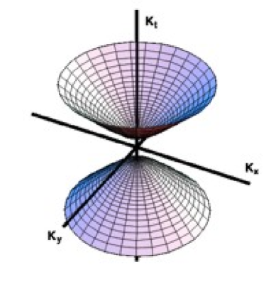
Figure 3: Hyperboloid of the parametric amplifier, the counterpart of the Poincaré sphere of the beam splitter shown in Fig. 2. The picture schematically illustrates the $K$ operators (6.21). Depending on the sign of the photon-number difference $\hat{K}_{z}+1/2$, the amplifier operates on the upper (positive) or the lower (negative) sheet of the hyperboloid. Amplification processes draw trajectories on one of the sheets, consisting of the Lorentz transformations (6.74).

Since $\hat{K}_{z}$ commutes with $\hat{K}_{t}$, $\hat{K}_{x}$ and $\hat{K}_{y}$, the $K$ operators generate transformations with the invariant (6.23), the quantum analog of the squared space-time distance [97] in 2+1 dimensions. In other words, the $K$ operators generate effective Lorentz transformations. In fact, we find

$$\exp(-i\Theta\hat{K}_{y})\left(\begin{array}[]{c}\hat{K}_{t}\\ \hat{K}_{x}\\ \hat{K}_{y}\end{array}\right)\exp(i\Theta\hat{K}_{y}) = \left(\begin{array}[]{ccc}\cosh\Theta&\sinh\Theta&0\\ \sinh\Theta&\cosh\Theta&0\\ 0&0&1\end{array}\right)\left(\begin{array}[]{c}\hat{K}_{t}\\ \hat{K}_{x}\\ \hat{K}_{y}\end{array}\right)\,,$$ (6.33)

$$\exp(-i\Omega\hat{K}_{x})\left(\begin{array}[]{c}\hat{K}_{t}\\ \hat{K}_{x}\\ \hat{K}_{y}\end{array}\right)\exp(i\Omega\hat{K}_{x}) = \left(\begin{array}[]{ccc}\cosh\Omega&0&-\sinh\Omega\\ 0&1&0\\ -\sinh\Omega&0&\cosh\Omega\end{array}\right)\left(\begin{array}[]{c}\hat{K}_{t}\\ \hat{K}_{x}\\ \hat{K}_{y}\end{array}\right)\,,$$ (6.43)

$$\exp(-i\Phi\hat{K}_{t})\left(\begin{array}[]{c}\hat{K}_{t}\\ \hat{K}_{x}\\ \hat{K}_{y}\end{array}\right)\exp(i\Phi\hat{K}_{t}) = \left(\begin{array}[]{ccc}1&0&0\\ 0&\cos\Phi&\sin\Phi\\ 0&-\sin\Phi&\cos\Phi\end{array}\right)\left(\begin{array}[]{c}\hat{K}_{t}\\ \hat{K}_{x}\\ \hat{K}_{y}\end{array}\right)\,,$$ (6.53)

two Lorentz transformations [97] with effective velocities $v_{x}/c=\tanh\Theta$ and $v_{y}/c=\tanh\Omega$ and one rotation with angle $\Phi$. We obtain for the mode operators

$$\exp(-i\Theta\hat{K}_{y})\left(\begin{array}[]{c}\hat{a}_{1}\\ \hat{a}_{2}^{\dagger}\end{array}\right)\exp(i\Theta\hat{K}_{y}) = \left(\begin{array}[]{cc}\cosh(\Theta/2)&\sinh(\Theta/2)\\ \sinh(\Theta/2)&\cosh(\Theta/2)\\ \end{array}\right)\left(\begin{array}[]{c}\hat{a}_{1}\\ \hat{a}_{2}^{\dagger}\end{array}\right)\,,$$ (6.60)

$$\exp(-i\Omega\hat{K}_{x})\left(\begin{array}[]{c}\hat{a}_{1}\\ \hat{a}_{2}^{\dagger}\end{array}\right)\exp(i\Omega\hat{K}_{x}) = \left(\begin{array}[]{cc}\cosh(\Omega/2)&i\sinh(\Omega/2)\\ -i\sinh(\Omega/2)&\cosh(\Omega/2)\\ \end{array}\right)\left(\begin{array}[]{c}\hat{a}_{1}\\ \hat{a}_{2}^{\dagger}\end{array}\right)\,,$$ (6.67)

$$\exp(-i\Phi\hat{K}_{t})\left(\begin{array}[]{c}\hat{a}_{1}\\ \hat{a}_{2}^{\dagger}\end{array}\right)\exp(i\Phi\hat{K}_{t}) = \left(\begin{array}[]{cc}e^{i\Phi/2}&0\\ 0&e^{-i\Phi/2}\\ \end{array}\right)\left(\begin{array}[]{c}\hat{a}_{1}\\ \hat{a}_{2}^{\dagger}\end{array}\right)\,,$$ (6.74)

These are all transformations that belong to the class (6.1). Therefore, parametric amplifiers generate effective Lorentz transformations. The measured quadrature-noise reduction [94] of $7\mbox{dB}$ ($20\%$) gives, according to Eq. (6.9), a $\Theta$ parameter of $-\log 0.2$, which corresponds to an effective velocity of $v/c=\tanh\Theta=0.92$. Finally, we employ the Lorentz generators (6.21) to represent the evolution operator of the parametric amplifier with the matrix (6.5). We use our results (6.74) and get

$$\hat{B}=\exp(-i\Phi\hat{K}_{t})\,\exp(-i\Theta\hat{K}_{y})\,\exp(-i\Psi\hat{K}_{t})\,\exp(-i\Lambda\hat{K}_{z})\,.$$ (6.75)

Passive optical instruments such as beam splitters preserve the total number of photons (3.7), they conserve energy. The parametric amplifier is subject to a conservation law as well. The generators of the evolution operator (6.75) commute with $\hat{K}_{z}$. Consequently, the photon-number difference is conserved,

$$\hat{a}_{1}^{\prime\dagger}\hat{a}_{1}^{\prime}-\hat{a}_{2}^{\prime\dagger}\hat{a}_{2}^{\prime}=\hat{a}_{1}^{\dagger}\hat{a}_{1}-\hat{a}_{2}^{\dagger}\hat{a}_{2}\,.$$ (6.76)

Photons are emitted in pairs, one in the signal and one in the idler beam, as we would expect from the Hamiltonian (3.33).

6.3 Quantum correlations

Conservation laws manifest themselves in correlations. For example, picture a pair of two particles with spin, say two polarized photons. The particles are produced at one spot and then they move away from each other. Suppose that the total spin of the two particles has been zero initially and that spin is conserved. Now, if we measure the spin of the first particle, the second one must have the opposite spin, regardless which type of polarization we are probing, linear or circular, and regardless how far apart the particles are. Such long-ranging correlations exist due to conservation laws, they do not violate the relativistic causality, because they do not cause each other, but rather have a cause in common, and they are completely classical. Quantum mechanics adds a subtlety, a decisive yet quantitatively subtle feature. For quantum particles the outcomes of the spin measurements may be probabilistic, depending on their state, but the spins of the partners are correlated. For example, consider the singlet state of two photons in two light beams, with two orthogonal polarization modes $(+)$ and $(-)$ each,

$$|\psi\rangle=\frac{1}{\sqrt{2}}\big{(}|+\rangle_{1}|-\rangle_{2}-\big{(}|-\rangle_{1}|+\rangle_{2}\big{)}\,,$$ (6.77)

or, written as Fock states,

$$|\psi\rangle=\frac{1}{\sqrt{2}}\big{(}|1\rangle_{1+}|1\rangle_{2-}-\big{(}|1\rangle_{1-}|1\rangle_{2+}\big{)}\,.$$ (6.78)

The polarization of photon 1 is completely random, $(+)$ or $(-)$ with 50% chance, but the polarization of the second photon is always correlated to the first one. The quantum state (6.77) is entangled — the vector $|\psi\rangle$ of the total state does not factorize into the state vectors of the subsystems. Now, suppose we measure the polarization of the first photon, with respect to a given axis, and we turn the polarizer of the second by an angle. In this case, the measurement results are not perfectly correlated anymore. However, we can quantify the correlation degree by calculating the difference $D$ between the statistical frequency of coincidences and the frequency of detecting the opposite spin, after many repeated runs of the experiment for each setting of the polarizer angle. Any spin measurement is characterized by the scalar product of a three-dimensional unity vector ${\bf a}$ with the vector of the Pauli matrices ${\bf\sigma}=(\sigma_{x},\sigma_{y},\sigma_{z})^{T}$ of Eq. (4.5), where ${\bf a}$ describes the polarizer setting on the Poincare sphere. We obtain for the singlet state (6.77)

$$D({\bf a}_{1},{\bf a}_{2})=\langle\psi\,|\,({\bf a}_{1}\cdot{\bf\sigma}_{1})\,({\bf a}_{2}\cdot{\bf\sigma}_{2})\,|\,\psi\rangle=-{\bf a}_{1}\cdot{\bf a}_{2}\,.$$ (6.79)

It turns out [19, 20] that $D$ violates certain inequalities for local hidden variables, based on classical statistics, called Bell’s inequalities after their discoverer [19]. Suppose that the particles are classical by nature, but are engaged in a quantum conspiracy. Before they are separated they agree on the outcome of spin measurements denoted in some hypothetical hidden variables that determine the measurement results. Although the observer is unaware of the plot, he can put constraints on the correlator, for example [45, 46]

$$D({\bf a}_{1},{\bf a}_{2})+D({\bf a}_{1},{\bf a}_{2}^{\prime})+D({\bf a}_{1}^{\prime},{\bf a}_{2})-D({\bf a}_{1}^{\prime},{\bf a}_{2}^{\prime})\leq 2\,,$$ (6.80)

assuming that the particles cannot communicate with each other after they have been separated. The spin correlations (6.79) of the quantum state (6.77) violate the Bell inequality (6.80) by maximally a factor of $\sqrt{2}$, as one may verify. Quantum particles can be slightly stronger correlated than classical statistics allows. Violations of Bell’s inequalities have been convincingly demonstrated in several experiments since the major breakthrough in efficiency due to Aspect [6], see e.g. Refs. [174, 190]. The parametric downconverter [127, 168] is the central tool in most modern tests of genuine quantum correlations. Apart from probing the foundations of quantum mechanics, quantum correlations are beginning to play a decisive role in tasks beyond the capabilities of classical physics such as quantum cryptography [39, 59] and in other forms of quantum communication [30, 135]. Parametric amplifiers are frequently applied in this wider field of entanglement engineering.

The debate on quantum correlations, on the “spooky action at a distance”, that preceded any applications of entanglement, dates back to the 1935 paper [51] “Can Quantum-Mechanical Description of Physical Reality Be Considered Complete” by Einstein, Podolsky and Rosen. Schrödinger [163] introduced the term entanglement to physics, Verschränkung, a German term used by cabinet makers for dovetailing, quite a fitting term for the quantum correlations in the natural world. The paper [51] by Einstein, Podolsky and Rosen has spawned a large literature [129] and has inspired a series of intriguing experiments, see for example Refs. [6, 28, 29, 30, 140, 141, 174, 190]. Interestingly, the parametric amplifier represents not only the device of choice for many modern applications of quantum correlations, but the amplifier is also able to reproduce the original argument by Einstein, Podolsky and Rosen for the quadratures $q$ and $p$ [158] in the experiment [140, 141].

Suppose the signal and idler modes are in the vacuum state initially. An optical parametric amplifier is just an amplifier after all. So, if the initial amplitude is zero the amplified amplitude remains zero. However, amplitude fluctuations get amplified. Remember the classic example of parametric resonance [96], the child on the playground swing where rocking at twice the frequency of the swing amplifies tiny initial movements. In the case of the optical parametric amplifier, the vacuum fluctuations are amplified. The resulting quantum state, called the two-mode squeezed vacuum, comes close to the original state considered by Einstein, Podolsky and Rosen in their 1935 paper [51]. We calculate its Wigner function. Initially, the two modes are in the vacuum state with the Wigner function [110]

$$W(q_{1},p_{1},q_{2},p_{2})=\frac{1}{\pi^{2}}\,\exp\left(-q_{1}^{2}-p_{1}^{2}-q_{2}^{2}-p_{2}^{2}\right)\,.$$ (6.81)

We recall that simple optical instruments transform the Wigner function as if $W$ were a classical probability distribution of the quadratures. For simplicity, we assume that the $\underline{S}$ matrix (6.2) of the amplifier is the real matrix (3.30). We obtain from the transformation rule (3.40) the Wigner function of the two-mode squeezed vacuum

$$W^{\prime}(q_{1},p_{1},q_{2},p_{2})=\frac{1}{\pi^{2}}\,\exp\left(-q_{1}^{\prime 2}-p_{1}^{\prime 2}-q_{2}^{\prime 2}-p_{2}^{\prime 2}\right)$$ (6.82)

with

$$\left(\begin{array}[]{c}q_{1}^{\prime}\\ q_{2}^{\prime}\end{array}\right) = \left(\begin{array}[]{cc}\cosh\zeta&\sinh\zeta\\ \sinh\zeta&\cosh\zeta\end{array}\right)\left(\begin{array}[]{c}q_{1}\\ q_{2}\end{array}\right)\,,$$ (6.89)

$$\left(\begin{array}[]{c}p_{1}^{\prime}\\ p_{2}^{\prime}\end{array}\right) = \left(\begin{array}[]{cc}\cosh\zeta&-\sinh\zeta\\ -\sinh\zeta&\cosh\zeta\end{array}\right)\left(\begin{array}[]{c}p_{1}\\ p_{2}\end{array}\right)\,.$$ (6.96)

Consequently,

$$W^{\prime}=\frac{1}{\pi^{2}}\,\exp\left[-\frac{(q_{1}-q_{2})^{2}}{2e^{-2\zeta}}-\frac{(q_{1}+q_{2})^{2}}{2e^{2\zeta}}-\frac{(p_{1}+p_{2})^{2}}{2e^{-2\zeta}}-\frac{(p_{1}-p_{2})^{2}}{2e^{2\zeta}}\right]\,.$$ (6.97)

The Wigner function (6.97) indicates strong quadrature correlations when $|\zeta|$ is large. Suppose we measure the $q$ quadrature of the first beam using homodyne detection [110] and we find the value $q_{1}$. In this case a quadrature measurement of the second beam, some distance away from the first one, gives with high probability $q_{1}$ as well. The first measurement has prepared the second beam in a state that closely resembles a $q$ quadrature eigenstate. Now, if we measure the $p$ quadratures, with the result $p_{1}$ for the first beam, the second mode produces $-p_{1}$ with high probability. The $q$ and $p$ eigenstates cannot coexist, because of the canonical commutation relations (2.11). Therefore, depending on the measurements on the first beam, the second one is prepared in states that are mutually incompatible and that cannot coexist as “elements of reality” [51]. Of course, Einstein, Podolsky and Rosen did not mention quantum-optical quadratures in their paper [51], but rather position and momentum in real space, yet this does not fundamentally alter the argument. However, a hypothetical quantum conspiracy could explain the behavior Einstein, Podolsky and Rosen found so puzzling. The light beams could have originally agreed on with which probability they are going to produce all linear combinations of $q$ and $p$ quadratures. The Wigner function (6.97) reveals the plot. The function plays the role of the non-negative probability distribution for some hidden variables triggering all quadrature detection results. In our case, the quadratures themselves are the hidden variables $q_{1}$, $q_{2}$, $p_{1}$ and $p_{2}$. Ironically, the paradox that led to quantitative measures of quantum nonlocality can be explained classically. It would take a negative Wigner function [107] to violate Bell’s inequalities in quadrature space, as Bell has pointed out [21], although with flawed mathematics in his counterexample [82]. However, the two-mode squeezed vacuum state may well violate Bell’s inequalities for other observables than the quadratures [8], because the quasiprobability distributions in other variables [108, 109, 182] may be negative.

The parametric amplifier generates strong quantum correlations between the emerging light beams. In fact, one can argue [13, 14] that the correlations are the strongest possible for two equal oscillator modes with given average energy. To understand why, we calculate the reduced Wigner function of any of the modes, say mode 1. We obtain after Gaussian integration

$$\int_{-\infty}^{+\infty}\int_{-\infty}^{+\infty}W^{\prime}(q_{1},p_{1},q_{2},p_{2})\,\mathrm{d}q_{2}\,\mathrm{d}p_{2}=W_{\mathrm{th}}(q_{1},p_{1})\,,$$ (6.98)

where $W_{\mathrm{th}}$ denotes the Wigner function (5.7) of the thermal state (5.8) with the temperature

$$T=\frac{\hbar\omega}{2k_{\mathrm{B}}\ln\coth\zeta}\,.$$ (6.99)

The reduced Wigner function describes the reduced quantum state of one of the correlated modes, averaged over the second mode. As we know from statistical physics [99], the thermal state is the state of maximal entropy with given energy, in the canonical Gibbs ensemble, the state of maximal disorder and minimal information. On the other hand, the total two-mode squeezed vacuum is a pure state. Consequently, this state stretches mostly across the correlations between the two entangled modes. When reduced to one mode, the subsystem contains as little information as possible. Therefore, the two-mode squeezed vacuum is indeed the most strongly correlated quantum states of two equal harmonic oscillators with given energy [13, 14]. The higher this energy the higher is the effective temperature (6.99) and the stronger are the quantum correlations.

Since the parametric amplifier conserves the photon-number difference (6.76) between signal and idler, the quantum correlations of the two-mode squeezed vacuum are particularly transparent in terms of photon-number states, i.e. in the Fock representation. We utilize the disentangling theorem [58, 147]

$$\exp(2i\zeta\hat{K}_{y})=\exp(\hat{a}_{1}^{\dagger}\hat{a}_{2}^{\dagger}\tanh\zeta)\,\exp(-2\hat{K}_{t}\ln\cosh\zeta)\,\exp(-\hat{a}_{1}\hat{a}_{2}\tanh\zeta)\,,$$ (6.100)

and get for the two-mode squeezed vacuum state

$$|\psi\rangle=\exp(2i\zeta\hat{K}_{y})\,|0\rangle_{1}|0\rangle_{2} = \exp(\hat{a}_{1}^{\dagger}\hat{a}_{2}^{\dagger}\tanh\zeta)\,\exp(-2\hat{K}_{t}\ln\cosh\zeta)\,|0\rangle_{1}|0\rangle_{2}$$ (6.101)

$$= \frac{1}{\cosh\zeta}\sum_{n=0}^{\infty}\frac{1}{n!}\,(\hat{a}_{1}^{\dagger}\hat{a}_{2}^{\dagger}\tanh\zeta)^{n}\,|0\rangle_{1}|0\rangle_{2}$$

$$= \frac{1}{\cosh\zeta}\sum_{n=0}^{\infty}(\tanh\zeta)^{n}\,|n\rangle_{1}|n\rangle_{2}\,.$$

We see that $|\psi\rangle$ consists entirely of photon pairs $|n\rangle_{1}|n\rangle_{2}$. We also see that the reduced density operator $\mathrm{tr}_{2}\{|\psi\rangle\langle\psi|\}$ is indeed the thermal state (5.8) with temperature (6.99). In spontaneous parametric downconversion [127] the squeezing parameter $\zeta$ is small. In this regime, $\zeta^{2}$ gives the probability for producing a single pair of photons, as we see from a first-order perturbation theory with the Hamiltonian (3.33), and $\zeta^{2n}$ gives the probability for $n$ independently produced pairs. So, according to the result (6.101), the two-mode squeezed vacuum seems to consist of indistinguishable photon pairs, in the regime of weak amplification. Spontaneous downconversion [127] has been frequently used for generating single pairs of photons, because the probability for multiple pairs is very low, $\zeta^{2n}$ compared with $\zeta^{2}$. High-efficiency single-photodetectors operate like Geiger counters, where a single photon triggers an electron-hole avalanche [110]. Since the initial photons are just triggers, the detectors cannot discriminate between one or more detected photons in each detection click. Therefore, it is an experimental advantage to guarantee that mostly single pairs occur, which of course limits the rate of pair production.

The interference experiments with single photons mentioned in Sec. 4.3 have been performed with photon pairs generated in spontaneous parametric downconversion [127]. Here the quantum state (6.101) of light is essentially

$$|\psi\rangle\approx|0\rangle_{1}|0\rangle_{2}+\zeta\,|1\rangle_{1}|1\rangle_{2}\,.$$ (6.102)

In such experiments only those experimental runs count where photons are counted, the time when the detectors are not firing is ignored, which reduces the quantum state to the photon pair $|1\rangle_{1}|1\rangle_{2}$. Postselection disentangles the two-mode squeezed vacuum. We argued in Sec. 4.3 that the interference of the photon pair $|1\rangle_{1}|1\rangle_{2}$ at a 50:50 beam splitter generates the entangled state (4.86). Without postselection, however, this state is the disentangled product of two single-mode squeezed vacua, as we see from the factorization (6.6) of the $\underline{S}$ matrix. The notion of entanglement is to some extent relative.

Finally, we explain briefly how the singlet state (6.78) is generated in spontaneous parametric downconversion [127]. The spin singlet (6.78) refers to the polarization state of two light beams with two polarization modes each, four modes in total with the mode operators $\hat{a}_{1+}$, $\hat{a}_{1-}$, $\hat{a}_{2+}$ and $\hat{a}_{2-}$. The singlet is completely unpolarized, but contains polarization correlations, Bell correlations [20] in fact. Therefore, the creation process of the singlet must be polarization invariant. The Hamiltonian of parametric downconversion is quadratic in the mode operators of signal and idler, as long as the pump can be regarded as a classical parameter. Consequently, we need a quadratic form of the annihilation operators $\hat{a}_{1+}$, $\hat{a}_{1-}$, $\hat{a}_{2+}$ and $\hat{a}_{2-}$ that is invariant under polarization transformations [101]. The rotations on the Poincare sphere (4.49) correspond to the mode transformations (4.70) of the beam-splitter type (4.1) of the polarization modes $(\hat{a}_{1+},\hat{a}_{1-})^{T}$ and $(\hat{a}_{2+},\hat{a}_{2-})^{T}$, with identical SU(2) matrices [48]. Written in matrix form

$$\underline{\hat{a}}^{\prime}=\underline{B}\,\underline{\hat{a}}\,,\quad\underline{\hat{a}}=\left(\begin{array}[]{cc}\hat{a}_{1+}&\hat{a}_{2+}\\ \hat{a}_{1-}&\hat{a}_{2-}\end{array}\right)\,,\quad\underline{B}^{-1}=\underline{B}^{\dagger}\,,\quad\mathrm{det}\underline{B}=1\,.$$ (6.103)

The determinant of the $\underline{\hat{a}}$ matrix has the desired property, because $\mathrm{det}\underline{\hat{a}}^{\prime}=\mathrm{det}\underline{B}\,\mathrm{det}\underline{\hat{a}}$. Consequently, we arrive at the effective Hamiltonian

$$\hat{H}=ie^{i\varphi}\zeta\,\mathrm{det}\underline{\hat{a}}^{\dagger}-ie^{-i\varphi}\zeta\,\mathrm{det}\underline{\hat{a}}$$ (6.104)

with real squeezing parameter $\zeta$ and real phase $\varphi$. We assume that both signal and idler have initially been in the vacuum state. We use the result (6.101) and get

$$|\psi\rangle = \exp(-i\hat{H})\,|0\rangle_{1+}|0\rangle_{1-}|0\rangle_{2+}|0\rangle_{2+}=|\psi\rangle_{+}+|\psi\rangle_{-}\,,$$

$$|\psi\rangle_{\pm} = \frac{1}{\cosh\zeta}\sum_{n=0}^{\infty}\left(\pm e^{-i\varphi}\tanh\zeta\right)^{n}\,|n\rangle_{1\pm}|n\rangle_{2\mp}\,,$$ (6.105)

which, after postselecting for single photon pairs, gives the Bell state (6.78) in the regime of spontaneous parametric downconversion. We describe briefly how the downconverter can realize the Hamiltonian (6.104).

Figure 4: Schematic of the downconversion process (with type-II phase matching). An ultraviolet photon incident on a nonlinear crystal can sometimes spontaneously split into two correlated infrared photons. These photons are emitted on opposite sides of the pump beam, along two cones, one of which has horizontal polarization, the other of which has vertical polarization. Photon pairs emitted along the intersections of the cones are entangled in polarization — each photon is individually unpolarized, and yet the photons necessarily have perpendicular polarizations, no matter how far apart they are. (Courtesy of Paul Kwiat.)

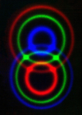
Figure 5: Entangled light. Colorized infrared photograph of the measured downconversion output [91] schematically shown in Fig. 4. The green rings correspond to photons with roughly equal energies (half that of the parent pump photon). Where the rings intersect the polarization state of the light is entangled. (Courtesy of Anton Zeilinger, Institut für Experimentalphysik, Universität Wien.)

Downconversion is a nonlinear optical process [26, 168] where a pump beam $E_{p}$ of frequency $\omega_{p}$ generates two waves, the signal $E_{s}$ and the idler $E_{i}$, of frequencies $\omega_{s}$ and $\omega_{i}$ with $\omega_{p}=\omega_{s}+\omega_{i}$. This three-wave mixing [168] requires an appropriately anisotropic medium, a crystal, because the interaction Hamiltonian of the three fields $\chi^{(2)}E_{p}E_{s}E_{i}$ is not invariant under parity transformations where the fields change sign. In an anisotropic medium light propagates as ordinary or as extraordinary waves with opposite polarizations [27]. There are two principal types of downconverters. In type I [168] the modes $E_{s}$ and $E_{i}$ are both ordinary or extraordinary waves. In type II downconversion [168] either $E_{s}$ or $E_{i}$ is ordinary and the other wave is extraordinary, and hence the two have opposite polarizations. The downconverted light leaves the crystal in two cones that display the conservation laws involved — the conservation of energy, $\omega_{p}=\omega_{s}+\omega_{i}$, and the conservation of the wave vectors (phase matching condition [168]), see Fig. 4. Where the cones intersect the polarization state is undecided. According to our theory, this polarization-invariant state of light is the state (6.105). The two intersection lines of the emerging light cones carry polarization Bell states [91], see Fig. 5. Alternatively, one can employ two subsequent type I crystals with orthogonal optical axes [92]. The crystals downconvert pump light into entangled beams in all directions. All this shows that the parametric amplifier is a superb device for generating quantum correlations of light.

7 Optical black hole

Black holes are optical instruments as well, although they tend to operate on grander scales than ordinary laboratory equipment. First of all, black holes are gravitational lenses [162] — the gravitational fields surrounding them focus light from other sources and may cause a multitude of optical illusions. Black holes share this feature with other gravitating bodies such as entire galaxies, stars or even individual planets. The distinctive feature of a black hole is the event horizon [131]. The horizon, surrounding the hole, is a place of no return. Beyond the horizon, everything falls into the hole, no matter how fast it moves, even light. Here gravity has tilted the future light cones such that they all point inwards, see Fig. 6.

Figure 6: Black hole. Gravity modifies the metric of space and time. In flat space, far away from the gravitating object, the light cones stand upright in a space-time diagram. Gravity is tilting the light cones, bending light. At the event horizon all future light cones point inwards. Light cannot escape anymore, and so cannot anything else. (Picture by Enrique Arilla.)

As we discuss in this section, the horizon turns the black hole into an active optical instrument. The hole does not merely act as a gravitational lens, it emits radiation as well, Hawking radiation [25, 36, 67, 68]. The hole appears as a thermal black body with a temperature that depends on the gravity at the horizon (and hence [131] on the horizon’s area and the hole’s mass). The characteristic wavelength at the peak of the Planck spectrum is comparable to the radius of the horizon [25, 36], more than $1\mbox{km}$ for the known solar-mass or larger black holes, which makes Hawking radiation far too cold to be observable against the cosmic microwave background of about $1\mbox{mm}$ wavelength.

On the other hand, since black holes are optical instruments after all, why not use optical equipment to make one? Such table-top black holes would be much smaller than the astronomical ones. Since the scale of the hole determines the temperature of the Hawking radiation, one would expect them to radiate stronger than their larger archetypes in space. Most of the proposed artificial black holes [136] are based on a simple idea [181, 184]: Consider a moving medium with spatially varying flow speed, say water going down the drain of a bathtub. Waves in the fluid, sound waves [181, 184], surface waves [165] or light waves [34, 111, 164] are trapped when the flow exceeds the speed of the wave in the medium, the speed of sound or the effective speed of light, for example. To turn this simple analogy into measurements of emergent Hawking radiation will take extraordinary media though — Bose-Einstein condensates of alkali vapours [49, 154] for sonic holes [55, 117], two phases of superfluid Helium-3 [186] for ripple holes [165] and slow-light media [116, 125] for optical holes [112, 114, 115]. Note that the possibly realistic version of the optical hole [114, 115] differs from ordinary black holes. It does not involve a moving medium and belongs to a different class of quantum catastrophes [115] than the Hawking effect [25, 36, 67, 68]. Much in this field is still in flux and is connected to other areas of physics outside of the scope of this article. Here we discuss an optical Gedankenexperiment, not a realistic proposal, to show how Hawking radiation emerges in principle.

7.1 Light in moving media

Consider a dielectric medium with an incredibly strong electric permittivity $\varepsilon\gg 1$ and with unity magnetic permeability, for simplicity. Such a medium would significantly reduce the phase velocity of light, $c^{\prime}$, because

$$c^{\prime 2}=\frac{c^{2}}{\varepsilon}\,.$$ (7.1)

Note that the slow light [116, 125] demonstrated in recent experiments [66, 121, 153] represents a different case where the group velocity of light is reduced and not the phase velocity. Consider for simplicity a one-dimensional medium moving with the spatially varying flow speed $u(x)$. The Lagrangian of the electromagnetic field is the Lorentz scalar [97, 113]

$${\mathscr{L}}=\frac{1}{2}\left(ED-BH\right)\,.$$ (7.2)

At any place in the moving medium we can imagine a co-moving frame of coordinates where the medium is at rest, denoted by primes. The Lagrangian is invariant,

$${\mathscr{L}}=\frac{1}{2}\left(E^{\prime}D^{\prime}-B^{\prime}H^{\prime}\right)\,.$$ (7.3)

In a local co-moving frame, the $D^{\prime}$ and $H^{\prime}$ fields are connected to the $E^{\prime}$ and $B^{\prime}$ fields via the constitutive equations [74, 100]

$$D^{\prime}=\varepsilon_{0}\varepsilon E^{\prime},\quad H^{\prime}=\varepsilon_{0}c^{2}B^{\prime}\,.$$ (7.4)

We represent the $E^{\prime}$ and $B^{\prime}$ fields in terms (2.2) of the vector potential $A$, a scalar in 1+1 dimensions. For non-relativistic velocities of both the medium and the light we obtain from the local Galilei transformations to the laboratory frame

$$\partial_{t}^{\prime}=\partial_{t}+u\partial_{x},\quad\partial_{x}^{\prime}=\partial_{x}\,.$$ (7.5)

In this way we arrive at the Lagrangian in the laboratory frame

$${\mathscr{L}}=\frac{\varepsilon_{0}\varepsilon}{2}\Big{(}(\partial_{t}A)^{2}+2u(\partial_{t}A)(\partial_{x}A)+(u^{2}-c^{\prime 2})(\partial_{x}A)^{2}\Big{)}$$ (7.6)

that generates the Euler-Lagrange equation [97]

$$\partial_{t}\varepsilon(\partial_{t}+u\partial_{x})A+\partial_{x}\varepsilon[u\partial_{t}+(u^{2}-c^{\prime 2})]\partial_{x}A=0\,.$$ (7.7)

This wave equation describes the propagation of classical light in moving media in one spatial dimension.

7.2 Space-time geometry

Remarkably, light turns out to experience the moving medium as an emergent space-time geometry [62, 111, 113, 137, 151, 152]. To understand why, consider the simplest case, our one-dimensional medium with large $\varepsilon$. We introduce the relativistic notation

$$x^{0}=t,\quad x^{1}=x,\quad\partial_{0}=\partial_{t},\quad\partial_{1}=\partial_{x}$$ (7.8)

and adopt Einstein’s summation convention over repeated indices. In this way we write the Lagrangian (7.6) as

$${\mathscr{L}}=\frac{\varepsilon_{0}}{2}\,f^{\mu\nu}(\partial_{\mu}A)(\partial_{\nu}A)$$ (7.9)

in terms of the matrix

$$f^{\mu\nu}=\varepsilon\left(\begin{array}[]{cc}1&u\\ u&-c^{\prime 2}+u^{2}\end{array}\right)\,,$$ (7.10)

which gives the Euler-Lagrange equation

$$\partial_{\mu}f^{\mu\nu}\partial_{\nu}A=0\,.$$ (7.11)

Suppose that $\varepsilon$ is constant while $u$ may vary in space. We introduce the metric

$$g_{\mu\nu}=\left(\begin{array}[]{cc}c^{\prime 2}-u^{2}&u\\ u&-1\end{array}\right)$$ (7.12)

with the determinant [97]

$$g=-c^{\prime 2}$$ (7.13)

and the inverse

$$g^{\mu\nu}=\frac{1}{c^{\prime 2}}\left(\begin{array}[]{cc}1&u\\ u&-c^{\prime 2}+u^{2}\end{array}\right)\,.$$ (7.14)

As long as $\varepsilon$ remains constant we can write the wave equation (7.11) as [97]

$$0=\frac{1}{\sqrt{-g}}\,\partial_{\mu}\sqrt{-g}\,g^{\mu\nu}\partial_{\nu}A=D_{\mu}D^{\mu}A\,.$$ (7.15)

The $D_{\mu}$ denote the covariant derivatives and $D_{\mu}D^{\mu}$ gives the D’Alembert operator in general coordinates with the metric (7.12). Equation (7.15) describes a mass-less field, light, in general relativity. Therefore, the electromagnetic field perceives the moving medium as the space-time geometry (7.12). Light-rays follow zero-geodesic lines measured with respect to the metric (7.12) [111]. In the history of optics, the oldest known paradigm of geometric guidance is Fermat’s Principle [27]: Light rays follow the shortest optical paths where the path length is measured with respect to the refractive index.

A dielectric medium acts on light, in focusing or scattering light, but, according to the principle of actio et reactio, light also acts on the medium, in exerting optical forces. We have ignored these forces here, assuming that the medium is very heavy. The light forces turn out to follow geometric ideas, too. The medium perceives the electromagnetic field as a space-time geometry as well. Light and dielectric matter see each other as geometries [113].

Finally, the idea that media modify the geometry of space and time can be turned around, at least speculatively. Can one interpret space-time curvature, i.e. gravity, as generated by a hypothetical fluid, as an emergent phenomenon in condensed-matter physics [186]? Sir Isaac Newton speculated in 1675 [35] that gravity acts through “an aetherial medium, much of the same constitution with air, only the vibrations far more swift and minute”, one of Sir Isaac’s departures to hypotheses. Much later, in 1968, Andrei Sakharov, father of the Soviet hydrogen bomb, dissident and Nobel Peace Price laureate, noticed [160] that Einstein’s general relativity could appear as the effect of fluctuations of the quantum vacuum, the modern form of the aether.

7.3 Horizon

The effective metric of light in moving media [62, 113] does not cover all possible space-time manifolds, but the generated geometries are rich enough to include horizons. The horizon is the place where the flow speed $u$ exceeds the speed of light in the medium, $c^{\prime}$. Here, according to the metric (7.12), the measure of time, $c^{\prime 2}-u^{2}$, is zero — time appears to stand still. Light propagating against the current freezes. In fact, black holes have been termed “frozen stars” [65]. Immediately before the horizon, any outgoing light struggles to escape. The closer the distance to the horizon, the more optical cycles it takes to move forward. In turn, the wave length of light shrinks to zero at the horizon. On the other side of the horizon, no counter-propagating light is able to escape anymore.

Let us turn these words into formulae. Assume for simplicity that $\varepsilon$ is constant. In this case the general solution of the wave equation (7.11) is

$$A(x,t)=A_{+}(\tau_{+})+A_{-}(\tau_{-})\,,\quad\tau_{\pm}=t-\int\frac{\mathrm{d}x}{u\pm c^{\prime}}\,.$$ (7.16)

Note that also the complex conjugate, $A^{*}$, is a solution, because the wave equation (7.11) is real. Suppose, without loss of generality, that the medium flows from the right to the left such that $u$ is negative. Hence $A_{+}(\tau_{+})$ describes counter-propagating and $A_{-}(\tau_{-})$ co-propagating wavepackets. The $\tau_{\pm}$ are the null coordinates in the global medium frame. (Note that in more than one spatial dimension such a frame does not exist in general.) Assume that the velocity $u$ exceeds the effective speed of light at one point, say $x=0$, such that

$$u\sim-c^{\prime}+\alpha x\quad\mbox{near}\,\,x=0\,.$$ (7.17)

The positive constant $\alpha$ describes the velocity gradient at the horizon, the analogue of the surface gravity at the event horizon of a gravitational hole. In the vicinity of the horizon we get

$$\tau_{+}\sim t-\frac{\ln(x/x_{\pm\infty})}{\alpha}$$ (7.18)

with the integration constants $x_{\pm\infty}$. Therefore, to escape from the horizon takes an exponentially long time. Assuming monochromatic light, where $A_{+}=\exp(-i\omega\tau_{+})$, we see that the phase $\varphi$ of the light wave is logarithmic in $x/x_{\infty}$. Consequently, the wavelength $2\pi/(\partial_{x}\varphi)$ is indeed proportional to the distance from the horizon,

$$\lambda\sim\lambda_{\infty}\frac{x}{x_{\infty}}\,.$$ (7.19)

We also see that the $\tau_{+}$ coordinate distinguishes the left and the right side of the horizon. The constants $x_{\pm\infty}$ must be positive on the right and negative on the left side, for not running into problems with complex time. The horizon cuts space into two disconnected parts.

7.4 Hawking radiation

Consider the quantum theory of light for our artificial black hole, the moving medium. As usual [25, 191], the quantum field $\hat{A}$ consists of a set of modes with the mode functions $A_{k}$ and the Bose annihilation operators $\hat{a}_{k}$, see Eq.  (2.6). In the moving medium, the mode functions are subject to the wave equation (7.11). The modes are normalized according to a scalar product that ought to stay invariant in time and that should approach the scalar product (2.4) in the limiting case when the medium is at rest. We put

$$\left(A_{1},A_{2}\right) \equiv \frac{i\varepsilon_{0}}{\hbar}\int\left(A_{1}^{*}\,f^{0\nu}\partial_{\nu}\,A_{2}-A_{2}\,f^{0\nu}\partial_{\nu}\,A_{1}^{*}\right)\mathrm{d}x$$ (7.20)

$$= \frac{i\varepsilon_{0}}{\hbar}\int\Big{(}A_{1}^{*}\,(\partial_{t}+u\partial_{x})A_{2}-A_{2}\,(\partial_{t}+u\partial_{x})A_{1}^{*}\Big{)}\,\varepsilon\,\mathrm{d}x\,.$$

The scalar product (7.20) is the desired one, because it agrees with Eq.  (2.4) when $u$ vanishes and the product is indeed a constant in time, because of the conservation law

$$\partial_{\mu}\left(A_{1}^{*}\,f^{\mu\nu}\partial_{\nu}A_{2}-A_{2}\,f^{\mu\nu}\partial_{\nu}A_{1}^{*}\right)=0\,.$$ (7.21)

After these general remarks on quantum light in moving media we return to the optical black hole.

Consider the monochromatic modes with frequency $\omega$ that are propagating against the current, the mode function $A_{R}$ on the right side of the horizon and the function $A_{L}$ on the left side,

$$A_{R}={\cal A}_{R}\,\Theta(x)\,\exp(-i\omega\tau_{+})\,,\quad A_{L}={\cal A}_{L}\,\Theta(-x)\,\exp(i\omega\tau_{+})\,.$$ (7.22)

The unity step functions $\Theta(\pm x)$ indicate that $A_{R}$ is only supported on the right side, whereas $A_{L}$ exists solely on the left side. Note that the mode $A_{L}$ on the left side beyond the horizon oscillates with the negative frequency $-\omega$, in order to represent a proper positive-norm mode (2.7). In fact, we see from

$$i(\partial_{t}+u\partial_{x})A_{L}=-\omega\,\frac{c^{\prime}}{u+c^{\prime}}\,A_{L}$$ (7.23)

that the normalization integral (7.20) is positive for negative $u+c^{\prime}$, as is the case beyond the horizon. Negative frequencies $\omega$ correspond to negative energies $\hbar\omega$. Consequently, the artificial black hole does not have a natural ground state, at least in our simplified model where the permittivity $\varepsilon$ and the flow $u$ are given and fixed, ignoring the backaction of the light onto the medium. The vacuum state, the state of zero photons, traditionally the ground state, may thus depend on the history of the horizon, on the catastrophic event creating the black hole. In space, the gravitational collapse creates the black hole. In our laboratory analogue, the medium must have been accelerated in the past to form a stationary flow with a horizon. Consider the quantum theory of light in the Heisenberg picture where the field operators evolve and the quantum state of light remains constant. Trace the mode functions back into their pre-horizon history, in order to find the decisive signature of the modes that distinguishes the initial quantum vacuum, and hence the final vacuum, too. Complex analysis provides us with elegant theoretical tools for this purpose [36, 50].

Before the horizon has been formed, the vacuum modes stretched over the entire medium. Counter-propagating waves consisted of superpositions of plane waves with positive wavenumbers,

$$A_{0}(x,t)\sim\int_{0}^{+\infty}\widetilde{A}_{0}(k)\,\exp(ikx-i\omega t)\,\mathrm{d}k\,,\quad t\rightarrow-\infty\,.$$ (7.24)

Consider the analytic continuation of the vacuum modes to complex $x$ values. The $A_{0}$ are analytic on the upper half plane, because here $\exp(ikx)$ decays for positive wavenumbers $k$, such that $A_{0}$ cannot develop singularities. Now, imagine that the original modes evolve during the formation of the horizon where the medium is gently accelerated to exceed the effective speed of light beyond one point. A smooth process cannot fundamentally alter the analytic properties of waves. Consequently, we can employ the analyticity of the mode functions as a marker to distinguish the vacuum state of light. The modes $A_{R}$ and $A_{L}$ are clearly non-analytic, because they lack support on either one of the horizon sides. Yet we can glue $A_{R}$ and $A_{L}^{*}$ together to form analytic wave functions [36]. Close to the horizon, we have

$$\exp(-i\omega\tau_{+})\sim(x/x_{+\infty})^{i\omega/\alpha}\exp(-i\omega t)\,.$$ (7.25)

Circumventing the horizon on the upper half plane, we use the property $(-z)^{i\mu}=e^{-\pi\mu}z^{i\mu}$, and find the combinations

$$A_{1}=A_{R}\cosh\zeta+A_{L}^{*}\sinh\zeta\,,\quad A_{2}=A_{R}^{*}\sinh\zeta+A_{L}\cosh\zeta$$ (7.26)

that are analytic on the upper half plane when

$$\tanh\zeta=e^{-\pi\omega/\alpha}\,.$$ (7.27)

The vacuum modes $A_{1}$ and $A_{2}$ are normalized according to Eq. (2.7) with the scalar product (7.20), taking into account that both $A_{R}$ and $A_{L}$ are normalized and orthogonal, and that the norm of $A^{*}$ is the negative norm of $A$. The mode transformations (7.26) imply that

$$\left(\begin{array}[]{c}\hat{a}_{R}\\ \hat{a}_{L}^{\dagger}\end{array}\right)=\left(\begin{array}[]{cc}\cosh\zeta&-\sinh\zeta\\ -\sinh\zeta&\cosh\zeta\end{array}\right)\left(\begin{array}[]{c}\hat{a}_{1}\\ \hat{a}_{2}^{\dagger}\end{array}\right)\,.$$ (7.28)

The black hole acts as a parametric amplifier, transforming the incident vacuum into the two-mode squeezed vacuum state (6.101), the entangled Einstein-Podolsky-Rosen state [51]. The steeper the velocity gradient $\alpha$ the stronger is the entanglement and hence the energy of the two-mode squeezed vacuum. The horizon generates photon pairs, both propagating against the current, but one escaping on the right side of the horizon and the other drifting to the left. Somehow the flow must provide the energy for the photon production that, in turn, will cause friction. In space [131], the gravitational field surrounding the black hole, created by the mass of the collapsed object, should provide the energy for the emerging Hawking radiation. The black hole is evaporating and is getting smaller. All black holes are similar, apart from their scales [131]. Therefore, smaller holes generate larger gradients of the gravitational potential. Consequently [67], the evaporation is accelerating, until the black hole explodes in a grand fiery finale.

If we confine ourselves to the right side of the horizon, our natural place in the case of gravitational black holes, we perceive the two-mode squeezed vacuum (6.101) as the thermal state (5.8) with the temperature (6.99), the Hawking temperature

$$T=\frac{\hbar\alpha}{2\pi k_{\mathrm{B}}}\,.$$ (7.29)

The temperature depends only on the velocity gradient $\alpha$, the analogue of the surface gravity of the hole. Consequently, the Hawking temperature (7.29) is the same for the entire spectrum, which is highly non-trivial. The black hole appears as a black-body radiator in thermal equilibrium [17, 18, 36, 75], a mysterious result [67].

7.5 Grey-body factor

We have shown that the black hole acts as an active optical instruments, as a parametric amplifier. So far, we have ignored the passive optical properties of the hole, the analogue of the gravitational lens [162]. Here we sketch how these properties are taken into account, i.e., how to include the light scattering of the optical black hole. In our simple one-dimensional example, scattering occurs only when the permittivity $\varepsilon$ of the medium varies in space, because the solution (7.16) for constant $\varepsilon$ maintains co- and counter-propagating light as the separate waves $A_{+}(\tau_{+})$ and $A_{-}(\tau_{-})$. When $\varepsilon$ varies, we represent the monochromatic modes on the two sides of the horizon as

$$A_{R} = A_{+R}\exp({-i\omega\tau_{+}})+A_{-k}\exp({-i\omega\tau_{-}})\,,$$

$$A_{L} = A_{+L}\exp({+i\omega\tau_{+}})+A_{-k}\exp({-i\omega\tau_{-}})\,,$$ (7.30)

where the $A_{+R}$, $A_{+L}$ and $A_{-k}$ are slowly varying functions of $x$. Similar to Sec. 2.3, we construct the transfer matrix (2.16) in order to connect $A_{+R}$ and $A_{-k}$ between the various points on the right side of the horizon. Also in the case of moving media, the transfer matrix exhibits the structure (2.17) with the determinant (2.18). The latter property is a consequence of the conservation law (7.21) that implies for monochromatic modes

$$\partial_{x}\Big{(}i(\varepsilon u^{2}-c^{2})(A^{*}\,\partial_{x}A-A\,\partial_{x}A^{*})+2\omega\varepsilon u\,|A|^{2}\Big{)}=0\,.$$ (7.31)

Substituting the structure (7.30) with the transfer-matrix connection (2.16) gives the differential equation for the determinant (2.18).

Similar to Sec. 2.4, we use the transfer matrix to define the in and out modes, but starting here with the outgoing modes,

$$A_{R}^{\mathrm{out}}=u_{R}(x)\,e^{-i\omega t}\,,\quad A_{D}^{\mathrm{out}}=u_{D}(x)\,e^{-i\omega t}\,,$$ (7.32)

where $A_{R}^{\mathrm{out}}$ describes an outgoing counter-propagating wave, whereas $A_{D}^{\mathrm{out}}$ refers to a co-propagating wave. The $A_{R}^{\mathrm{out}}$ wave originates at the horizon, propagating to the right, whereas $A_{D}^{\mathrm{out}}$ propagates to the left at $+\infty$ and crosses the horizon without anything unusual happening. We assume that at $+\infty$ the effective speed of light, $c^{\prime}$ and the flow $u$ approach constants such that light approaches plane waves with the wavenumbers

$$k_{R}=\frac{\omega}{c^{\prime}(+\infty)+u(+\infty)}\,,\quad k_{D}=\frac{\omega}{c^{\prime}(+\infty)-u(+\infty)}\,.$$ (7.33)

In this case $u_{R}$ obeys the asymptotics

$$u_{R}(x)\sim{\cal A}_{R}\left\{\begin{array}[]{r@{\quad:\quad}l}(x/x_{+\infty})^{i\omega/\alpha}&x\rightarrow+0\\ a^{*}\,e^{ik_{R}x}+b^{*}\,e^{-ik_{D}x}&x\rightarrow+\infty\end{array}\right.$$ (7.34)

and $u_{D}$ satisfies the corresponding asymptotics similar to the complex conjugate of Eq. (2.21). On the other side of the horizon, we define an outgoing counter-propagating wave by

$$A_{L}=u_{L}(x)\,e^{+i\omega t}\,,\quad u_{L}(x)\sim{\cal A}_{L}\,(x/x_{-\infty})^{i\omega/\alpha}\,\,:\,\,x\rightarrow-0\,.$$ (7.35)

We find that $A_{D}^{\mathrm{out}}$ is orthogonal to $A_{R}^{\mathrm{out}}$ with respect to the scalar product (7.20) on the right side of the horizon. Furthermore, $A_{D}^{\mathrm{out}}$ is automatically orthogonal to $A_{L}^{\mathrm{out}}$ on the left side, because here the two waves oscillate at opposite frequencies. Consequently, the $A_{R}^{\mathrm{out}}$, $A_{D}^{\mathrm{out}}$, $A_{L}^{\mathrm{out}}$ establish a set suitable for the mode expansion (2.6) of quantum light, the set of the outgoing modes. The ingoing modes are the two analytic vacuum modes $A_{1}$ and $A_{2}$ of Eq.  (7.26), and a mode $A_{D}^{\mathrm{in}}$ that is connected to $A_{R}^{\mathrm{out}}$ and $A_{D}^{\mathrm{out}}$ by the scattering matrix $\underline{B}$ of Eq. (2.26) on the right side of the horizon. We thus arrive at the transformations

$$\left(\begin{array}[]{c}\hat{a}_{R}^{\mathrm{out}}\\ \hat{a}_{D}^{\mathrm{out}}\end{array}\right)=\underline{B}\left(\begin{array}[]{c}\hat{a}_{R}^{\mathrm{in}}\\ \hat{a}_{D}^{\mathrm{in}}\end{array}\right)\,.$$ (7.36)

Consequently, the performance of the black hole as a passive optical instrument is entirely due to the light scattering on the right side of the horizon. The scattering matrix describes the fraction (2.26) of the generated Hawking radiation that reaches the detector at $x=+\infty$. The rest of the generated light is scattered into co-propagating waves across the horizon and lost. The black-body radiation of the hole is thus moderated by the grey-body factor $a^{-1}\sqrt{|a|^{2}-|b|^{2}}$.

8 Summary

We have gone a long way from studying a piece of glass to the quantum physics of black holes. Objects as diverse as beam splitters, multiports, interferometers, fibre couplers, polarizers, gravitational lenses, parametric amplifiers, phase-conjugating mirrors and black holes have something in common — they act on light as simple optical instruments, i.e. as linear optical networks. A linear optical network turns a set of incident light modes into an equal number of outgoing modes by a linear transformation. If the transformation does not mix annihilation and creation operators the instrument is passive and it does conserve the total number of photons. Otherwise, the instrument is active and requires an energy source (or drain). Such optical networks are reversible devices where, in principle, all the outgoing modes can be reversed to restore the incident modes. However, we can also model irreversible devices such as absorbers or amplifiers by fictitious beam splitters or parametric amplifiers, respectively, where we keep track of only one of the outgoing modes. The quantum noise of the unobserved modes accounts for the absorption or amplification noise and the mode itself represents the absorption or amplification reservoir.

Our starting point has been the quantum optics of a dielectric slab, say a piece of glass. This simple example indicates how to develop a quantum theory of light in dielectric media and it shows how the mode transformations of passive optical instruments come about. We have developed the theoretical tools to analyze the quantum physics of linear optical networks and we have applied them to a few characteristic situations, to the splitting and interference of photons and to the manifestation of quantum correlations in parametric downconversion. We have sketched how to describe irreversible processes in quantum mechanics and how to apply this theory to determine effective models for absorbers and amplifiers. Finally, we returned to the starting point, revisiting the quantum optics in dielectrics. We showed that the creation of a horizon turns a passive medium into an active device, similar to the quantum black hole.

References

- [1] Abbas G L, Chan V W S and Yee T K 1983 Opt. Lett. 8 419
- [2] Agarwal G S 1987 J. Opt. Soc. Am. B 4 1806
- [3] Agarwal G S, Gaeta A L and Boyd R W 1993 Phys. Rev. A 47 597
- [4] Aharonov Y, Falkoff D, Lerner E and Pendleton H 1966 Ann. Phys. 39 498
- [5] Allen L and Stenholm S 1992 Opt. Commun. 93 253
- [6] Aspect A, Grangier P and Roger G 1981 Phys. Rev. Lett. 47 460
- [7] Bachor H-A 1998 A Guide to Experiments in Quantum Optics (Weinheim: Wiley-VCH)
- [8] Banaszek K and Wódkiewicz K 1998 Phys. Rev. A 58 4345
- [9] Bandelow U and Leonhardt U 1993 Opt. Commun. 101 92
- [10] Bandilla A, Drobný G and Jex I 1995 Phys. Rev. Lett. 75 4019
- [11] Bandilla A, Drobný G and Jex I 1997 Phys. Rev. A 55 78
- [12] Barash Yu S and Ginzburg V L 1975 Sov. Phys. Usp. 18 305
- [13] Barnett S M and Phoenix S J D 1989 Phys. Rev. A 40 2404
- [14] Barnett S M and Phoenix S J D 1991 Phys. Rev. A 44 535
- [15] Barnett S M 1997 Les Houches Session LXIII Quantum Fluctuations ed S Reynaud, E Giacobino and J Zinn-Justin (Amsterdam: Elsevier) pp 137
- [16] Barnett S M and Radmore P M 2002 Methods in Theoretical Quantum Optics (Oxford: Clarendon Press)
- [17] Bekenstein J D 1973 Phys. Rev. D 7 2333
- [18] Bekenstein J D 1974 Phys. Rev. D 9 3292
- [19] Bell J S 1965 Physics 1 195
- [20] Bell J S 1987 Speakable and Unspeakable in Quantum Mechanics (Cambridge: Cambridge University Press)
- [21] Bell J S 1987 EPR Correlations and EPW Distributions in Ref. [20]
- [22] Ben-Aryeh Y and Huttner B 1989 Phys. Lett. A 141 367
- [23] Bertet P, Auffeves A, Maioli P, Osnaghi S, Meunier T, Brune M, Raimond J M and Haroche S 2002 Phys. Rev. Lett. 89 200402
- [24] Bertrand J and Bertrand P 1987 Found. Phys. 17 397
- [25] Birrell N D and Davies P C W 1982 Quantum Fields in Curved Space (Cambridge: Cambridge University Press)
- [26] Bloembergen N 1965 Nonlinear Optics: A Lecture Note and Reprint Volume (New York: Benjamin)
- [27] Born M and Wolf E 1999 Principles of Optics (Cambridge: Cambridge University Press)
- [28] Boschi D, Branca S, De Martini F, Hardy L and Popescu S 1998 Phys. Rev. Lett. 80 1121
- [29] Bouwmeester D, Pan J W, Mattle K, Eibl M, Weinfurter H and Zeilinger A 1997 Nature 390 575
- [30] Bouwmeester D, Ekert A and Zeilinger A (eds.) 2000 The Physics of Quantum Information: Quantum Cryptography, Quantum Teleportation, Quantum Computation (Berlin: Springer)
- [31] Breitenbach G, Schiller S and Mlynek J 1997 Nature 387 471
- [32] Brendel J. Schütrumpf S, Lange R, Martienssen W and Scully M O 1988 Europhys. Lett. 5 223
- [33] Breuer H and Petruccione 2002 The Theory of Open Quantum Systems (Oxford: Oxford University Press)
- [34] Brevik I and Halnes G 2002 Phys. Rev. D 65 024005
- [35] Brewster D 1965 Memoirs of the Life, Writings, and Discoveries of Sir Isaac Newton, (New York: Johnson Reprint Corporation), Volume I, pp. 390
- [36] Brout R, Massar R, Parentani R and Spindel Ph 1995 Phys. Rep. 260 329
- [37] Brune M, Hagley E, Dreyer J, Maitre X, Maali A, Wunderlich C, Raimond J M and Haroche S 1996 Phys. Rev. Lett. 77 4887
- [38] Brunner W H, Paul H and Richter G 1965 Ann. Phys. (Leipzig) 15 17
- [39] Bruß D and Lütkenhaus N 2000 Applicable Algebra in Engineering, Communication and Computing 10 383, arXiv:quant-ph/9901061
- [40] Bužek V and Knight P L 1995 Prog. Opt. 34 1
- [41] Campos R A, Saleh B E A and Teich M C 1989 Phys. Rev. A 40 1371
- [42] Carmichael H 2002 Statistical Methods in Quantum Optics 1, Master Equations and Fokker-Planck Equations (Berlin: Springer)
- [43] Caves C M 1982 Phys. Rev. D 26 1817
- [44] Chan H B, Aksyuk V A, Kleiman R N, Bishop D J and Capasso F 2001 Science 291 1941
- [45] Clauser J F, Holt R A, Horne M A and Shimony A 1969 Phys. Rev. Lett. 23 880
- [46] Clauser J F and Shimony A 1978 Rep. Prog. Phys. 41 1881
- [47] Cohen-Tannoudji C, Dupont-Roc J and Grynberg G 1989 Photons and Atoms (New York: Wiley)
- [48] Cornwell J F 1984 Group Theory in Physics (London: Academic)
- [49] Dalfovo F, Giorgini S, Pitaevskii L P and Stringari S 1999 Rev. Mod. Phys. 71 463
- [50] Damour T and Ruffini R 1976 Phys. Rev. D 14 332
- [51] Einstein A, Podolsky B and Rosen N 1935 Phys. Rev. 47 777
- [52] Ekert A K and Knight P L 1991 Phys. Rev. A 43 3934
- [53] Fearn H 1990 Quantum Opt. 2 113
- [54] Gaeta A L and Boyd R W 1988 Phys. Rev. Lett. 60 2618
- [55] Garay L J, Anglin J R, Cirac J I and Zoller P 2000 Phys. Rev. Lett. 85 4643
- [56] Gardiner C W 1991 Quantum Noise (Berlin: Springer)
- [57] Gardiner C W and Zoller P 1999 Quantum Noise: A Handbook of Markovian and Non-Markovian Quantum Stochastic Methods with Applications to Quantum Optics (Berlin: Springer)
- [58] Gilles L and Knight P L 1992 J. Mod. Opt. 39 1411
- [59] Gisin N, Ribordy G, Tittel W and Zbinden H 2002 Rev. Mod. Phys. 74 145
- [60] Glauber R J 1963 Phys. Rev. Lett. 10 84
- [61] Glauber R J and Lewenstein M 1991 Phys. Rev. A 43 467
- [62] Gordon W 1923 Ann. Phys. (Leipzig) 72 421
- [63] Hald J, Sorensen J L, Schori C and Polzik E S 2000 J. Mod. Opt. 47 2599
- [64] Hardy L 1994 Phys. Rev. Lett. 73 2279
- [65] Harrison E 2000 Cosmology (Cambridge: Cambridge University Press)
- [66] Hau L V, Harris S E, Dutton Z and Behroozi C H 1999 Nature 397 594
- [67] Hawking S M 1974 Nature 248 30
- [68] Hawking S M 1975 Commun. Math. Phys. 43 199
- [69] Heersink J, Gaber T, Lorenz S, Glöckl O, Korolkova N and Leuchs G 2003 arXiv:quant-ph/0302100
- [70] Heisenberg W and Euler H 1936 Z. Physik 98 714
- [71] Hong C K, Ou Z Y and Mandel L 1987 Phys. Rev. Lett. 59 2044
- [72] Huttner B and Ben-Aryeh Y 1988 Phys. Rev. A 38 204
- [73] Huttner B, Serulnik S and Ben-Aryeh Y 1990 Phys. Rev. A 42 5594
- [74] Jackson J D 1999 Classical Electrodynamics (New York: Wiley)
- [75] Jacobson T and Parentani R 2003 Found. Phys. 33 323
- [76] Janszky J, Sibilia C, Bertolotti M and Yushin Y 1988 J. Mod. Opt. 35 1757
- [77] Janszky J, Sibilia C and Bertolotti M 1991 J. Mod. Opt. 38 2467
- [78] Janszky J, Adam P, Sibilia C and Bertolotti M 1992 Quantum Opt. 4 163
- [79] Jaynes E T and Cummings F W 1963 Proc. IEEE 51 89
- [80] Jeffers J R, Imoto N and Loudon R 1993 Phys. Rev. A 47 3346
- [81] Joannopoulos J D 1995 Photonic Crystals: Molding the Flow of Light (Princeton: Princeton University Press)
- [82] Johansen L M 1997 Phys. Lett. A 236 173
- [83] Jordan P 1935 Z. Phys. 94 53
- [84] Julsgaard B, Kozhekin A and Polzik E S 2001 Nature 413 400
- [85] Knöll L and Welsch D G 1992 Progr. Quant. Electron. 16 135
- [86] Knöll L, Scheel S, Schmidt E, Welsch D-G and Chizhov A V 1999 Phys. Rev. A 59 4716
- [87] Knöll L, Scheel S and Welsch D G 2001 QED in Dispersing and Absorbing Dielectric Media in Ref. [149]
- [88] Korolkova N, Leuchs G, Loudon R, Ralph T C and Silberhorn Ch 2002 Phys. Rev. A 65 052306
- [89] Kumar P and Shapiro J H 1984 Phys. Rev. A 30 1568
- [90] Kurtsiefer C, Zarda P, Halder M, Weinfurter H, Gorman P M, Tapster P R and Rarity J G 2002 Nature 419 450
- [91] Kwiat P G, Mattle K, Weinfurter H, Zeilinger A, Sergienko A V and Shih Y 1995 Phys. Rev. Lett. 75 4337
- [92] Kwiat P G, Waks E, White A G, Appelbaum I and Eberhard P H 1999 Phys. Rev. A 60 R773
- [93] Lai W K, Bužek V and Knight P L 1991 Phys. Rev. A 43 6323
- [94] Lam P K, Ralph T C, Buchler B C, McClelland D E, Bachor H-A and Gao J 1999 J. Opt. B 1 469
- [95] Lamoreaux S K 1997 Phys. Rev. Lett. 78 5
- [96] Landau L D and Lifshitz E M 1976 Mechanics (Oxford: Pergamon)
- [97] Landau L D and Lifshitz E M 1975 The Classical Theory of Fields (Oxford: Pergamon)
- [98] Landau L D and Lifshitz E M 1977 Quantum Mechanics: Nonrelativistic Theory (Oxford: Pergamon)
- [99] Landau L D and Lifshitz E M 1980 Statistical Physics. Part 1 (Oxford: Pergamon)
- [100] Landau L D and Lifshitz E M 1984 Electrodynamics of Continuous Media (Oxford: Pergamon)
- [101] Lehner J, Leonhardt U and Paul H 1996 Phys. Rev. A 53 2727
- [102] Leonhardt U 1993 Phys. Rev. A 48 3265
- [103] Leonhardt U and Paul H 1993 Phys. Rev. A 48 4598
- [104] Leonhardt U 1994 Phys. Rev. A 49 1231
- [105] Leonhardt U and Paul H 1994 J. Mod. Opt. 41 1427
- [106] Leonhardt U and Paul H 1995 Progr. Quantum Electron. 19 89
- [107] Leonhardt U and Vaccaro J A 1995 J. Mod. Opt. 42 939
- [108] Leonhardt U 1995 Phys. Rev. Lett. 74 4101
- [109] Leonhardt U 1995 Phys. Rev. A 53 2998
- [110] Leonhardt U 1997 Measuring the Quantum State of Light (Cambridge: Cambridge University Press)
- [111] Leonhardt U and Piwnicki P 1999 Phys. Rev. A 60 4301
- [112] Leonhardt U and Piwnicki P 2000 Phys. Rev. Lett. 84 822
- [113] Leonhardt U 2000 Phys. Rev. A 62 012111
- [114] Leonhardt U 2002 Nature 415 406
- [115] Leonhardt U Phys. Rev. A 65 043818
- [116] Leonhardt U 2002 Slow Light in Ref. [136]
- [117] Leonhardt U, Kiss T and Öhberg P 2003 J. Opt. B 5 S42
- [118] Leonhardt U and Neumaier 2003 arXiv:quant-ph/0306123
- [119] Ley M and Loudon R 1985 Opt. Commun. 54 317
- [120] Lindblad G 1976 Commun. Math. Phys. 48 119
- [121] Liu Ch, Dutton Z, Behroozi C H and Hau L V 2001 Nature 409 490
- [122] Loudon R and Knight P L 1987 J. Mod. Opt. 34 709
- [123] Loudon R 2000 The Quantum Theory of Light (Oxford: Oxford University Press)
- [124] Luis A and Sánchez Soto L L 1995 Quantum Opt. 7 153
- [125] Lukin M D and Imamoglu A 2001 Nature 413 273
- [126] Lvovsky A I, Hansen H, Aichele T, Benson O, Mlynek J and Schiller S 2001 Phys. Rev. Lett. 87 050402
- [127] Mandel L and Wolf E 1995 Optical Coherence and Quantum Optics (Cambridge: Cambridge University Press)
- [128] Mattle K, Michler M, Weinfurter H, Zeilinger A and Zukowski M 1995 Appl. Phys. B 60 S111
- [129] Mermin N D 1993 Rev. Mod. Phys. 65 803
- [130] Milonni P 1994 The Quantum Vacuum (Amsterdam: Academic)
- [131] Misner Ch W, Thorne K S and Wheeler J A 1973 Gravitation (New York: Freeman)
- [132] Mollow B R and Glauber R J 1967 Phys. Rev. 160 1076
- [133] Mollow B R and Glauber R J 1967 Phys. Rev. 160 1097
- [134] Moyal J E 1949 Proc. Cambridge Philos. Soc. 45 99
- [135] Nielsen M A and Chuang I L 2000 Quantum Computation and Quantum Information (Cambridge: Cambridge University Press)
- [136] Novello M, Visser M and Volovik G (eds.) 2002 Artificial Black Holes (Singapore: World Scientific)
- [137] Novello 2002 Effective Geometry in Nonlinear Field Theory in Ref. [136]
- [138] Ou Z Y, Hong C K and Mandel L 1987 Opt. Commun. 63 118
- [139] Ou Z Y, Bali S and Mandel L 1989 Phys. Rev. A 39 2509
- [140] Ou Z Y, Pereira S F, Kimble H J and Peng K C 1992 Phys. Rev. Lett. 68 3663
- [141] Ou Z Y, Pereira S F and Kimble H J 1992 Appl. Phys. B 55 265
- [142] Paul H 1963 Ann. Phys. (Leipzig) 11 411
- [143] Paul H, Brunner W H and Richter G 1966 Ann. Phys. (Leipzig) 17 262
- [144] Paul H 1974 Fort. Phys. 22 657
- [145] Paul H 1982 Rev. Mod. Phys. 54 1061
- [146] Paul H 1995 Photonen (Stuttgart: Teubner); 2004 English translation (Cambridge: Cambridge University Press)
- [147] Perelomov A M 1986 Generalized Coherent States and Their Applications (Berlin: Springer)
- [148] Peřina J 1983 Quantum Statistics of Linear and Nonlinear Optical Phenomena (Dordrecht: Reidel)
- [149] Peřina J (ed.) 2001 Coherence and Statistics of Photons and Atoms (New York: Wiley)
- [150] Peřinová V, Lukš A, Křepelka J, Sibilia C and Bertolotti M 1991 J. Mod. Opt. 38 2429
- [151] Pham Mau Quan 1956 C. R. Acad. Sci. (Paris) 242 465
- [152] Pham Mau Quan 1957/1958 Arch. Ration. Mech. Anal. 1 54
- [153] Philips D F, Fleischhauer A, Mair A, Walsworth R L and Lukin M D 2001 Phys. Rev. Lett. 86 783
- [154] Pitaevskii L P and Stringari S 2003 Bose Einstein Condensation (Oxford: Clarendon Press)
- [155] Prasad S, Scully M. O. and Martienssen W 1987 Opt. Commun. 62 139
- [156] Reck M, Zeilinger A, Bernstein H J and Bertani 1994 Phys. Rev. Lett. 73 58
- [157] Reid M D and Walls D F 1985 Phys. Rev. A 31 1622
- [158] Reid M D and Drummond P D 1988 Phys. Rev. Lett. 60 2731.
- [159] Risken H 1996 The Fokker-Planck Equation: Methods of Solutions and Applications (Berlin: Springer)
- [160] Sakharov A D 1968 Sov. Phys. Doklady 12 1040
- [161] Schleich W P 2001 Quantum Optics in Phase Space (Weinheim: Wiley-VCH)
- [162] Schneider P, Ehlers J and Falco E E 1999 Gravitational Lenses (Berlin: Springer)
- [163] Schrödinger E 1935 Naturwissenschaften 23 807; ibid. 823 ibid. 844
- [164] Schützhold R, Plunien G and Soff G 2002 Phys. Rev. Lett. 88 061101
- [165] Schützhold R and Unruh W G 2002 Phys. Rev. D 66 044019
- [166] Schwinger J 1952 US Atomic Energy Commission Report No. NYO-3071 (Washington: US GPO); reprinted in Biederharn L C and van Dam H 1965 Quantum Theory of Angular Momenta (New York: Academic)
- [167] Scully M O and Zubairy M S 1996 Quantum Optics (Cambridge: Cambridge University Press)
- [168] Shen Y R 1984 The Principles of Nonlinear Optics (New York: Wiley)
- [169] Shore B W and Knight P L 1993 J. Mod. Opt. 40 1195
- [170] Smithey D T, Beck M, Raymer, M G and Faridani A 1993 Phys. Rev. Lett. 70 1244
- [171] Sudarshan E C G 1963 Phys. Rev. Lett. 10 277
- [172] Tan S M, Walls D F and Collett M J 1991 Phys. Rev. Lett. 66 252
- [173] Tatarskii V I 1983 Sov. Phys. Usp. 26 311
- [174] Tittel W, Brendel J, Zbinden H and Gisin N 1998 Phys. Rev. Lett. 81 3563
- [175] Törmä P, Jex I and Stenholm S 1995 Phys. Rev. A 52 4853
- [176] Törmä P 1998 Phys. Rev. Lett. 81 2185
- [177] Törmä P and Jex I 1999 J. Opt. B 1 8
- [178] Törmä P, Jex I and Schleich W P 2002 Phys. Rev. A 65 052110
- [179] Townsend P D and Loudon R 1992 Phys. Rev. A 45 458
- [180] Umezawa H, Matsumoto H and Tachiki M 1982 Thermo Field Dynamics and Condensed States (Amsterdam: Elsevier)
- [181] Unruh W G 1981 Phys. Rev. Lett. 46 1351
- [182] Vacarro J A 1995 Opt. Commun. 113 421
- [183] van der Plank R W F and Suttorp L G 1994 Opt. Commun. 112 145
- [184] Visser M 1998 Class. Quant. Grav. 15 1767
- [185] Vogel W, Welsch D-G and Wallentowitz S 2001 Quantum Optics: An Introduction (Weinheim: Wiley-VCH)
- [186] Volovik G E 2003 The Universe in a Helium Droplet (Oxford: Clarendon Press)
- [187] Walker N G and Carroll J E 1984 Electron. Lett. 20 981
- [188] Walker N G 1987 J. Mod. Opt. 34 15
- [189] Walls D F and Milburn G J 1994 Quantum Optics (Berlin: Springer)
- [190] Weihs G, Jennewein Th, Simon Ch, Weinfurter H and Zeilinger A 1998 Phys. Rev. Lett. 81 5039
- [191] Weinberg S 1995 The Quantum Theory of Fields Volume I Foundations (Cambridge: Cambridge University Press)
- [192] Welsch D G, Vogel W and Opatrny T 1999 Prog. Opt. 39 63
- [193] Wigner E P 1932 Phys. Rev. 40 749
- [194] Yuen H P and Shapiro J H 1978 Quantum Statistics of Homodyne and Heterodyne Detection in Coherence and Quantum Optics IV ed L Mandel and E Wolf (New York: Plenum)
- [195] Yuen H P and Shapiro J H 1979 Opt. Lett. 4 334
- [196] Yuen H P and Chan V W S 1983 Opt. Lett. 8 177
- [197] Yurke B 1985 Phys. Rev. A 32 300
- [198] Yurke B, McCall S L and Klauder J R 1986 Phys. Rev. A 33 4033
- [199] Zeilinger A 1981 Am. J. Phys. 49 882