Distilling common randomness from bipartite quantum states

Abstract

The problem of converting noisy quantum correlations between two parties into noiseless classical ones using a limited amount of one-way classical communication is addressed. A single-letter formula for the optimal trade-off between the extracted common randomness and classical communication rate is obtained for the special case of classical-quantum correlations.

The resulting curve is intimately related to the quantum compression with classical side information trade-off curve $Q^{*}(R)$ of Hayden, Jozsa and Winter.

For a general initial state we obtain a similar result, with a single-letter formula, when we impose a tensor product restriction on the measurements performed by the sender; without this restriction the trade-off is given by the regularization of this function.

Of particular interest is a quantity we call “distillable common randomness” of a state: the maximum overhead of the common randomness over the one-way classical communication if the latter is unbounded. It is an operational measure of (total) correlation in a quantum state. For classical-quantum correlations it is given by the Holevo mutual information of its associated ensemble, for pure states it is the entropy of entanglement. In general, it is given by an optimization problem over measurements and regularization; for the case of separable states we show that this can be single-letterized.

1 Introduction

Quantum, and hence also classical, information theory can be viewed as a theory of inter-conversion between various resources. These resources can be classical or quantum, static or dynamic, noisy or noiseless. Based on the number of spatially separated parties sharing a resource, it can be bipartite or multipartite; local (monopartite) resources are typically taken for granted. In what follows, we shall mainly be concerned with bipartite resources. Let us introduce a notation in which $c$ and $q$ stand for classical and quantum, respectively, curly and square brackets stand for noisy and noiseless, respectively, and arrows ($\rightarrow$) will distinguish dynamic resources from static ones. The possible combinations are tabulated below. Noisy dynamic resources are the four types of noisy channels, classified by the classical/quantum nature of the input/output. Beside the familiar classical $\{c\rightarrow c\}$ and quantum $\{q\rightarrow q\}$ channels, this category also includes preparation of quantum states from a given set (labeled by classical indices) $\{c\rightarrow q\}$ and measurement of quantum states yielding classical outcomes $\{q\rightarrow c\}$. Dynamic “unit” resources by definition require the input and output to be of the same nature, and they comprise of the noiseless bit $[c\rightarrow c]$ and qubit $[q\rightarrow q]$ channel, but we additionally introduce symbols for general (higher dimensional) perfect quantum and classical channels: $(q\rightarrow q)$ and $(c\rightarrow c)$, respectively.

Noisy static resources, not having a directionality, can be one of three types: classical $\{c\,c\}$ , quantum $\{q\,q\}$ and mixed classical-quantum $\{c\,q\}$. The first of these is embodied in a pair of correlated random variables $XY$, associated with the product set ${\cal X}\times{\cal Y}$ and a probability distribution $p(x,y)={\rm{Pr}}\{X=x,Y=y\}$ defined on ${\cal X}\times{\cal Y}$. The $\{q\,q\}$ analogue is a bipartite quantum system ${\cal A}{\cal B}$, associated with a product Hilbert space ${\cal H}_{\cal A}\otimes{\cal H}_{\cal B}$ and a density operator $\rho^{{\cal A}{\cal B}}$, the “quantum state” of the system ${\cal A}{\cal B}$, defined on ${\cal H}_{\cal A}\otimes{\cal H}_{\cal B}$. A $\{c\,q\}$ resource is a hybrid classical-quantum system $X{\cal Q}$, the state of which is now described by an ensemble $\{\rho_{x},p(x)\}$, with $p(x)$ defined on ${\cal X}$ and the $\rho_{x}$ being density operators on the Hilbert space ${\cal H}_{\cal Q}$ of ${\cal Q}$. The state of the quantum system ${\cal Q}$ is thus correlated with the classical index $X$. A useful representation of $\{c\,q\}$ resources, which we refer to as the “enlarged Hilbert space” (EHS) representation, is obtained by embedding the random variable $X$ in some quantum system ${\cal A}$. Then our ensemble $\{\rho_{x},p(x)\}$ corresponds to the density operator

$$\rho^{{\cal A}{\cal Q}}=\sum_{x}p(x)|x\rangle{\langle x|}^{{\cal A}}\otimes\rho_{x}^{{\cal Q}},$$ (1)

where $\{|x\rangle:x\in{\cal X}\}$ is an orthonormal basis for the Hilbert space ${\cal H}_{\cal A}$ of ${\cal A}$. Thus $\{c\,q\}$ resources may be viewed as a special case of $\{q\,q\}$ ones. Finally, we have noiseless static resources, which can be classical $(c\,c)$ or quantum $(q\,q)$. The classical resource is a pair of perfectly correlated random variables, which is to say that ${\cal X}={\cal Y}$ and $p(x,y)=p(x)\delta(x,y)$ (without loss of generality). We reserve the $[c\,c]$ notation for a unit of common randomness (1 rbit), a perfectly correlated pair of binary random variables with a full bit of entropy. The quantum resource is a quantum system ${\cal A}{\cal B}$ in a pure entangled state $|\psi\rangle_{{\cal A}{\cal B}}$. Again, the $[q\,q]$ notation denotes a unit of entanglement (1 ebit), a maximally entangled qubit pair ${1\over\sqrt{2}}(|0\rangle_{\cal A}|0\rangle_{\cal B}+|1\rangle_{\cal A}|1\rangle_{\cal B})$. Since $(c\,c)$ and $[c\,c]$, and $(q\,q)$ and $[q\,q]$ may be inter-converted in an asymptotically lossless way and with an asymptotically vanishing rate of extra resources, for most purposes it suffices to consider the unit resources only. Note the clear hierarchy amongst unit resources:

$$[q\rightarrow q]\Longrightarrow([c\rightarrow c]\,\,{\rm or}\,\,[q\,q])\,\,\Longrightarrow[c\,c].$$

Any of the conversions ($\Longrightarrow$) can be performed at a unit rate and no additional cost. On the other hand, $[c\rightarrow c]$ and $[q\,q]$ are strictly “orthogonal”: neither can be produced from the other.

Dynamic unit resources
$[c\rightarrow c]$	noiseless bit channel
$[q\rightarrow q]$	noiseless qubit channel

Noiseless dynamic resources
$(c\rightarrow c)$	general noiseless channel — w.l.o.g. identity on some set
$(q\rightarrow q)$	noiseless qubit channel — w.l.o.g. identity on some space

Noisy dynamic resources
$\{c\rightarrow c\}$	noisy classical channel, given by a stochastic matrix $W$
$\{c\rightarrow q\}$	quantum state preparation, given by quantum alphabet $\{\rho_{x}\}$
$\{q\rightarrow c\}$	generalized measurement, given by a POVM $(E_{x})$
$\{q\rightarrow q\}$	noisy quantum channel, given by CPTP map ${\cal N}$

Unit static resources
$[c\,c]$	maximally correlated bits (1 rbit)
$[q\,q]$	maximally entangled qubits (1 ebit)

Noiseless static resources
$(c\,c)$	perfectly correlated random variables $XY$ with distribution $p(x,y)=p(x)\delta(x,y)$
$(q\,q)$	bipartite quantum system ${\cal A}{\cal B}$ in a pure state $|\psi\rangle_{{\cal A}{\cal B}}$

Noisy static resources
$\{c\,c\}$	correlated random variables $XY$ with joint distribution $p(x,y)$
$\{c\,q\}$	classical-quantum system $X{\cal Q}$ corresponding to an ensemble $\{\rho_{x},p(x)\}$
$\{q\,q\}$	bipartite quantum system ${\cal A}{\cal B}$ in a general quantum state $\rho^{{\cal A}{\cal B}}$

The generality of this classification is illustrated in the table below, where the resource inter-conversion task is identified for a number of examples from the literature. To interpret these “chemical reaction formulas”, there is but rule to obey: if non-unit resources appear on the right, then all non-unit (dynamical) resources are meant to be fed from some fixed source. For example, $(c\rightarrow c)$ in the output of a transformation symbolizes the noiseless transmission of an implicit classical information source, and likewise $(q\rightarrow q)$ the noiseless transmission of an implicit quantum information source

Some known problems in classical and quantum information theory
$[c\rightarrow c]\Longrightarrow(c\rightarrow c)$	Shannon compression [32]
$[q\rightarrow q]\Longrightarrow(q\rightarrow q)$	Schumacher compression [30]
$(q\,q)\Longrightarrow[q\,q]$	Entanglement concentration [4]
$[q\,q]+[c\leftrightarrow c]\Longrightarrow(q\,q)$	Entanglement dilution [4, 28, 20]
$[q\,q]+[c\leftrightarrow c]\Longrightarrow\{q\,q\}$	Entanglement cost, entanglement of
	purification [8, 18, 35]
$\{q\,q\}+[c\leftrightarrow c]\Longrightarrow[q\,q]$	Entanglement distillation [8, 34]
$\{c\,c\}+[c\leftrightarrow c]\Longrightarrow[c\,c]$	Classical common randomness capacity [1, 2]
$\{c\,q\}+[c\rightarrow c]\Longrightarrow[c\,c]$	present paper
$\{q\,q\}+[c\rightarrow c]\Longrightarrow[c\,c]$	present paper
$\{c\rightarrow c\}\Longrightarrow[c\rightarrow c]$	Shannon’s channel coding theorem [32]
$\{c\rightarrow q\}\Longrightarrow[c\rightarrow c]$	HSW theorem (fixed alphabet) [24]
$\{q\rightarrow q\}\Longrightarrow[c\rightarrow c]$	HSW theorem (fixed channel) [24]
$\{q\rightarrow q\}\Longrightarrow[q\rightarrow q]$	Quantum channel coding theorem [34]
$[c\rightarrow c]+[q\,q]\Longrightarrow[q\rightarrow q]$	Quantum teleportation [6]
$[q\rightarrow q]+[q\,q]\Longrightarrow[c\rightarrow c]$	Quantum super-dense coding [10]
$\{q\rightarrow q\}+[q\,q]\Longrightarrow[c\rightarrow c]$	Entanglement assisted classical capacity [9]
$\{q\rightarrow q\}+[q\,q]\Longrightarrow[q\rightarrow q]$	Entanglement assisted quantum capacity [9]
$[c\rightarrow c]+[c\,c]\Longrightarrow\{c\rightarrow c\}$	Classical reverse Shannon theorem [9]
$[c\rightarrow c]+[q\,q]\Longrightarrow\{q\rightarrow q\}$	Quantum reverse Shannon theorem [7]
$\{q\rightarrow c\}+[c\,c]\Longrightarrow\{q\rightarrow c\}$	Winter’s POVM compression theorem [37]
$[c\rightarrow c]+[q\,q]\Longrightarrow\{c\rightarrow q\}$	Remote state preparation [29, 15]
$[c\rightarrow c]+[q\rightarrow q]\Longrightarrow\{c\rightarrow q\}$	Quantum-classical trade-off in quantum
	data compression [19]
$\{c\rightarrow q\}+[c\rightarrow c]\Longrightarrow(c\rightarrow c)$	Classical compression with quantum
	side information [17]

The present paper addresses the static “distillation” (noisy $\Longrightarrow$ noiseless) task of converting noisy quantum correlations $\{q\,q\}$, i.e. bipartite quantum states, into noiseless classical ones $[c\,c]$, i.e. common randomness (CR). Many information theoretical problems are motivated by simple intuitive questions. For instance, Shannon’s channel coding theorem [32] quantifies the ability of a channel to send information. Similarly, our problem stems from the desire to quantify the classical correlations present in a bipartite quantum state. A recent paper by Henderson and Vedral [21] poses this very question, and introduces several plausible measures. However, the ultimate criterion for accepting something as an information measure is whether it appears in the solution to an appropriate asymptotic information processing task; in other words, whether is has an operational meaning. It is this operational approach that is pursued here.

The structure of our conversion problem is akin to two other static distillation problems: $\{q\,q\}\Longrightarrow[q\,q]$ and $\{c\,c\}\Longrightarrow[c\,c]$. The former goes under the name of “entanglement distillation”: producing maximally entangled qubit states from a large number of copies of $\rho^{{\cal A}{\cal B}}$ with the help of unlimited one-way or two-way classical communication [8]. Allowing free classical communication in these problems is legitimate since, as already noted, entanglement and classical communication are orthogonal resources. The $\{c\,c\}\Longrightarrow[c\,c]$ problem is one of creating CR from general correlated random variables, which is known to be impossible without additional classical communication. Now allowing free communication is inappropriate, since it could be used to create unlimited CR. There are at least two scenarios that do make sense, however, and have been studied by Ahlswede and Csiszár in [1] and [2], respectively. In the first, one makes a distinction between the distilled key, which is required to be secret, and the classical communication which is public. The second scenario involves limiting the amount of classical communication to a one-way rate of $R$ bits per input state and asking about the maximal CR generated in this way (see [2] for further generalizations). One can thus think of the classical communication as a quasi-catalyst that enables distillation of a part of the noisy correlations, while itself becoming CR; it is not a genuine catalyst because the original dynamic resource is more valuable than the static one. We find that these classical results generalize rather well to our information processing task. The analogue of the first scenario [1] has been treated in an unpublished paper by Winter and Wilmink [38]. In this paper we generalize [2]. As a corollary we give one (of possibly many) operationally motivated answers to the question “How much classical correlation is there in a bipartite quantum state?”.

Alice and Bob share $n$ copies (in classical jargon: an $n$ letter word) of a bipartite quantum state $\rho^{{\cal A}{\cal B}}$ . Alice is allowed $nR$ bits of classical communication to Bob. The question is: how much CR can they generate under these conditions? More precisely, Alice is allowed to perform some measurement on her part of $(\rho^{{\cal A}{\cal B}})^{\otimes n}$, producing the outcome random variable $X^{(n)}$ defined on some set ${\cal X}^{(n)}$. Next, she sends Bob $f(X^{(n)})$, where $f:{\cal X}^{(n)}\rightarrow\{1,2,\dots,2^{nR}\}$. The rate $R$ signifies the number of bits per letter needed to convey this information. Conditioned on the value of $f(X^{(n)})$, Bob performs an appropriate measurement with outcome random variable $Y^{(n)}$. We say that a pair of random variables $(K,L)$, both taking values in some set ${\cal K}$, is permissible if

$$K\! = K(X^{(n)})$$

$$L = L(Y^{(n)},f(X^{(n)})).$$

A permissible pair $(K,L)$ represents $\epsilon$-common randomness if

$${\rm Pr}(K\neq L)\leq\epsilon.$$ (2)

In addition we require the technical condition that $K$ and $L$ are in the same set satisfying

$$|{\cal K}|\leq 2^{c^{\prime}n}$$ (3)

for some constant $c^{\prime}$. Thus, strictly speaking, our CR is of the $(c\,c)$ type, but it can easily be converted to $[c\,c]$ CR via local processing (intuitively, we would like to say “Shannon data compression”, only that the randomness thus obtained is not uniformly distributed but “almost uniformly” in the sense of the AEP [12]). A CR-rate pair $(C,R)$ of common randomness $C$ and classical side communication $R$ is called achievable if for all $\epsilon,\delta>0$ and all sufficiently large $n$ there exists a permissible pair $(K,L)$ satisfying (2) and (3), such that

$${1\over n}H(K)\geq C-\delta.$$

We define the CR-rate function $C(R)$ to be

$$C(R)=\sup\{C:(C,R)\,\,{\rm{is}}\,\,{\rm{achievable}}\}.$$

One may also formulate the $C(R)$ problem for Alice and Bob sharing some classical-quantum resource $X{\cal Q}$ rather than the fully quantum ${\cal A}{\cal B}$. In this case Alice’s measurement is omitted since she already has the classical random variable $X^{(n)}=X^{n}$. In the original classical problem [2] Alice and Bob share the classical resource $XY$. There Bob’s measurement is also omitted, since he already has the random variable $Y^{(n)}=Y^{n}$. Finally, we introduce the distillable CR as

$$D(R)=C(R)-R,$$ (4)

the amount of CR generated in excess of the invested classical communication rate. This suggests $D(\infty)$ as a natural asymmetric measure of the total classical correlation in the state. As we shall see, the above turns out to be equivalent to the asymptotic (“regularized”) version of $C_{{\cal A}}(\rho^{{\cal A}{\cal B}})$, as defined in [21].

The paper is organized as follows. First we consider the special case of $\{c\,q\}$ resources for which evaluating $C(R)$ reduces to a single-letter optimization problem. Then we consider the $\{q\,q\}$ case which builds on it rather like the fixed channel Holevo-Schumacher-Westmoreland (HSW) theorem builds on the fixed alphabet version.

2 Classical-quantum correlations

In this section we shall assume that Alice and Bob share $n$ copies of some $\{c,q\}$ resource $X{\cal Q}$, defined by the ensemble ${\cal E}=\{\rho_{x},p(x)\}$ or, equivalently, equation (1). Alice knows the random variable $X$ and Bob possesses the $d$-dimensional quantum system ${\cal Q}$. In what follows we shall make use of the EHS representation to define various information theoretical quantities for classical-quantum systems. The von Neumann entropy of a quantum system ${\cal A}$ with density operator $\rho^{\cal A}$ is defined as $H({\cal A})=-{\rm{Tr}}\,\rho^{\cal A}\log\rho^{\cal A}$. For a bipartite quantum system ${\cal A}{\cal B}$ define formally the quantities conditional von Neumann entropy

$$H({\cal B}|{\cal A})=H({\cal A}{\cal B})-H({\cal A}),$$

and quantum mutual information (introduced earlier as “correlation entropy” by Stratonovich )

$$I({\cal A};{\cal B})=H({\cal A})+H({\cal B})-H({\cal A}{\cal B})=H({\cal B})-H({\cal B}|{\cal A}).$$

For general states of ${\cal A}{\cal B}$ we introduce these quantities without implying an operational meaning for them. (Though the quantum mutual information appears in the entanglement assisted capacity of a quantum channel [9], and the negative of the conditional entropy, known as the coherent information appears in the quantum channel capacity [8, 34].)

Introducing these quantities in formal analogy has the virtue of allowing us to use the familiar identities and many of the inequalities known for classical entropy. This to us seems better than claim any particular operational connection (which, by all we known about quantum information today, cannot be unique anyway).

Subadditivity of von Neumann entropy implies $I({\cal A};{\cal B})\geq 0$. For a tripartite quantum system ${\cal A}{\cal B}{\cal C}$ define the quantum conditional mutual information

$$I({\cal A};{\cal B}|{\cal C})=H({\cal A}|{\cal C})+H({\cal B}|{\cal C})-H({\cal A}{\cal B}|{\cal C})=H({\cal A}{\cal C})+H({\cal B}{\cal C})-H({\cal A}{\cal B}{\cal C})-H({\cal C}).$$

Strong subadditivity of von Neumann entropy implies $I({\cal A};{\cal B}|{\cal C})\geq 0$. A commonly used identity is the chain rule

$$I({\cal A};{\cal B}{\cal C})=I({\cal A};{\cal B})+I({\cal A};{\cal C}|{\cal B}).$$

Notice that for classical-quantum correlations (1) the von Neumann entropy $H({\cal A})$ is just the Shannon entropy $H(X)$ of $X$. We define the mutual information of a classical-quantum system $X{\cal Q}$ as $I(X;{\cal Q})=I({\cal A};{\cal Q})$. Notice that this is no other than the Holevo information of the ensemble ${\cal E}$

$$\chi({\cal E})=H\left(\sum_{x}p(x)\rho_{x}\right)-\sum_{x}p(x)H(\rho_{x}).$$

(Even though Gordon and Levitin have written down this expression much earlier — see [25] for historical references —, we feel that the honour should be with Holevo for his proof of the information bound named duly after him [23].)

Using the EHS representation for some tripartite classical-quantum system $UX{\cal Q}$, strong subadditivity [27] gives inequalities such as $I(U;X|{\cal Q})\geq 0$ or $I(U;{\cal Q}|X)\geq 0$ and the chain rule implies, e.g.,

$$I(U;X{\cal Q})=I(U;{\cal Q})+I(U;X|{\cal Q}).$$

We shall take such formulae for granted throughout the paper.

An important classical concept is that of a Markov chain of random variables $U\rightarrow X\rightarrow Y$ whose probabilities obey ${\rm{Pr}}\{Y=y|X=x,U=u\}={\rm{Pr}}\{Y=y|X=x\}$, which is to say that $Y$ depends on $U$ only through $X$. Analogously we may define a classical-quantum Markov chain $U\rightarrow X\rightarrow{\cal Q}$ associated with an ensemble $\{\rho_{ux},p(u,x)\}$ for which $\rho_{ux}=\rho_{x}$. Such an object typically comes about by augmenting the system $X{\cal Q}$ by the random variable $U$ (classically) correlated with $X$ via a conditional distribution $Q(u|x)={\rm{Pr}}\{U=u|X=x\}$. In the EHS representation this corresponds to the state

$$\rho^{{\cal Z}{\cal A}{\cal Q}}=\sum_{x}p(x)\sum_{u}Q(u|x)|u\rangle{\langle u|}^{{\cal Z}}\otimes|x\rangle{\langle x|}^{{\cal A}}\otimes\rho_{x}^{{\cal Q}}.$$ (5)

We are now ready to state our main result.

Theorem 1 (CR-rate theorem for classical-quantum correlations)

$$C(R)={C}^{*}(R)=R+D^{*}(R),$$ (6)

where

$$D^{*}(R)=\sup_{U|X}\{I(U;{\cal Q})\,|\,I(U;X)-I(U;{\cal Q})\leq R\}.$$ (7)

The supremum is to be understood as one over all conditional probability distributions $p(u|x)$ for the random variable $U$ conditioned on $X$, with finite range ${\cal U}$. We may in fact restrict to the case $|{\cal U}|\leq|{\cal X}|+1$, which in particular implies that the $\sup$ is actually a $\max$.

The proof of the theorem is divided into two parts: show that $C^{*}(R)$ is an upper bound (commonly called the “converse” theorem) for $C(R)$, and then providing a direct coding scheme demonstrating its achievability. We start with a couple of lemmas.

Lemma 2

$D^{*}(R)$, and hence ${C}^{*}(R)$, is monotonically increasing and concave; the latter meaning that for $R_{1},R_{2}\geq 0$ and $0\leq\lambda\leq 1$,

$$\lambda{D}^{*}(R_{1})+(1-\lambda){D}^{*}(R_{2})\leq{D}^{*}\bigl{(}\lambda R_{1}+(1-\lambda)R_{2}\bigr{)}.$$

$\mathbf{Proof}$ The monotonicity of $D^{*}(R)$ is obvious from its definition. To prove concavity, choose $U_{1}$, $U_{2}$ feasible for $R_{1}$, $R_{2}$, respectively: in particular,

$$I(U_{1};X)-I(U_{1};{\cal Q}) \leq R_{1},$$

$$I(U_{2};X)-I(U_{2};{\cal Q}) \leq R_{2}.$$

Then, introducing the new random variable

$$U=\left\{\begin{array}[]{ll}(1,U_{1})&\rm{with\,\,probability\,\,}\lambda,\\ (2,U_{2})&\rm{with\,\,probability\,\,}1-\lambda,\end{array}\right.$$

we have

$$\lambda I(U_{1};X)+(1-\lambda)I(U_{2};X) = I(U;X),$$

$$\lambda I(U_{1};{\cal Q})+(1-\lambda)I(U_{2};{\cal Q}) = I(U;{\cal Q}).$$

Thus

$$\lambda I(U_{1};{\cal Q})+(1-\lambda)I(U_{2};{\cal Q})=I(U;{\cal Q})\leq D^{*}(R),$$

the last step from

$$I(U;X)-I(U;{\cal Q})\leq\lambda R_{1}+(1-\lambda)R_{2}\leq R.$$

 

Consider the $n$ copy classical-quantum system $X^{n}{\cal Q}^{n}=X_{1}{\cal Q}_{1}X_{2}{\cal Q}_{2}\dots X_{n}{\cal Q}_{n}$, in the state given by the $n$th tensor power of the ensemble $\{\rho_{x},p(x)\}$. Define now

$${D}_{n}^{*}(R)=\max_{U|X^{n}}\left\{{1\over n}I(U;{\cal Q}^{n})\,\big{|}\,{1\over n}\left(I(U;X^{n})-I(U;{\cal Q}^{n})\right)\leq R\right\}.$$ (8)

It turns out that this expression may be “single-letterized”:

$$D_{n}^{*}(R)=D^{*}(R).$$

We prove slightly more by showing the following lemma, which implies the above equality by iterative application and then using concavity of $D^{*}$ in $R$ (lemma 2):

Lemma 3

For two ensembles ${\cal E}_{1}=\{\rho_{x},p(x)\}$ ($x\in{\cal X}_{1}$) and ${\cal E}_{2}=\{\sigma_{x^{\prime}},p^{\prime}(x^{\prime})\}$ ($x^{\prime}\in{\cal X}_{2}$), denote their respective $D^{*}$ functions $D^{*}({\cal E}_{1},R)$ and $D^{*}({\cal E}_{2},R)$. Then

$$D^{*}({\cal E}_{1}\otimes{\cal E}_{2},R)=\max\bigl{\{}D^{*}({\cal E}_{1},R_{1})+D^{*}({\cal E}_{2},R_{2})\,|\,R_{1}+R_{2}=R\bigr{\}}.$$

Proof Let ${\cal E}_{1}$ and ${\cal E}_{2}$ correspond to the classical-quantum systems $X_{1}{\cal Q}_{1}$ and $X_{2}{\cal Q}_{2}$, respectively. As before, we augment the joint system by the random variable $U$ via the conditional distribution $Q(u|xx^{\prime})$, so that $UX_{1}X_{2}{\cal Q}_{1}{\cal Q}_{2}$ obeys the Markov property $U\rightarrow X_{1}X_{2}\rightarrow{\cal Q}_{1}{\cal Q}_{2}$. In the EHS representation we have

$$\rho^{{\cal Z}{\cal A}_{1}{\cal A}_{2}{\cal Q}_{1}{\cal Q}_{2}}=\sum_{u,x,x^{\prime}}p(x)p^{\prime}(x^{\prime})Q(u|xx^{\prime})|u\rangle{\langle u|}^{{\cal Z}}\otimes|x\rangle{\langle x|}^{{\cal A}_{1}}\otimes|x^{\prime}\rangle{\langle x^{\prime}|}^{{\cal A}_{2}}\otimes\rho_{x}^{{\cal Q}_{1}}\otimes\sigma_{x^{\prime}}^{{\cal Q}_{2}}.$$

By definition, $D^{*}({\cal E}_{1}\otimes{\cal E}_{2},R)$ equals $I(U;{\cal Q}_{1}{\cal Q}_{2})$ maximized over all variables $U$ such that $I(U;X_{1}X_{2})-I(U;{\cal Q}_{1}{\cal Q}_{2})\leq R$.

Now the inequality “$\geq$” in the lemma is clear: for we could choose $U_{1}$ optimal for ${\cal E}_{1}$ and $R_{1}$ and $U_{2}$ optimal for ${\cal E}_{2}$ and $R_{2}$, and form $U=U_{1}U_{2}$. By elementary operations with the definition of $D^{*}$ we see that $D^{*}({\cal E}_{1},R_{1})+D^{*}({\cal E}_{2},R_{2})$ is achieved.

For the reverse inequality, let $U$ be any variable such that $I(U;X_{1}X_{2})-I(U;{\cal Q}_{1}{\cal Q}_{2})\leq R$. First note that the Markov property $U\rightarrow X_{1}X_{2}\rightarrow{\cal Q}_{1}{\cal Q}_{2}$ implies $I(U;X_{1}X_{2})=I(U;X_{1}{\cal Q}_{1}X_{2}{\cal Q}_{2})$, which can easily be verified in the EHS representation. Intuitively, possessing ${\cal Q}_{1}{\cal Q}_{2}$ in addition to knowing $X_{1}X_{2}$ conveys no extra information about $U$. Hence, by the chain rule,

$$I(U;X_{1}X_{2})-I(U;{\cal Q}_{1}{\cal Q}_{2})=I(U;X_{1}X_{2}|{\cal Q}_{1}{\cal Q}_{2}).$$

Now, using the chain rule and once more the fact that the content of ${\cal Q}_{1}$ is a function of $X_{1}$, we estimate

$$R \geq I(U;X_{1}X_{2}|{\cal Q}_{1}{\cal Q}_{2})$$

$$= I(U;X_{1}|{\cal Q}_{1}{\cal Q}_{2})+I(U;X_{2}|{\cal Q}_{1}{\cal Q}_{2}X_{1})$$

$$= I(U;X_{1}|{\cal Q}_{1}{\cal Q}_{2})+I(U;X_{2}|{\cal Q}_{2}X_{1}).$$

$$\geq I(U;X_{1}|{\cal Q}_{1})+I(U;X_{2}|{\cal Q}_{2}X_{1}).$$

Here the inequality of the last line is obtained by the following reasoning:

$$I(U;X_{1}|{\cal Q}_{1}{\cal Q}_{2}) = I(U{\cal Q}_{2};X_{1}|{\cal Q}_{1})-I(X_{1};{\cal Q}_{2}|{\cal Q}_{1})$$

$$\geq I(U;X_{1}|{\cal Q}_{1})-0,$$

using strong subadditivity and the fact that $X_{1}{\cal Q}_{1}-X_{2}{\cal Q}_{2}$ is in a product state.

Hence there are $R_{1}$ and $R_{2}$ summing to $R$ for which

$$I(U;X_{1})-I(U;{\cal Q}_{1})=I(U;X_{1}|{\cal Q}_{1}) \leq R_{1},$$ (9)

$$I(U;X_{2}|X_{1})-I(U;{\cal Q}_{2}|X_{1})=I(U;X_{2}|{\cal Q}_{2}X_{1}) \leq R_{2}.$$ (10)

On the other hand,

$$I(U;{\cal Q}_{1}{\cal Q}_{2}) = I(U;{\cal Q}_{1})+I(U;{\cal Q}_{2}|{\cal Q}_{1})$$ (11)

$$= I(U;{\cal Q}_{1})+I(U{\cal Q}_{1};{\cal Q}_{2})-I({\cal Q}_{1};{\cal Q}_{2})$$

$$\leq I(U;{\cal Q}_{1})+I(UX_{1};{\cal Q}_{2})$$

$$= I(U;{\cal Q}_{1})+I(X_{1};{\cal Q}_{2})+I(U;{\cal Q}_{2}|X_{1})$$

$$= I(U;{\cal Q}_{1})+I(U;{\cal Q}_{2}|X_{1}),$$

using the chain rule repeatedly; the inequality comes from the quantum analogue of the familiar data processing inequality [3], another consequence of the content of ${\cal Q}_{1}$ being a function of $X_{1}$. With (9) and by definition of $D^{*}$, $I(U;{\cal Q}_{1})\leq D^{*}({\cal E}_{1},R_{1})$. But also, with (10), $I(U;{\cal Q}_{2}|X_{1})\leq D^{*}({\cal E}_{2},R_{2})$, observing that the conditional mutual information in (11) as well as in (10) are probability averages over unconditional mutual informations, and invoking the concavity of $D^{*}$ (lemma 2).

Hence,

$$I(U;{\cal Q}_{1}{\cal Q}_{2})\leq D^{*}({\cal E}_{1},R_{1})+D^{*}({\cal E}_{2},R_{2}),$$

and since $U$ was arbitrary, we are done.  

Proof of Theorem 1 (converse) For a given blocklength $n$, measurement on Bob’s side will turn the classical-quantum correlations into classical ones, and ${\cal Q}^{n}$ gets replaced by the measurement outcome random variable $Y^{(n)}$. Now we can apply the classical converse [2] to the classical random variable pair $(X^{n},Y^{(n)})$

$$C(R)\leq R+\max_{U|X^{n}}\left\{{1\over n}I(U;Y^{(n)})\,|\,I(U;X^{n})-I(U;Y^{(n)})\leq nR\right\}.$$

By the the Holevo inequality [23]

$$I(U;Y^{(n)})\leq I(U;{{\cal Q}^{n}}),$$

this can be further bounded by $C^{*}_{n}(R)$ which is, by lemma 3, equal to $C^{*}(R)$. To complete the proof, we need to show that the supremum in (7) can be restricted to a set ${\cal U}$ of cardinality $|{\cal U}|\leq|{\cal X}|+1$. This is a standard consequence of Caratheodory’s theorem, and the proof runs in exactly the same way as that in, e.g., [19].  

We shall need some auxiliary results before we embark on proving the achievability of $C^{*}(R)$.

Lemma 4

The $(C,R)$ pair $(H(X),H(X|{\cal Q}))$ is achievable when Alice and Bob share the classical-quantum system $X{\cal Q}$.

$\mathbf{Proof}$ This follows from the classical-quantum Slepian-Wolf result [17] which states that, for any $\epsilon,\delta>0$ and sufficiently large $n$, the classical communication rate from Alice to Bob sufficient for Bob to reproduce $X^{n}$ with error probability $\leq\epsilon$ is $H(X|{\cal Q})+\delta$.  

$\mathbf{Remark}$ Lemma 4 already yields the value of

$$D(\infty)=D(H(X|{\cal Q}))=H(X)-H(X|{\cal Q})=I(X;{\cal Q})$$

for the classical-quantum system $X{\cal Q}$. This justifies our interpretation of $D(\infty)$ as the amount of classical correlation in $X{\cal Q}$.

Lemma 5

Let $\sigma$ be a state in a $D$-dimensional Hilbert space. Then ${\rm{Tr}}\,(\sigma B)=1-\epsilon$ for some operator $0\leq B\leq{\mathbf{1}}$ implies

$$H(\sigma)\leq 1+\epsilon\log D+(1-\epsilon)\log({\rm{Tr}}\,B+1)$$ (12)

$\mathbf{Proof}$ Diagonalize $\sigma$ as $\sigma=\sum_{j=1}^{D}p_{j}|j\rangle{\langle j|}$ with $p_{1}\leq p_{2}\dots\leq p_{D}$ and define $b_{j}={\langle j|}B|j\rangle$, so that

$$\sum_{j}p_{j}b_{j}=1-\epsilon$$ (13)

and ${\rm{Tr}}\,B=\sum_{j}b_{j}$. Further define the random variable $J$ with ${\rm{Pr}}\{J=j\}=p_{j}$, for which $H(\sigma)=H(J)$. Consider the vector $\widetilde{b}^{D}$ which minimizes $\sum_{j}b_{j}$ subject to constraints (13) and $0\leq b_{j}\leq 1$. This is a trivial linear programming problem, solved at the boundary of the allowed region for the $b_{j}$. It is easily verified that the solution is given by

$$\widetilde{b}_{1}=\dots=\widetilde{b}_{k-1}=0,$$

$$0\leq\widetilde{b}_{k}\leq 1,$$

$$\widetilde{b}_{k+1}=\dots=\widetilde{b}_{D}=1,$$

for some $1\leq k\leq D$ for which (13) is satisfied. Note that

$$D-k\leq\sum_{j}\widetilde{b}_{j}\leq{\rm{Tr}}\,B$$

and $\sum_{j=1}^{k-1}p_{j}\leq\epsilon$. Define the indicator random variable $I(J)$

$$I(J)=\left\{\begin{array}[]{ll}1&J\geq k,\\ 0&\rm{otherwise.}\end{array}\right.$$

We then have

$$H(J) = H(I)+H(J|I)$$

$$\leq 1+{\rm{Pr}}\{J=0\}\log D+{\rm{Pr}}\{J=1\}\log(D+1-k)$$

$$\leq 1+\epsilon\log D+(1-\epsilon)\log({\rm{Tr}}\,B+1),$$

which proves the lemma.  

In order to understand the next two results, some background on typical sets ${\cal T}^{n}_{U,\delta}$, conditionally typical sets ${\cal T}^{n}_{X|U,\delta}(u^{n})$, typical subspaces $\Pi^{n}_{{\cal Q},\delta}$ and conditionally typical subspaces $\Pi^{n}_{{\cal Q}|U,\delta}(u^{n})$ is needed [14, 30, 37]. This is provided in the Appendix.

Lemma 6

For every $\epsilon,\delta>0$ and set ${\cal E}\subset{\cal X}^{n}$ with ${\rm{Pr}}\{X^{n}\in{\cal E}\}\geq\epsilon$, there exists a subset ${\cal F}\subset{\cal E}$ and a sequence $u^{n}\in{\cal T}^{n}_{U,\delta}$ such that

$${\cal F}\subset{\cal T}^{n}_{X|U,\delta}(u^{n}),\,\,\,\,\,\,\,\,\,\left|{1\over n}\log|{\cal F}|-H(X|U)\right|\leq\delta,$$ (14)

whenever $n\geq n_{1}(|{\cal U}|,|{\cal X}|,\epsilon,\delta)$. In addition, whenever $n\geq n_{2}(|{\cal U}|,|{\cal X}|,d,\epsilon,\delta)$,

$${1\over n}H({\cal Q}^{n}|X^{n}\in{\cal F})\leq H({\cal Q}|U)+\delta.$$ (15)

$\mathbf{Proof}$ Clearly, it suffices to prove the claim for some sufficiently small $\epsilon$. The first claim (14) is a purely classical result and corresponds to lemma 3.3.3 of Csiszár and Körner [14]. Thus it remains to demonstrate (15). We shall need the following facts from the Appendix. For sufficiently large $n\geq n_{0}(|{\cal U}|,|{\cal X}|,d,\delta^{\prime},\epsilon)$, for $x^{n}\in{\cal T}^{n}_{X|U,\delta^{\prime}}(u^{n})$ and $u^{n}\in{\cal T}^{n}_{U,\delta^{\prime}}$:

$${\rm{Tr}}\,(\rho_{u^{n}x^{n}}\Pi^{n}_{{\cal Q}|U,(|{\cal X}|+1)\delta^{\prime}}(u^{n}))\geq 1-\epsilon,$$ (16)

and

$${\rm{Tr}}\,\Pi^{n}_{{\cal Q}|U,(|{\cal X}|+1)\delta^{\prime}}(u^{n})\leq 2^{nH({\cal Q}|U)+(2+|{\cal X}|)c\delta^{\prime}}.$$ (17)

Since $\rho_{u^{n}x^{n}}=\rho_{x^{n}}$, it follows from the linearity of trace and (16) that

$${\rm{Tr}}\,(\rho_{{\cal F}}\Pi^{n}_{{\cal Q}|U,(|{\cal X}|+1)\delta^{\prime}}(u^{n}))\geq 1-\epsilon,$$

where

$$\rho_{{\cal F}}=\sum_{x^{n}}{\rm{Pr}}\{X^{n}=x^{n}|X^{n}\in{\cal F}\}\rho_{x^{n}}.$$

Finally, combining with (17) and lemma 5:

$${1\over n}H({\cal Q}^{n}|X^{n}\in{\cal F})=H(\rho_{{\cal F}})\leq H({\cal Q}|U)+{1\over n}+\epsilon\log d+c\delta^{\prime}.$$

For sufficiently small $\epsilon\leq\delta^{\prime}$, and setting $n_{2}=\max\{n_{0},n_{1},\delta^{\prime-1}\}$, (15) follows with

$$\delta^{\prime}={\delta\over(2+|{\cal X}|)c+1+\log d}.$$

 

Corollary 7

For every $\epsilon,\delta>0$ and $n\geq n_{2}(|{\cal U}|,|{\cal X}|,d,\delta,\epsilon)$ there exists a function $g:{\cal X}^{n}\rightarrow{\cal U}^{n}$ such that

$${1\over n}H({\cal Q}^{n}|g(X^{n}))\leq H({\cal Q}|U)+\delta,$$ (18)

$$\left|{1\over n}H(X^{n}|g(X^{n}))-H(X|U)\right|\leq\delta.$$ (19)

$\mathbf{Proof}$ Again it suffices to prove the claim for sufficiently small $\epsilon$. By an iterative application of lemma 6 we can find disjoint subsets ${\cal F}_{1},\dots,{\cal F}_{M}$ of ${\cal X}^{n}$ such that

$${\rm{Pr}}\{X^{n}\notin\bigcup_{\alpha=1}^{M}{\cal F}_{\alpha}\}\leq\epsilon$$

and for some sequences $u^{n}_{\alpha}\in{\cal T}^{n}_{U,\delta}$, $\alpha=1,\dots,M$

$$\left|{1\over n}\log|{\cal F}_{\alpha}|-H(X|U)\right|\leq{\delta\over 2}$$

and

$${1\over n}H({\cal Q}^{n}|X^{n}\in{\cal F}_{\alpha})\leq H({\cal Q}|U)+{\delta\over 2}.$$

Define, choosing some $u^{n}_{0}$ different from the $u^{n}_{\alpha}$,

$$g({x^{n}})=\left\{\begin{array}[]{ll}u^{n}_{\alpha}&{{x^{n}}\in{\cal F}_{\alpha}}\\ u^{n}_{0}&{\rm{otherwise.}}\end{array}\right.$$

Then

$${1\over n}H({\cal Q}^{n}|g(X^{n}))\leq H({\cal Q}|U)+{\delta\over 2}+\epsilon H({\cal Q})$$

and

$$\left|{1\over n}H(X^{n}|g(X^{n}))-H(X|U)\right|\leq{\delta\over 2}+\epsilon H(X).$$

Finally, choose $\epsilon\leq\max\{{\delta\over 2H({\cal Q})},{\delta\over 2H(X)}\}$.  

We are now in a position to prove the direct coding part of theorem 1.

Proof of Theorem 1 (coding) We first show that $(C,R)=(I(U;X),I(U;X)-I(U;{\cal Q}))$ is achievable. We follow the classical proof [2] closely. Define $K(X)=g(X)$. Then

$${1\over n}H(X^{n}|K)=H(X)-{1\over n}H(K)$$

and (19) imply

$$\left|{1\over n}H(K)-I(U;X)\right|\leq\delta.$$ (20)

Also by (18) and (20) we have

$${1\over n}(H(K)-I(K;{\cal Q}^{n}))\leq I(U;X)-I(U;{\cal Q})+2\delta.$$

Note that lemma 4 applied to the supersystem $K{\cal Q}^{n}$ guarantees the achievability of $(H(K),H(K)-I(K;{\cal Q}^{n})$. Hence, for sufficiently large (super)blocklength $k$ there exists a mapping $f(K^{k})$ of rate ${1\over nk}\log|f|\leq I(U;X)-I(U;{\cal Q})+2\delta$ (here $|f|$ is the image size of $f$), which allows $K^{k}$ to be reproduced with $\epsilon$ error. This yields an amount of $\epsilon$-randomness bounded from below by $nk(I(U;X)-\delta)$. However, to prove the claim, we need to show that the rate is bounded from above by exactly $I(U;X)-I(U;{\cal Q})$. This is accomplished by setting the blocklength to $N=nk(1+2\delta\kappa)$, where $\kappa={1\over I(U;X)-I(U;{\cal Q})}$, and ignoring the last $2\delta\kappa nk$ source outputs. Then indeed

$$R={1\over N}\log|f|\leq I(U;X)-I(U;{\cal Q})$$

while

$$C={1\over N}H(K^{k})\geq I(U;X)-\delta(\kappa^{\prime}+2\kappa),$$

with $\kappa^{\prime}={1\over I(U;X)}$.

If now the classical communication rate $R^{\prime}$ is available, we may use the procedure outlined above to achieve a CR rate of $I(U;X)$ while communicating at rate $R=I(U;X)-I(U;{\cal Q})$, at least if $R\leq R^{\prime}$. But of course the “surplus” $R^{\prime}-R$ is then still free to generate common randomness trivially by Alice transmitting locally generated fair coin flips. This shows that at communication rate $R^{\prime}$, CR at rate

$$C^{\prime}=R^{\prime}-R+I(U;X)=R^{\prime}+I(U;{\cal Q})$$

can be generated.  

$\mathbf{Remark}$ For $R\leq H(X)-I(X;{\cal Q})=H(X|{\cal Q})$, the maximization constraint in (7) may be replaced by an equality, i.e.,

$$D^{*}(R)=\widetilde{D}(R)$$ (21)

where

$$\widetilde{D}(R)=\max_{U|X}\{I(U;{\cal Q})\,|\,I(U;X)-I(U;{\cal Q})=R\}.$$

To see this, note that

$$D^{*}(R)=\max_{0\leq R^{\prime}\leq R}\widetilde{D}(R),$$

so it suffices to show that $\widetilde{D}(R)$ is monotonically increasing. This, in turn, holds if $\widetilde{D}(R)$ is concave and achieves its maximum for $R=H(X|{\cal Q})$. The concavity proof is virtually identical to the proof of lemma 2. The second property follows from

$$I(U;{\cal Q})\leq I(UX;{\cal Q})=I(X;{\cal Q})$$

and $I(U;X|{\cal Q})\leq H(X|{\cal Q})$.

Note that for $R\geq H(X|{\cal Q})$, the function $D^{*}(R)$ is simply constant (and equal to $D(\infty)=I(X;{\cal Q})$).

Having established (21), we shall now relate $D^{*}(R)$ to the quantum compression with classical side information trade-off curve $Q^{*}(R)$ of Hayden, Jozsa and Winter [19]. For a classical-quantum system $X{\cal Q}$, given by the pure state ensemble $\{|\varphi_{x}\rangle,p(x)\}$, and $R\leq H(X)$,

$$Q^{*}(R)=\min_{U|X}\{H({\cal Q}|U)\,|\,I(U;X)=R\}=H({\cal Q})-\max_{U|X}\{I(U;{\cal Q})\,|\,I(U;X)=R\}.$$

(For rates $R>H(X)$, $Q^{*}(R)=0$.)

The following relation to our $C^{*}(R)$ is now easily verified:

$$D^{*}(x)+Q^{*}(D^{*}(x)+x)=H({\cal Q}).$$ (22)

Indeed, for $x\leq H(X|{\cal Q})$, and a maximizing variable $U$, $x=I(U;X)-I(U;{\cal Q})$ and $D^{*}(x)=I(U;{\cal Q})$. Then, $x+D^{*}(x)=I(U;X)$, so $U$ is feasible for $Q^{*}(x+D^{*}(x))$ and indeed optimal, using once more the monotonicity of $\widetilde{D}$.

We should remark, however, that to the best of our knowledge, eq. (22) has no simple operational meaning. Still, it allows us to “import” the numerically calculated trade-off curves from [19] for various ensembles of interest: the curves are then parametrized via $s=x+D^{*}(x)$ and $x$.

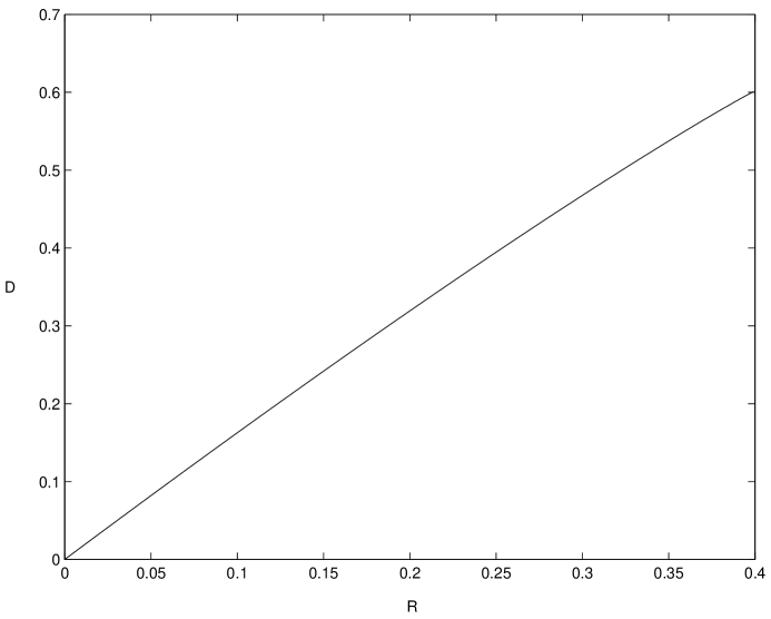
Figure 1: $D(R)$ for the two-state ensemble ${\cal E}$.

Figure 1 (cf. [19], figure 2) shows the distillable CR-rate trade-off curve $D(R)=D^{*}(R)$ for the simple two-state ensemble ${\cal E}$ given by the non-orthogonal pair $\{|0\rangle,{1\over\sqrt{2}}(|0\rangle+|1\rangle)\}$, each occurring with probability ${1\over 2}$. This curve is not much better than the linear lower bound obtained by time-sharing between $(0,0)$ and the Slepian-Wolf point $(1-H({\cal E}),H({\cal E}))$, where $H({\cal E})$ denotes the entropy of the average density matrix of the ensemble ${\cal E}$.

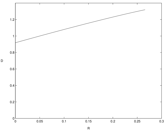
Figure 2: $D(R)$ for the three-state ensemble ${\cal E}_{3}$.

Figure 2 (cf. [19], figure 4) corresponds to the three state ensemble ${\cal E}_{3}$ consisting of the states $|\varphi_{1}\rangle=|0\rangle,|\varphi_{1}\rangle={1\over\sqrt{2}}(|0\rangle+|1\rangle)$ and $|\varphi_{3}\rangle=|2\rangle$ with equal probabilities. Without any communication it is already possible to extract $h_{2}({1\over 3})$ bits of CR, due to Bob’s ability to perfectly distinguish whether his state is in $\{|\varphi_{1}\rangle,|\varphi_{2}\rangle\}$ or $\{|\varphi_{3}\rangle\}$. The curve then follows a rescaled version of figure 1 to meet the Slepian-Wolf point $(H({1\over 3},{1\over 3},{1\over 3})-H({\cal E}_{3}),H({\cal E}_{3}))$.

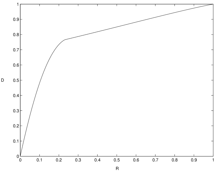
Figure 3: $D(R)$ for the parametrized BB84 ensemble with $\theta={\pi\over 8}$.

Our third example is the parametrized BB84 ensemble ${\cal E}_{\rm BB}(\theta)$, defined by the states

$$|\varphi_{1}\rangle = |0\rangle$$

$$|\varphi_{2}\rangle = \cos\theta|0\rangle+\sin\theta|1\rangle$$

$$|\varphi_{3}\rangle = |1\rangle$$

$$|\varphi_{4}\rangle = -\sin\theta|0\rangle+\cos\theta|1\rangle,$$

each chosen with probability ${1\over 4}$. The $D(R)$ curve for $\theta=\pi/8$, shown in figure 3 (cf. [19], figure 5), has a special point at which the slope is discontinuous. For $0<\theta\leq\pi/4$, ${\cal E}_{\rm BB}(\theta)$ has a natural coarse graining to the ensemble consisting of two equiprobable mixed states, ${1\over 2}(|\varphi_{1}\rangle{\langle\varphi_{1}|})+|\varphi_{2}\rangle{\langle\varphi_{2}|})$ and ${1\over 2}(|\varphi_{3}\rangle{\langle\varphi_{3}|})+|\varphi_{4}\rangle{\langle\varphi_{4}|})$. The special point is precisely the Slepian-Wolf point for this coarse-grained ensemble, treating $|\varphi_{1}\rangle$ and $|\varphi_{2}\rangle$, and $|\varphi_{3}\rangle$ and $|\varphi_{4}\rangle$ as indistinguishable.

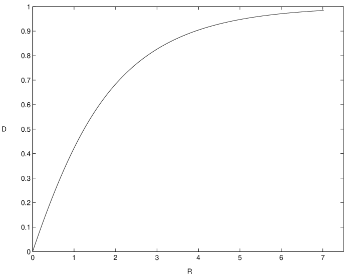
Figure 4: $D(R)$ for the uniform ensemble.

Finally, figure 4. (cf. [19], figure 5 and [15]) shows $D(R)$ for the uniform qubit ensemble, a uniform distribution of pure states over the Bloch sphere. Strictly speaking, theorem 1 should be extended to include continuous ensembles; we shall not do this here, but merely conjecture it and refer the reader to [19] for an example of such an extension. The curve approaches $D=1$ only in the $R\rightarrow\infty$ limit. It has an explicit parametrization computed from (22) and [15]:

$$R = h_{2}\left({1\over\lambda}-{1\over e^{\lambda}-1}\right)+{\lambda\over e^{\lambda}-1}-2+\log\left({\lambda e^{\lambda}\over e^{\lambda}-1}\right)$$

$$D(R) = 1-h_{2}\left({1\over\lambda}-{1\over e^{\lambda}-1}\right)\$$

for $\lambda\in(0,\infty)$, where $h_{2}(p)=-p\log p-(1-p)\log(1-p)$ is the binary Shannon entropy.

3 General quantum correlations

Consider the following double-blocking protocol for the case of $\{q\,q\}$ resources: given a word of length $nL$, Alice performs the same measurement on each of the $n$ blocks of length $L$. This leaves her with $n$ copies of the resulting $\{c\,q\}$ resource, to which we apply the $\{c\,q\}$ protocol described in the previous section. Letting $n\rightarrow\infty$ and then $L\rightarrow\infty$ yields the same results as the most general protocol described in Section 1. Let us assume $L=1$ for the moment. The measurement ${\cal M}$ on Alice’s subsystem ${\cal A}$, defined by the positive operators $(E_{x})_{x\in{\cal X}}$ with $\sum_{x}E_{x}={\mathbf{1}}$, may be thought of as a map sending a quantum system ${\cal A}{\cal B}$ in the state $\rho^{{\cal A}{\cal B}}$ to a classical-quantum system $X{\cal Q}$ in the state given by the ensemble $\{\rho_{x},p(x)\}$, where

$$p(x) = {\rm{Tr}}\,_{\!{\cal A}}\,\left(\rho^{\cal A}E_{x}\right),$$

$$\rho_{x} = {1\over p(x)}{\rm{Tr}}\,_{\!{\cal A}}\,\left((\sqrt{E_{x}}\otimes{\mathbf{1}})\rho^{{\cal A}{\cal B}}(\sqrt{E_{x}}\otimes{\mathbf{1}})\right).$$

All the relevant information is now encoded in the shared ensemble. Theorem 1 now applies, yielding an expression for the $L=1$ CR-rate curve:

$$C^{(1)}(R)=R+\max_{{\cal M}:{{\cal A}{\cal B}}\mapsto X{\cal Q}}\,\,\max_{U|X}\bigl{\{}I(U;{\cal Q})\,|\,I(U;X)-I(U;{\cal Q})\leq R\bigr{\}}.$$ (23)

Similarly we have

$$D^{(1)}(\infty)=\max_{{\cal M}:{{\cal A}{\cal B}}\mapsto X{\cal Q}}I(X;{\cal Q}),$$ (24)

which is precisely the classical correlation measure $C_{{\cal A}}(\rho^{{\cal A}{\cal B}})$ proposed in [21]. Note that w.l.o.g. we may assume the measurement to be rank-one, and $|{\cal X}|\leq d^{2}$, $d$ the dimension of the ${\cal A}$-system, because a non-extremal POVM cannot be optimal.

However, in general one must allow for “entangling” measurements performed on an arbitrary number $L$ copies of $\rho^{{\cal A}{\cal B}}$, yielding an expression for $C^{(L)}(R)$ analogous to (23):

$$C^{(L)}(R)=R+\max_{{\cal M}:{{\cal A}^{L}{\cal B}^{L}}\mapsto X{\cal Q}}\,\,{1\over L}\max_{U|X}\bigl{\{}I(U;{\cal Q})\,|\,I(U;X)-I(U;{\cal Q})\leq R\bigr{\}}.$$

Finally, taking the large $L$ limit gives

$$C(R)=\lim_{L\rightarrow\infty}C^{(L)}(R).$$

Similarly

$$D(\infty)=\lim_{L\rightarrow\infty}D^{(L)}(\infty),$$

which is the “regularized” version of $D^{(1)}(\infty)$ and the more appropriate asymmetric measure of classical correlations present in the bipartite state $\rho^{{\cal A}{\cal B}}$. It is an interesting question whether $L=1$ suffices to attain $C(R)$, or at least $D(\infty)$. In the remainder of this section we present some partial results concerning this issue.

Example 8

Let Alice and Bob switch roles: consider a state

$$\rho^{{\cal A}{\cal B}}=\sum_{x}p(x)\rho_{x}^{{\cal A}}\otimes|x\rangle{\langle x|}^{{\cal B}},$$

i.e. now Alice holds the ensemble states $\rho_{x}$ while Bob has the classical information $x$, with probability $p(x)$.

According to (24), $D^{(1)}(\infty)$ is equal to the accessible information of the state ensemble ${\cal E}=\{\rho_{x},p(x)\}$, denoted $I_{\rm acc}({\cal E})$ [22]. On the other hand, we know from [22] that $I_{\rm acc}({\cal E}\otimes{\cal E}^{\prime})=I_{\rm acc}({\cal E})+I_{\rm acc}({\cal E}^{\prime})$, for a second ensemble ${\cal E}^{\prime}$, hence

$$D(\infty)=D^{(L)}(\infty)=D^{(1)}(\infty)=I_{\rm acc}({\cal E}).$$

This single-letterization of the accessible correlation can, in fact, be generalized to arbitrary separable states. Indeed, the following holds, in some analogy to the additivity of capacity for entanglement breaking channels [33] (we include the state dependence in our notation of $D^{(1)}$ etc.):

Theorem 9

Let $\rho^{AB}$ be separable and $\sigma^{A^{\prime}B^{\prime}}$ be arbitrary. Then,

$$D^{(1)}(\rho\otimes\sigma,\infty)=D^{(1)}(\rho,\infty)+D^{(1)}(\sigma,\infty).$$

From this, by iteration, we get of course

$$D(\rho,\infty)=D^{(L)}(\rho,\infty)=D^{(1)}(\rho,\infty).$$

$\mathbf{Proof}$ $D^{(1)}(\rho\otimes\sigma,\infty)\geq D^{(1)}(\rho,\infty)+D^{(1)}(\sigma,\infty)$ is trivial for arbitrary states, for we can always use product measurements. For the opposite inequality, we write $\rho$ as a mixture of product states:

$$\rho^{{\cal A}{\cal B}}=\sum_{j}q_{j}\hat{\tau}_{j}^{{\cal A}}\otimes\tau_{j}^{{\cal B}},$$

which can be regarded as part of a classical-quantum system $J{\cal A}{\cal B}$ with EHS representation

$$\rho^{\cal J\!AB}=\sum_{j}q_{j}|j\rangle{\langle j|}^{{\cal J}}\otimes\hat{\tau}_{j}^{{\cal A}}\otimes\tau_{j}^{{\cal B}},$$

whose partial trace over ${\cal J}$ it obviously is.

Now we consider a measurement ${\cal M}=(E_{x})_{x\in{\cal X}}$ on the combined system ${\cal AA^{\prime}}$. Then, by definition, the post–measurement states on ${\cal BB^{\prime}}$ and the probabilities are given by

$$p(x)\rho_{x} = {\rm{Tr}}\,_{\!\cal AA^{\prime}}\left[\bigl{(}\rho^{\cal AB}\otimes\sigma^{\cal A^{\prime}B^{\prime}}\bigr{)}\bigl{(}E_{x}^{\cal AA^{\prime}}\otimes{\mathbf{1}}\bigr{)}\right]$$

$$= \sum_{j}q_{j}\tau_{j}^{{\cal B}}\otimes{\rm{Tr}}\,_{\!\cal AA^{\prime}}\left[\bigl{(}\hat{\tau}_{j}^{{\cal A}}\otimes\sigma^{\cal A^{\prime}B^{\prime}}\bigr{)}\bigl{(}E_{x}^{{\cal A}{\cal A}^{\prime}}\otimes{\mathbf{1}}\bigr{)}\right]$$

$$= \sum_{j}q_{j}\tau_{j}^{{\cal B}}\otimes{\rm{Tr}}\,_{\!{\cal A}^{\prime}}\left[\sigma^{\cal A^{\prime}B^{\prime}}\bigl{(}F_{x|j}\otimes{\mathbf{1}}\bigr{)}\right],$$

with the POVMs ${\cal N}_{j}=(F_{x|j})_{x\in{\cal X}}$ on ${\cal A^{\prime}}$, labeled by the different $j$:

$$F_{x|j}={\rm{Tr}}\,_{\!{\cal A}}\bigl{(}E_{x}(\hat{\tau}_{j}\otimes{\mathbf{1}})\bigr{)}.$$

Thus, applying the measurement ${\cal M}$ on ${\cal A}{\cal A}^{\prime}$ on $\rho^{\cal J\!AB}\otimes\sigma^{\cal A^{\prime}B^{\prime}}$, and storing the result in $X$ leads to the classical-quantum system $XJ{\cal B}{\cal B}^{\prime}$ defined by the EHS state

$$\omega=\sum_{x,j}|x\rangle{\langle x|}^{{\cal C}}\otimes q_{j}|j\rangle{\langle j|}^{{\cal J}}\otimes\tau_{j}^{{\cal B}}\otimes{\rm{Tr}}\,_{\!{\cal A}^{\prime}}\left[\sigma^{\cal A^{\prime}B^{\prime}}\bigl{(}F_{x|j}\otimes{\mathbf{1}}\bigr{)}\right].$$

With respect to it,

$$I(X;{\cal B}{\cal B}^{\prime}) = I(X;{\cal B})+I(X;{\cal B}^{\prime}|{\cal B})$$ (25)

$$= I(X;{\cal B})+I(X{\cal B};{\cal B}^{\prime})-I({\cal B};{\cal B}^{\prime})$$

$$= I(X;{\cal B})+I(X{\cal B};{\cal B}^{\prime})$$

$$\leq I(X;{\cal B})+I(XJ;{\cal B}^{\prime})$$

$$= I(X;{\cal B})+I(XJ;{\cal B}^{\prime})-I(J;{\cal B}^{\prime})$$

$$= I(X;{\cal B})+I(X;{\cal B}^{\prime}|J),$$

using the chain rule, the fact that ${\cal B}{\cal B}^{\prime}$ is in a product state, the data processing inequality [3], the fact that $J{\cal B}^{\prime}$ is in a product state and the chain rule once more.

In (25) notice that the first mutual information, $I(X;{\cal B})$, relates to applying the POVM ${\cal M}$ to ${\cal A}$, with an ancilla ${\cal A^{\prime}}$ in the state $\sigma^{{\cal A}^{\prime}}$ – but this can be described by a POVM ${\cal N}$ on ${\cal A}$ alone. The second, $I(X;{\cal B^{\prime}}|J)$, is a probability average over mutual informations relating to different POVMs on ${\cal A^{\prime}}$. Thus

$$I(X;{\cal BB^{\prime}})\leq D^{(1)}(\rho,\infty)+D^{(1)}(\sigma,\infty),$$

which yields the claim, as ${\cal M}$ was arbitrary.  

Example 10

For a pure entangled state $\psi=|\psi\rangle{\langle\psi|}$, we can easily see that

$$D^{(1)}(\psi,\infty)=D^{(1)}(\psi,0)=E(|\psi\rangle)=H({\rm{Tr}}\,_{\!{\cal B}}\psi).$$

Indeed, the right hand side is attained for Alice and Bob both measuring in bases corresponding to a Schmidt decomposition of $|\psi\rangle$. On the other hand, in the definition of $D^{(1)}$, eq. (24), the mutual information $I(X;{\cal Q})$ is upper bounded by $H({\cal Q})$, which is the right hand side in the above equation.

Thus, if both $\psi$ and $\varphi$ are pure entangled states,

$$D^{(1)}(\psi\otimes\varphi,\infty)=D^{(1)}(\psi,\infty)+D^{(1)}(\varphi,\infty).$$

In particular,

$$D(\psi,\infty)=D^{(L)}(\psi,\infty)=D^{(1)}(\psi,\infty).$$

More generally, we have (compare to the additivity of channel capacity if one of the channels is noiseless [31]):

Theorem 11

Let $\rho^{{\cal A}{\cal B}}=|\psi\rangle{\langle\psi|}$ be pure and $\sigma^{{\cal A}^{\prime}{\cal B}^{\prime}}$ arbitrary. Then

$$D^{(1)}(\rho\otimes\sigma,\infty)=D^{(1)}(\rho,\infty)+D^{(1)}(\sigma,\infty).$$

$\mathbf{Proof}$ As usual, only “$\leq$” has to be proved. Given any POVM ${\cal M}=(E_{x})_{x\in{\cal X}}$ on ${\cal A}{\cal A}^{\prime}$, the classical-quantum correlations $X{\cal B}{\cal B}^{\prime}$ remaining after this measurement is performed are described by

$$\omega=\sum_{x}|x\rangle{\langle x|}^{{\cal C}}\otimes{\rm{Tr}}\,_{\!\cal AA^{\prime}}\left[\bigl{(}\rho^{\cal AB}\otimes\sigma^{\cal A^{\prime}B^{\prime}}\bigr{)}\bigl{(}E_{x}^{\cal AA^{\prime}}\otimes{\mathbf{1}}\bigr{)}\right].$$

We shall assume that $|\psi\rangle$ is in Schmidt form:

$$|\psi\rangle=\sum_{j}\sqrt{\lambda_{j}}|j\rangle^{{\cal A}}|j\rangle^{{\cal B}}.$$

Measuring in the basis $|j\rangle$ on ${\cal B}$ and recording the result in orthogonal states $|j\rangle{\langle j|}$ in a register ${\cal J}$ transforms $\omega$ into the state

$$\omega^{\prime}=\sum_{x,j}\lambda_{j}|j\rangle{\langle j|}^{{\cal J}}\otimes|x\rangle{\langle x|}^{{\cal C}}\otimes{\rm{Tr}}\,_{\!\cal AA^{\prime}}\left[\bigl{(}|j\rangle{\langle j|}^{{\cal A}}\otimes\sigma^{\cal A^{\prime}B^{\prime}}\bigr{)}\bigl{(}E_{x}^{\cal AA^{\prime}}\otimes{\mathbf{1}}^{{\cal B}^{\prime}}\bigr{)}\right].$$

We claim that

$$I_{\omega}(X;{\cal BB^{\prime}})\leq I_{\omega^{\prime}}(X;{\cal B}^{\prime}|J)+H_{\omega}({\cal B}),$$ (26)

where the subscript indicates the state relative to which the respective information quantity is understood. Clearly, from this the theorem follows: on the right hand side, the entropy is the entropy of entanglement of $\rho$, and the mutual information is an average of mutual informations for measurements ${\cal M}_{j}$ on ${\cal A}^{\prime}$, defined as performing ${\cal M}$ with ancillary state $|j\rangle{\langle j|}$ on ${\cal A}$.

To prove (26), we first reformulate it such that all entropies refer to the same state. For this, observe that the measurement of $j$ can be done by adjoining the register ${\cal J}$ in a null state $|0\rangle$, applying a unitary which maps $|j\rangle^{{\cal B}}|0\rangle^{{\cal J}}$ to $|j\rangle^{{\cal B}}|j\rangle^{{\cal J}}$, and tracing out ${\cal B}$. Denote by $\Omega$ the state obtained from $\omega$ by this procedure. Obviously then, (26) is equivalent to

$$I(X;{{\cal B}{\cal J}{\cal B}^{\prime}})\leq I(X;{\cal B}^{\prime}|{\cal J})+H({\cal B}{\cal J}),$$ (27)

with respect to $\Omega$, because isometries do not alter entropies.

Now, writing out the above quantities as sums and differences of entropies, and using the fact that ${\cal B}{\cal J}-{\cal B}^{\prime}$ is in a product state, a number of terms cancel out, and (27) becomes equivalent to

$$H({\cal B}{\cal J}{\cal B}^{\prime}|X)\geq H({\cal B}^{\prime}|X{\cal J}).$$

But now rewriting the left hand side, using $H({\cal B}{\cal J}|X)\geq 0$ (because it is an average of von Neumann entropies), we estimate:

$$H({\cal B}{\cal J}{\cal B}^{\prime}|X) = H({\cal B}^{\prime}|{\cal B}{\cal J}X)+H({\cal B}{\cal J}|X)$$

$$\geq H({\cal B}^{\prime}|{\cal B}{\cal J}X)$$

$$\geq H({\cal B}^{\prime}|{\cal J}X),$$

where in the last line we have used strong subadditivity, and we are done.  

We do not know if additivity as in the above cases holds universally, but we regard our results as evidence in favor of this conjecture.

Returning to finite side-communication, it is a most interesting question whether a similar single-letterization can be performed. We do not know if an additivity-formula, similar to the one in lemma 3 for classical-quantum correlation, holds for the rate function $D^{(1)}(\rho\otimes\sigma,R)$. In fact, this seems unlikely because its definition does not even allow one to see that it is concave in $R$ (which it better had to if it be equal to the regularized quantity.). Of course this can easily be remedied by going to the concave hull $\widetilde{D}^{(1)}$ of $D^{(1)}$: note that both regularize to the same function for $L\rightarrow\infty$. However, we were still unable to prove additivity for $\widetilde{D}^{(1)}$. This would be a most desirable property, as it would allow single-letterization of the rate function just as in the case of classical-quantum correlations. As it stands, $\widetilde{D}^{(1)}(\rho,R)$ is the CR obtainable from $\rho$ in excess over $R$, if (one-way) side communication is limited to $R$ and if the initial measurement is a tensor product.

4 Discussion

We have introduced the task of distilling common randomness from a quantum state by limited classical one-way communication, placing it in the context of general resource conversion problems from classical and quantum information theory. Our exposition can be read as a systematic objective for the field of quantum information theory: to study all the conceivable inter-conversion problems between the resources enumerated in the Introduction.

Our main result is the characterization of the optimal asymptotically distillable common randomness $C$ (as a function of the communication bound $R$); in the case of initial classical-quantum correlations this characterization is a single-letter optimization.

A particularly interesting figure is the total “distillable common randomness”, which is the supremum of $C(R)-R$ as $R\rightarrow\infty$: for the classical-quantum correlations it turns out to be simply the quantum mutual information, and in general it is identical to the regularized version of the measure for classical correlation put forward by Henderson and Vedral [21].

It should be noted that this quantity is generally smaller than the quantum mutual information $I({\cal A};{\cal B})$ of the state $\rho^{{\cal A}{\cal B}}$ (which was discussed in [13]), but larger than the quantity proposed by Levitin [26]. Interestingly, while the former work simply examines a quantity defined in formal analogy to classical mutual information for its usefulness to (at least, qualitatively) describe quantum phenomena, the latter motivates the definition by recurring to operational arguments. Of course, all this shows is that there can be several operational approaches to the same intuitive concept: quantities thus defined might coincide for classical systems but differ in the quantum version.

This is what we see even within the realm of our definitions. In the classical theory [2] the total distillable CR equals the mutual information of the initial distribution, regardless of the particulars of the noiseless side communication: whether it is one-way from Alice to Bob or vice versa, or actually bidirectional, the answer is the mutual information. There are simple examples of quantum states where the total distillable common randomness depends on the communication model: the classical-quantum correlation associated with an ensemble ${\cal E}=\{\rho_{x},p(x)\}$ of states at Bob’s side (compare eq. (1)) leads to $I({\cal A};{\cal Q})=\chi({\cal E})$ if one-way communication from Alice to Bob is available. If only one-way communication from Bob to Alice is available, it is only $I_{\rm acc}({\cal E})$, the accessible information of the ensemble ${\cal E}$, which usually is strictly smaller than the Holevo information $\chi({\cal E})$ [23].

An open problem left in this work is to decide the additivity questions in section 3: is the distillable common randomness $D^{(1)}(\rho,\infty)$ additive in general? Does the rate function $D^{(1)}(\rho,R)$ obey an additivity-formula like the one in lemma 3? Finally, there is the issue of finding the “ultimate” distillable common randomness involving two-way communication.

Acknowledgments   We thank C. H. Bennett, D. P. DiVincenzo, B. M. Terhal, J. A. Smolin and R. Abbot for useful discussions. ID’s work was supported in part by the NSA under the US Army Research Office (ARO), grant numbers DAAG55-98-C-0041 and DAAD19-01-1-06. AW is supported by the U.K. Engineering and Physical Sciences Research Council.

Appendix A Appendix

We shall list definitions and properties of typical sequences and subspaces [14, 30, 37]. Consider the classical-quantum system $UX{\cal Q}$ in the state defined by the ensemble $\{p(u,x),\rho_{ux}\}$. $X$ is defined on the set ${\cal X}$ of cardinality $s_{1}$ and $U$ on the set ${\cal U}$ of cardinality $s_{2}$. Denote by $p(x)$ and $P(x|u)$ the distribution of $X$ and conditional distribution of $X|U$ respectively.

For the probability distribution $p$ on the set ${\cal X}$ define the set of typical sequences (with $\delta>0$)

$${\cal T}^{n}_{p,\delta}=\left\{x^{n}:\forall x\ |N(x|x^{n})-np(x)|\leq n{\delta}\right\},$$

where $N(x|x^{n})$ counts the number of occurrences of $x$ in the word $x^{n}=x_{1}\ldots x_{n}$ of length $n$. When the distribution $p$ is associated with some random variable $X$ we may use the notation ${\cal T}^{n}_{X,\delta}$.

For the stochastic matrix $P:{\cal U}\rightarrow{\cal X}$ and $u^{n}\in{\cal U}^{n}$ define the set of conditionally typical sequences (with $\delta>0$) by

$${\cal T}^{n}_{P,\delta}(u^{n})=\left\{x^{n}:\forall u,x\ |N((u,x)|(u^{n},x^{n}))-P(x|u)N(u|u^{n})|\leq n{\delta}\right\}.$$

When the stochastic matrix $P$ is associated with some conditional random variable $X|U$ we may use the notation ${\cal T}^{n}_{X|U,\delta}(u^{n})$.

For a density operator $\rho$ on a $d$-dimensional Hilbert space ${\cal H}$, with eigen-decomposition $\rho=\sum_{k=1}^{d}\lambda_{k}|k\rangle{\langle k|}$ define (for $\delta>0$) the typical projector as

$$\Pi^{n}_{\rho,\delta}=\sum_{k^{n}\in{{\cal T}}^{n}_{R,\delta}}|k^{n}\rangle{\langle k^{n}|}.$$

When the density operator $\rho$ is associated with some quantum system ${\cal Q}$ we may use the notation $\Pi^{n}_{{\cal Q},\delta}$.

For a collection of states ${\rho}_{u}$, $u\in{\cal U}$, and $u^{n}\in{\cal U}^{n}$ define the conditionally typical projector as

$$\Pi^{n}_{\{\rho_{u}\},\delta}(u^{n})=\bigotimes_{u}\Pi^{I_{u}}_{\rho_{u},\delta},$$

where $I_{u}=\{i:u_{i}=u\}$ and $\Pi^{I_{u}}_{\rho_{u},\delta}$ denotes the typical projector of the density operator ${\rho}_{u}$ in the positions given by the set $I_{u}$ in the tensor product of $n$ factors. When the $\{\rho_{u}\}$ are associated with some conditional classical-quantum system system ${\cal Q}|U$ we may use the notation $\Pi^{n}_{{\cal Q}|U,\delta}(u^{n})$. We shall give several known properties of these projectors, some of which are used in the main part of the paper. For any positive $\epsilon,\delta$ and $\delta^{\prime}$, some constant $c$ depending on the particular ensemble of $UX{\cal Q}$, and for sufficiently large $n\geq n_{0}(\epsilon,\delta,\delta^{\prime})$, the following hold. Concerning the quantum system ${\cal Q}$ alone:

$${\rm{Tr}}\,\Pi^{n}_{{\cal Q},\delta} \leq 2^{n(H({\cal Q})+c\delta)}$$

$${\rm{Tr}}\,\rho^{\otimes n}\Pi^{n}_{{\cal Q},\delta} \geq 1-\epsilon.$$

Concerning the classical-quantum system $X{\cal Q}$, and for $x^{n}\in{\cal T}^{n}_{X,\delta^{\prime}}$:

$${\rm{Tr}}\,\Pi^{n}_{{\cal Q}|X,\delta}(x^{n}) \leq 2^{n(H({\cal Q}|X)+c(\delta+\delta^{\prime}))}$$ (28)

$${\rm{Tr}}\,\rho_{x^{n}}\Pi^{n}_{{\cal Q}|X,\delta}(x^{n}) \geq 1-\epsilon$$

$${\rm{Tr}}\,\rho_{x^{n}}\Pi^{n}_{{\cal Q},\,\delta+|{\cal X}|\delta^{\prime}} \geq 1-\epsilon.$$ (29)

These have been proven in [36]. Finally, concerning the full classical-quantum system $UX{\cal Q}$, for $x^{n}\in{\cal T}^{n}_{X|U,\delta^{\prime}}(u^{n})$ (29) easily extends to

$${\rm{Tr}}\,\rho_{u^{n}x^{n}}\Pi^{n}_{{\cal Q}|U,\,\delta+|{\cal X}|\delta^{\prime}}\geq 1-\epsilon.$$ (30)

References

• [1] R. Ahlswede and I. Csiszár, “Common Randomness in Information Theory and Cryptography — Part I: Secret Sharing “, IEEE Trans. Inf. Theory, vol. 39, pp. 1121–1132, 1993.
• [2] R. Ahlswede and I. Csiszár, “Common Randomness in Information Theory and Cryptography — Part II: CR-capacity”, IEEE Trans. Inf. Theory, vol. 44, pp. 225–240, 1998.
• [3] R. Ahlswede and P. Löber, “Quantum data processing”, IEEE Trans. Inf. Theory, vol.47, pp. 474–478, 2000.
• [4] C. H. Bennett, H. J. Bernstein, S. Popescu and B. Schumacher, “Concentrating Partial Entanglement by Local Operations”, Phys. Rev. A, vol. 53, pp. 2046–2052, 1996.
• [5] C. H. Bennett and G. Brassard, “Quantum Cryptography: Public key distribution and coin tossing”, Proc. IEEE Int. Conf. Computers, Systems and Signal Processing (Bangalore, India), pp. 175–179, 1984.
• [6] C. H. Bennett, G. Brassard, C. Crépeau, R. Jozsa, A. Peres and W. K. Wootters, “ Teleporting an unknown quantum state via dual classical and EPR channels”, Phys. Rev. Lett., vol. 70, pp. 1895–1898, 1993.
• [7] C. H. Bennett, I. Devetak, A. Harrow, P. W. Shor and A. Winter, “The Quantum Reverse Shannon Theorem”, in preparation.
• [8] C. H. Bennett, D. P. DiVincenzo, J. A. Smolin and W. K. Wooters, “Mixed-state entanglement and quantum error correction”, Phys. Rev. A, vol. 54, pp. 3824–3851, 1996.
• [9] C. H. Bennett, P. W. Shor, J. A. Smolin and A. V. Thapliyal, “Entanglement-assisted capacity of a quantum channel and the reverse Shannon theorem”, IEEE Trans. Inf. Theory, vol. 48, pp. 2637–2655, 2002.
• [10] C. H. Bennett and S. J. Wiesner, “Communication via one- and two- particle operators on Einstein-Podolsky-Rosen states”, Phys. Rev. Lett., vol. 69, pp. 2881–2884, 1992.
• [11] T. Berger, Rate Distortion Theory, Prentice Hall, 1971.
• [12] T. M. Cover and J. A. Thomas, Elements of information theory, John Wiley & Sons, New York, 1991.
• [13] N. J. Cerf and C. Adami, “Negative entropy and information in quantum mechanics”, Phys. Rev. Lett., vol. 79, pp. 5194–5197, 1997.
• [14] I. Csiszár and J. Körner, Information Theory: Coding Theorems for Discrete Memoryless Systems, Academic Press, New York, 1981.
• [15] I. Devetak and T. Berger, “Low entanglement remote state preparation”, Phys. Rev. Lett., vol. 87, pp. 197901–197904, 2001.
• [16] I. Devetak and T. Berger, ”Quantum rate-distortion theory for memoryless sources”, IEEE Trans. Inf. Theory vol. 48, pp. 1580–1589, 2002. H. Barnum, “Quantum rate-distortion coding”, Phys. Rev. A, vol. 62, pp. 42309–42314, 2000.
• [17] I. Devetak and A. Winter, “Classical data compression with quantum side information”, quant-ph/0209029, 2002. A. Winter, Ph.D. thesis, quant-ph/9907077, 1999.
• [18] P. Hayden, M. Horodecki and B. M. Terhal, “The asymptotic entanglement cost of preparing a quantum state”, J. Phys. A: Math. Gen., vol. 34, pp. 6891–6898, 2001.
• [19] P. Hayden, R. Jozsa and A. Winter, “Trading quantum for classical resources in quantum data compression”, J. Math. Phys., vol. 43, pp. 4404–4444, 2002.
• [20] P. Hayden and A. Winter, “On the communication cost of entanglement transformations”, Phys. Rev. A, vol. 67, pp. 012326–012333, 2003. A. W. Harrow and H.-K. Lo, “A tight lower bound on the classical communication cost of entanglement dilution”, quant-ph/0204096, 2002.
• [21] L. Henderson and V. Vedral, “Classical, quantum and total correlations”, quant-ph/0105028, 2001.
• [22] A. S. Holevo, “Information theoretical aspects of quantum measurements”, Probl. Inf. Transm., vol. 9, pp. 110-118, 1973.
• [23] A. S. Holevo, ”Bounds for the quantity of information transmitted by a quantum channel”, Probl. Inf. Transm., vol. 9, pp. 177-183, 1973.
• [24] A. S. Holevo, “The Capacity of the Quantum Channel with General Signal States”, IEEE Trans. Inf. Theory, vol. 44, pp. 269-273, 1998. B. Schumacher and M. D. Westmoreland, “Sending classical information via noisy quantum channels”, Phys. Rev. A, vol. 56, pp. 131-138, 1997.
• [25]
• [26] L. B. Levitin, “Quantum Generalization of Conditional Entropy and Information”, in: $1^{\rm st}$ NASA Conf. QCQC, p. 269, 1998.
• [27] E. H. Lieb and M. B. Ruskai, “Proof of the strong subadditivity of quantum-mechanical entropy”, J. Math. Phys., vol. 14, pp. 1938–1941, 1973.
• [28] H.-K. Lo and S. Popescu, “The classical communication cost of entanglement manipulation: Is entanglement an inter-convertible resource?” Phys. Rev. Lett., vol. 83, pp. 1459–1462, 1999.
• [29] A. K. Pati, “Minimum cbits for remote preparation and measurement of a qubit”, Phys. Rev. A, vol. 63, pp. 014320–014326, 2001. H.-K. Lo, “Classical Communication Cost in Distributed Quantum Information Processing - A generalization of Quantum Communication Complexity”, quant-ph/9912009, 1999. C. H. Bennett, D. P. DiVincenzo, J. A. Smolin, P. W. Shor, B. M. Terhal and W. K. Wooters, “Remote State Preparation”, Phys. Rev. Lett., vol. 87, pp. 77902–77905, 2001. D. W. Leung and P. W. Shor, “Oblivious remote state preparation”, quant-ph/0201008, 2002. C. H. Bennett, D. W. Leung, P. Hayden, P. W. Shor and A. Winter, “Remote preparation of quantum states”, in preparation.
• [30] B. Schumacher,”Quantum coding”, Phys. Rev. A, vol. 51, pp. 2738–2747, 1995. R. Jozsa and B. Schumacher, “A new proof of the quantum noiseless coding theorem”, J. Mod. Opt, vol. 41, pp. 2343–2349, 1994.
• [31] B. Schumacher, M. D. Westmoreland, “Relative entropy in quantum information theory”, in: Quantum Computation and Quantum Information: A Millenium Volume, S. Lomonaco (ed.), American Mathematical Society Contemporary Mathematics series, 2001.
• [32] C. E. Shannon, “A mathematical theory of communication”, Bell System Tech. Journal, vol. 27, pp. 379–623, 1948.
• [33] P. W. Shor, “Additivity of the Classical Capacity of Entanglement-Breaking Quantum Channels”, J. Math. Phys., vol. 43, pp. 4334–4340, 2002.
• [34] P. W. Shor, “The quantum channel capacity and coherent information ”, lecture notes, MSRI Workshop on Quantum Computation, 2002 (Avaliable at http://www.msri.org/publications/ln/msri/2002/quantumcrypto/shor/1/). H. Barnum, E. Knill and M. A. Nielsen, “On Quantum Fidelities and Channel Capacities”, IEEE Trans. Inf. Theory, vol. 46, pp. 1317–1329, 2000. I. Devetak “The private classical information capacity and quantum information capacity of a quantum channel”, quant-ph/0304127.
• [35] B. M. Terhal, M. Horodecki, D. W. Leung and D. P. DiVincenzo, “The entanglement of purification”, J. Math. Phys., vol. 43, pp. 4286–4298, 2002.
• [36] A. Winter, ”Coding theorem and strong converse for quantum channels”, IEEE Trans. Inf. Theory, vol. 45, pp. 2481-2485, 1999.
• [37] A. Winter, “’Extrinsic’ and ’intrinsic’ data in quantum measurements: asymptotic convex decomposition of positive operator valued measures”, quant-ph/0109050, 2001.
• [38] A. Winter and R. Wilmink, unpublished.