Stability of stationary solutions of the Schrödinger-Langevin equation

Abstract.

The stability properties of a class of dissipative quantum mechanical systems are investigated. The nonlinear stability and asymptotic stability of stationary states (with zero and nonzero dissipation respectively) is investigated by Liapunov’s direct method. The results are demonstrated by numerical calculations on the example of the damped harmonic oscillator.

1. Introduction

The study of dissipative quantum mechanical systems is of widespread interest in different areas of physics [1, 2]. In several approaches the microscopic systems are embedded in an environment and the dissipation is given with a detailed description of that assumed macroscopic background. However, the structure of the environment is principally unobservable or unknown, moreover, its details are not very important but only some basic properties. Several developments of the stochastic approach to decoherence and quantum dissipation can be interpreted as a search after these important properties and get rid of the details of the background. The unacceptable negative densities in the soluble Caldeira-Leggett model [3] can be cured by additional damping terms [4] according to the requirement of positivity of the irreversible dynamics [5]. However, complete positivity alone does not give automatically physically meaningful results, there are indications that some further refinements are necessary [6, 7].

On the other hand, the approaches from the phenomenological, thermodynamic side [8, 9, 10, 11] are fighting with the right interpretation and properties of thermodynamic quantities in quantum systems.

The situation is further complicated with the fact that there is no common agreement in the nature of quantum dissipation, there is no unique quantum version of the simplest dissipative classical systems like the damped harmonic oscillator. The problem is that the lack of a uniformly accepted variational principle prevents to use normal canonical quantization [12]. Hence quantization can be accomplished in several different ways and the quantizations based on different variational principles are not equivalent at all, moreover show peculiar physical properties. The best example and a kind of parade ground of the different methods is the mentioned quantum harmonic oscillator with the simplest possible damping [13, 14].

In this paper we approach dissipation in quantum mechanics from a different point of view and, instead of the von Neumann equation, we investigate the properties of some simple generalizations of the Schrödinger-Langevin equation, where the damping force is negatively proportional to the velocity

(1) $$i\hbar\frac{\partial\psi}{\partial t}=-\frac{\hbar^{2}}{2m}\Delta\psi+U\psi-\frac{i\hbar k}{2}\hskip 1.29167pt\psi\ln\frac{\psi}{\psi^{*}}.$$

The above equation is a quantized form of Newton equation of a classical mass-point with mass $m$, moving in a potential $U$ and with damping term proportional to velocity

(2) $$m\ddot{{\bf x}}=m\dot{{\bf v}}=-\nabla U-k{\bf v}.$$

One can give several derivations of Schrödinger-Langevin equation based on different assumptions [15, 16, 17, 18, 12, 19, 20] and the equation has several appealing properties. It can be derived by canonical quantization, the dissipation term has a clear physical meaning, the equation preserves the uncertainty relations, and all the stationary states of a quantized Hamiltonian system are necessarily stationary states of the corresponding dissipative quantum system. The later property can be true in more general systems, too [21]. At the first glance this last fact seems to be in contradiction with the apparent instability of excited states [22] and incited some criticism [23] therefore it requires a more detailed investigation that can be expected partially from stability investigations. The relationship between the Schrödinger-Langevin equation and the master equation approaches is important also from fundamental theoretical point of view, as it was indicated for example in [24].

There are some known exact solutions of equation (1) for the cases of free motion, motion in a uniform field, and for a harmonic oscillator in one dimension [25, 26]. These exact solutions have the remarkable property that the stationary states of the system are asymptotically stable.

We will show that the above properties are valid not only for these known exact solutions of the damped harmonic oscillator but in general for any kind of initial conditions, moreover not only for the oscillator, but in case of (almost) arbitrary potentials. The stability investigation is based on the hydrodynamic model of quantum mechanics, which recently gained a renewed interest because of the development of powerful numerical codes of computational fluid dynamics [27, 28, 29, 30, 31], and of its relationship to some quantum field theories as non-Abelian fluid dynamics [32], in perturbational cosmological calculations curing some instabilities of the Euler equation [33], etc. In the last section the above properties will be demonstrated numerically on the traditional parade ground of dissipative quantum mechanics, on the example of the damped harmonic oscillator.

2. Stability properties of the damped Schrödinger equation

Let us consider a classical mass-point with mass $m$, moving in a potential $U$, governed by the following Newton equation:

(3) $$m\frac{{\rm d}^{2}{\bf x}}{{\rm d}t^{2}}=m\frac{{\rm d}{\bf v}}{{\rm d}t}=-\nabla U+{{\bf F}_{\rm d}},$$

where $U$ is the potential of the conservative part, ${{\bf F}_{\rm c}}=-\nabla U$, of the total force.

It is well-known that the equation of motion of the corresponding quantized system can be given when ${{\bf F}_{\rm d}}={\bf 0}$ and is the Schrödinger equation, (1) with $k=0$. The Schrödinger equation can be transformed into various thought provoking classical forms via the Madelung transformation

$$\psi=Re^{iS},$$

and by introducing the so-called hydrodynamic variables, defining the probability density $\rho$ and a velocity field ${\bf v}$ as

(4) $$\rho :=R^{2}=\psi^{*}\psi,$$

(5) $${\bf v} :=\frac{\hbar}{m}\hskip 1.29167pt\nabla S=-\frac{i\hbar}{2m}\hskip 1.29167pt\nabla\ln\frac{\psi}{\psi^{*}}.$$

Here the star denotes the complex conjugate. With these variables the real and imaginary parts of the Schrödinger equation give

(6) $$\frac{\partial\rho}{\partial t} +\nabla\hskip-0.6458pt\cdot\hskip-0.6458pt(\rho{\bf v})=0,$$

(7) $$m\frac{\partial{\bf v}}{\partial t} =-\nabla\left(m\frac{v^{2}}{2}+U_{q}+U\right),$$

with the condition that the vorticity of the “fluid” is zero:

(8) $$\omega=\nabla\times{\bf v}={\bf 0}.$$

Here

$$U_{q}=-\frac{\hbar^{2}}{2m}\frac{\Delta R}{R}=-\frac{\hbar^{2}}{4m\rho}\left(\Delta\rho-\frac{(\nabla\rho)^{2}}{2\rho}\right)$$

is sometimes called the quantum potential, and the equations (6)-(7) are governing equations of the fields $(\rho,{\bf v})$. In particular, (6) is the balance of “mass” or probability density. The second equation (7) is the Newtonian equation for a point mass moving in superposed normal and quantum potentials. The governing equations are more apparent if we transform them into a ‘comoving’ form:

(9) $$\dot{\rho}+\rho\nabla\hskip-0.6458pt\cdot\hskip-0.6458pt{\bf v} =0,$$

(10) $$m\dot{\bf v} =-\nabla\left(U_{q}+U\right).$$

Here the dot derivative denotes the substantial time derivative, $\partial_{t}+{\bf v}\hskip-0.6458pt\cdot\hskip-0.6458pt\nabla$. It is easy to see that the above equations preserve the probability and vorticity. In the hydrodynamic formalism it is apparent that any other kind of dissipative forces that would destroy the condition of zero vorticity would destroy the connection to the single Schrödinger equation and initiate coupling to the electromagnetic field or/and the development from pure into mixed states. It is straightforward to transform the above system into a true hydrodynamic form, because the quantum potential can be pressurised that is, the corresponding force density can be written as a divergence of a quantum pressure tensor $P_{q}$:

$$\rho\nabla U_{q}=\nabla\hskip-0.6458pt\cdot\hskip-0.6458ptP_{q},$$

where the quantum pressure is not determined uniquely from this condition. It can be chosen as

$$P_{q_{1}}=-\frac{\hbar^{2}}{4m\rho}\left(\Delta\rho\hskip 1.29167ptI-\frac{\nabla\rho\circ\nabla\rho}{\rho}\right),$$

or as

$$P_{q_{2}}=-\frac{\hbar^{2}}{4m\rho}\left[(\nabla\circ\nabla)\rho-\frac{\nabla\rho\circ\nabla\rho}{\rho}\right]=\frac{\hbar^{2}}{4m}(\nabla\circ\nabla)\ln\rho,$$

or in some other form that differs only in a rotation of a vector field. Here $\circ$ is the traditional notation of tensorial product in hydrodynamics, and $I$ is the second order unit tensor. Let us remark that thermodynamic considerations result in a unique quantum pressure [34]. Therefore, the second equation of the above system, (10), can be written in a true Cauchy form momentum balance as well, introducing the mass density $\tilde{\rho}=m\rho$,

(11) $$\frac{\partial\tilde{\rho}}{\partial t}+\nabla\hskip-0.6458pt\cdot\hskip-0.6458pt(\tilde{\rho}{\bf v}) =0,$$

(12) $$\frac{(\partial\tilde{\rho}{\bf v})}{\partial t}+\nabla\left(\tilde{\rho}{\bf v}\circ{\bf v}+P_{q}\right) =-\tilde{\rho}\nabla U.$$

All these kinds of transformations of the Schrödinger equation are well- known in the literature with different interpretations. The Newtonian form was investigated and popularized e.g. by Bohm and Holland [35, 36]. The hydrodynamic form was first recognized by Madelung [37]) and extensively investigated by several authors, e.g. [38, 39, 40]. Moreover there is also a microscopic-stochastic background [41, 42, 43, 44], giving a reasonable explanation of the continuum equations. Independently of the interpretation, one can exploit the advantages of the hydrodynamic formulation to solve the equations or investigating its properties.

First of all let us remark that the quantum mechanical equation (10) can be supplemented by forces that are not conservative in classical mechanics but still admit a hydrodynamic formulation:

(13) $$m\dot{\bf v}=-\nabla\left(U_{q}+U\right)+{{\bf F}_{\rm d}}({\bf v}).$$

The corresponding balance of momentum is

(14) $$\frac{(\partial\tilde{\rho}{\bf v})}{\partial t}+\nabla\left(\tilde{\rho}{\bf v}\circ{\bf v}+P_{q}\right)=\tilde{\rho}\left(-\nabla U+{{\bf F}_{\rm d}}\right).$$

It is easy to check that all force fields of the form ${{\bf F}_{\rm d}}=-k(S){\bf v}$ are rotation free, therefore do not violate the vorticity conservation and the corresponding quantized form can be calculated by canonical quantization with the help of the velocity potential $S$ [16]. The hydrodynamic transformation gives the quantized form of the damping force expressed with the wave function as ${{\bf F}_{\rm d}}=-\frac{i\hbar k(S)}{2}\nabla\ln\frac{\psi}{\psi^{*}}$. Moreover, the Schrödinger equation is transformed into the Schrödinger-Langevin form (1). Let us mention here that the nonlinearity of equation (1) means only a practical, not a fundamental problem [20].

The real stationary solutions of the above system are those where the substantial time derivatives are zero. Thus we can eliminate the virtual effect of the motion of the continuum, and the stationary solution will not depend on any kind of external observers, stationarity becomes a frame independent property. Then, the nontrivial ($\rho\neq 0$) stationary solutions ($\rho_{s},{\bf v}_{s}$) coincide with the stationary solutions of the Schrödinger equation without damping, and in the hydrodynamic language are characterized by the conditions,

(15) $${\bf v}_{s} =0,$$

(16) $$U_{q}(\rho_{s})+U =E_{s}={\it const.}$$

For the sake of simplicity, in what follows we choose units in which $\hbar=1$ and $m=1$ and which make all quantities dimensionless.

In the following we investigate the stability of the stationary solutions (15)-(16) of the equations (11) and (14).

Let us assume that the functions $(\rho,{\bf v})$ are two times continuously differentiable and the density $\rho_{s}$ exponentially tend to zero as $|{\bf x}|$ goes to infinity

(17) $$\lim_{|{\bf x}|\rightarrow\infty}\rho_{s}(\bf x)e^{|{\bf x}|}=0.$$

Furthermore the dissipative force obeys the following inequality for all possible solutions of the above equations (11) and (14)

(18) $$\int\rho{\bf v}\hskip-0.6458pt\cdot\hskip-0.6458pt{{\bf F}_{\rm d}}\hskip 1.29167pt{\rm d}V\leq 0.$$

Here equality is valid only if $\rho{\bf v}_{s}=0$.

With these conditions we show that

(19) $$L(\rho,{\bf v})=\int\rho\left[\frac{v^{2}}{2}+\frac{1}{2}\left(\frac{\nabla\rho}{2\rho}\right)^{2}+U-E_{s}\right]{\rm d}V$$

is a Liapunov functional for the stationary solution in question.

First we show that, (19) is decreasing along the solutions of the differential equation. Indeed, the first derivative (variation) of $L$ for $\begin{pmatrix}\delta\hskip-0.6458pt\rho&\delta{\bf v}\end{pmatrix}$ is

$$\delta L=\int\left[\rho{\bf v}\delta{\bf v}+\left(\frac{v^{2}}{2}+U+U_{q}-E_{s}\right)\delta\hskip-0.6458pt\rho\right]{\rm d}V+\oint\frac{\nabla\ln\rho}{4}\hskip 1.29167pt\delta\hskip-0.6458pt\rho\hskip-0.6458pt\cdot\hskip-0.6458pt{\rm d}{\bf A},$$

where the surface for the second integral is a sphere with the radius increasing to infinity. That term zero at the corresponding equilibrium (stationary) solution under the asymptotic condition (17). Therefore the derivative according to the differential equation is

(20) $$\frac{{\rm d}L}{{\rm d}t}=-\oint\left[\rho{\bf v}\left(\frac{v^{2}}{2}+U_{q}+U-E_{s}\right)+\frac{\nabla\hskip-0.6458pt\ln\hskip-0.6458pt\rho\hskip 2.58334pt\nabla\hskip-0.6458pt\cdot\hskip-0.6458pt(\rho{\bf v})}{4}\right]\hskip-0.6458pt\cdot\hskip-0.6458pt{\rm d}{\bf A}+\int\rho{\bf v}\hskip-0.6458pt\cdot\hskip-0.6458pt{{\bf F}_{\rm d}}\hskip 1.29167pt{\rm d}V\leq 0,$$

because the first surface integral vanishes according to the asymptotic conditions, and the second integral is negative due to (18).

Next, the definiteness of the second derivative of (19) is investigated. Evaluating the second variation between $\begin{pmatrix}\delta\hskip-0.6458pt\rho&\delta{\bf v}\end{pmatrix}$ and $\begin{pmatrix}\delta^{\prime}\hskip-0.6458pt\rho&\delta^{\prime}{\bf v}\end{pmatrix}$ that yields

(21) $$\int\begin{pmatrix}\delta{\bf v}&\delta\hskip-0.6458pt\rho&\nabla\delta\hskip-0.6458pt\rho\end{pmatrix}\begin{pmatrix}\rho&{\bf v}&{\bf 0}\\ {\bf v}&\frac{(\nabla\rho)^{2}}{4\rho^{3}}&-\frac{\nabla\rho}{4\rho^{2}}\\ {\bf 0}&-\frac{\nabla\rho}{4\rho^{2}}&\frac{1}{4\rho}\end{pmatrix}\begin{pmatrix}\delta^{\prime}{\bf v}&\delta^{\prime}\hskip-0.6458pt\rho&\nabla\delta^{\prime}\hskip-0.6458pt\rho\end{pmatrix}{\rm d}V.$$

We can see that the minors of the above matrix under the integration are

(22) $$\Delta_{1}=\rho,\qquad\Delta_{2}=\left(\frac{\nabla\rho}{2\rho}\right)^{2}-{\bf v}^{2},\qquad\Delta_{3}=-\frac{{\bf v}^{2}}{4\rho}.$$

The matrix in (21) is positive semidefinite in case of stationary solutions, therefore the linearized system is marginally stable.

Remarks:

• The continuity and asymptotic conditions are valid for stationary solutions in case of several classical potentials (harmonic, Coulomb, etc..). Moreover, one can find different (weaker) asymptotic conditions to ensure the differentiability of L.

• The physical meaning of the Liapunov function (19) is that it is essentially the expectation value of the energy difference of the given and the stationary states. The decreasing property of $L$ is simply the decreasing of energy in our dissipative system. The Liapunov function can be expressed with the wave function as

  (23) $$\hat{L}(\psi)=-\int\left(\frac{\psi^{*}}{8\psi}(\nabla\psi)^{2}+\frac{\psi}{8\psi^{*}}(\nabla\psi^{*})^{2}+(U-E_{e})\psi\psi^{*}\right){\rm d}V$$

• According to the structure of the second derivative of $L$, given in (21), the function space of $(\rho,{\bf v})$ functions looks like a Soboljev space with our asymptotic conditions and norm

  $$\|(\rho,{\bf v})\|_{\rm S}=\left\{\int\left[\rho^{2}+{\bf v}^{2}+(\nabla\rho)^{2}\right]{\rm d}V\right\}^{1/2}$$

• If ${{\bf F}_{\rm d}}\equiv{\bf 0}$ then the equilibrium solution is stable with the above conditions. We can see that the dissipative, damping force makes the stationary solutions attractive, therefore we can expect asymptotic stability (the conditions can be rather involved see e.g. [45]). In ordinary quantum mechanics without damping forces the stationary solutions can be only stable. Furthermore, the above condition can serve as a definition of damping (dissipative) forces, i.e. we can say that a force is damping (dissipative) if $\rho{\bf v}\hskip-0.6458pt\cdot\hskip-0.6458pt{{\bf F}_{\rm d}}\leq 0$ and $\int\rho{\bf v}\hskip-0.6458pt\cdot\hskip-0.6458pt{{\bf F}_{\rm d}}\hskip 1.29167pt{\rm d}V<0$ for any configuration $\rho,{\bf v}$.

• The marginal stability indicates a rich structure of possible instabilities and therefore the need of further stability investigations. On the other hand a rich stability structure is expected considering the infinite number of stationary states. Moreover, in more than one dimension and if the domain of the functions $(\rho,{\bf v})$ is not the whole space (e.g. in case of a Coulomb potential), the perturbations destroying the rotation free streams requires to consider Casimir functions for the stability investigations [45, 46].

• The given conditions are capable to estimate the basin of attraction of the different quantum states. The physical role of dissipation is to relax the process to the lowest energy element within a basin of attraction. Moreover, the above local (!) statement regarding the formal stability of stationary states does not exclude the possibility that for a given initial condition the whole set of stationary solution is the attractor of the quantum dynamics. On the other hand transition from one basin to another possibly can be induced by some additional interaction introduced in the system.

3. Stability properties of the harmonic oscillator

As a demonstration of the previous stability properties we investigate the one dimensional dissipative harmonic oscillator, with constant damping coefficient. In this case the hydrodynamic equations are simplified into the following form

(24) $$\frac{\partial\rho}{\partial t} =-\frac{\partial(\rho v)}{\partial x},$$

(25) $$m\frac{\partial v}{\partial t} =-\frac{\partial}{\partial x}\left[m\frac{v^{2}}{2}-\frac{\hbar^{2}}{4m\rho}\left(\frac{\partial^{2}\rho}{\partial x^{2}}-\frac{1}{2\rho}\left(\frac{\partial\rho}{\partial x}\right)^{2}\right)-D\frac{x^{2}}{2}\right]-kv.$$

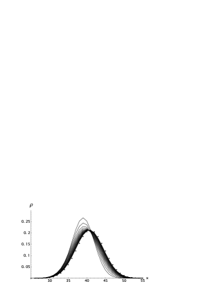
Let the initial condition be a standing wave packet ($v_{\mathrm{init}}=0$), having the shape $\rho_{\mathrm{init}}=\rho_{(0,0.05)}$, and with its maximum shifted from the center of the oscillator potential to the left by two units. We will investigate the time development of this initial distribution in a potential with elasticity coefficient $D=0.02$ and different damping coefficients. In the numerical calculations the equations have been solved with a modified leapfrog method, adapted to the presence of the nonlinear hydrodynamic term and for dissipative forces. The asymptotic conditions at the infinity were considered by extrapolating the internal velocity values at the boundaries.

On the first two figures one can see the time development of the probability distribution and the current, respectively. In this calculations the damping was large, with a coefficient $k=1$. On figure 1 the center of the oscillator is at point 41 and the solutions starting from $\rho_{(0,0.05)}$ are given in every 5 time units from 0 to 100. One can observe that the distribution tends toward the stationary solution, denoted by dots. At the same time, the probability current goes to zero as one can see on figure 2. It is interesting to observe that, in the beginning, there is a space interval where the velocity is negative and later the direction of the motion become everywhere positive.

Figure 1. $k=1$, large damping. Probability distribution of the position, $t=0,...,100$, in every 5 time units.

Figure 2. $k=1$, large damping. Probability current of the position, $t=0,...,100$, in every 5 time units.

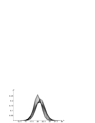
At the calculations leading to the next two figures the damping was smaller, with a coefficient $k=0.1$. On figure 3 the center of the oscillator is at point 21 and the solutions are given in every 1 time units from 0 to 20. One can observe that the trend to equilibrium is different from that of the previous case. A new period of a damped oscillation starts, as one can conclude from figure 4 of the probability current.

Figure 3. $k=0.1$, small damping. Probability distribution of the position, $t=0,...,20$, in every 1 time units.

Figure 4. $k=0.1$, small damping. Probability current of the position, $t=0,...,26$, in every 1.3 time units.

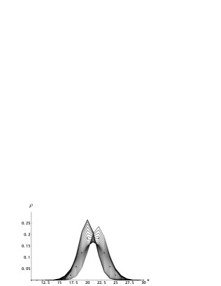
At figures 5-6 there are the undamped solutions with $k=0$. The center of the oscillator is at point 21 and the solutions starting from $\rho_{(0,0.05)}$ are given in every 0.95 time units from 0 to 19.

Figure 5. $k=0$, zero damping. Probability distribution of the position, $t=0,...,19$, in every 0.95 time units.

Figure 6. $k=0$, zero damping. Probability current of the position, $t=0,...,19$, in every 0.95 time units.

On figure 7 one can see the $L^{2}$ distance from the stationary solution in the three cases as a function of time. Remarkably, the starting oscillations are clearly nonlinear. The new, starting periods indicate clearly that the $L^{2}$ norm is not the suitable one for stability considerations. The expected asymptotic stability requires a monotonous tending to the stationary solution.

Figure 7. $L^{2}$ distance from the equilibrium. $k=0,0.1,1$ at the dotted, continuous and dashed lines respectively.

4. Conclusions

The stability properties of the stationary solutions of the Schrödinger equation were investigated. It has been shown that the stability of stationary states can be treated by Liapunov’s direct method, where the expectation value of the energy is a good starting point for stability investigations. However, the semidefiniteness of the second derivative at the stationary states and the infinite number of stationary solutions of the equation indicates a rich stability structure. These properties are more apparent in the chosen hydrodynamic model of quantum mechanics, enabling the use of the methods and a direct comparison of the well understood hydrodynamic stability problems. Moreover, the hydrodynamic analogy shows that in one space dimension we do not need Casimirs therefore the energy is also sufficient for exact and physically relevant results.

We have shown that in the nondissipative case, for the Shrödinger equation one can expect only stability. Moreover, the above properties were demonstrated for the damped harmonic oscillator. This property indicates that an arbitrarily perturbed nondissipative quantum system cannot move from a given stationary state to an other one, it will oscillate around the perturbed state.

Finally we would like to emphasize again that the stability results are independent on any interpretation and could be formulated with the help of wave functions or stochastic processes, too. However, in case of dissipation the hydrodynamic formulation has the advantage of a clear nonequilibrium thermodynamic background with well established stability results and clean concepts of dissipation. This kind of distinction of dissipation types can be crucial if one would like to compare and extend the above calculations to successful and experimentally tested frictional models as e.g. the one of Gross and Kalinowski for heavy ion collisions [47, 48].

5. Acknowledgements

This research was supported by OTKA T034715 and T034603. The authors thank T. Matolcsi, J. Verhás, S. Katz, F. Bazsó and K. Oláh for the enlightening and interesting discussions on the foundations and paradoxes of quantum mechanics. The calculations have been performed by the software Mathematica. Thank for our referee for his/her valuable remarks.

References

- [1] U. Weiss. Quantum dissipative systems. World Scientific, Singapore, 1993.
- [2] M. B. Mensky. Continuous quantum measuremnets and path integrals. Institute of Physica Publishing, Bristol and Philadelphia, 1993.
- [3] A. O. Caldeira and A. J. Leggett. Path integral approach to quantum Brownian motion. Physica A, 121:587–616, 1983.
- [4] L. Diósi. Caldeira-Leggett master equation at medium temperatures. Physica A, 199:517–526, 1993.
- [5] G. Lindblad. Completely positive maps and entropy inequalities. Communications in Mathematical Physics, 40(2):147–151, 1975.
- [6] B. Vacchini. Completely positive quantum dissipation. Physical Review Letters, 84(7):1374–1377, 2000.
- [7] P. Földi, A. Czirják, and M. G. Benedict. Rapid and slow decoherence in conjunction with dissipation on a system of two-level atoms. Physical Review A, 63:033807, 2001.
- [8] G. P. Beretta. A theorem on Lyapunov stability for dynamical systems and a conjecture on a property of entropy. Journal of Mathematical Physics, 27(1):305–308, 1985.
- [9] W. Muschik and M. Kaufmann. Quantum-thermodynamical description on discrete non-equilibrium systems. Journal of Non-Equilibrium Thermodynamics, 19(1):76–94, 1994.
- [10] A. Kato, M. Kaufmann, W. Muschik, and D. Schirrmeister. Different dynamics and entropy rates in quantum-thermodynamics. Journal of Non-Equilibrium Thermodynamics, 25(1):63–86, 2000.
- [11] M. Kaufmann. Quantum Thermodynamics of Discrete Systems Endowed with Time Dependent work Variables and Based on a Dissipative v. Neumann Equation. PhD thesis, Technical University of Berlin, Berlin, September 1996. Wissenschaft und Technik Verlag, Berlin.
- [12] A. O. Bolivar. Quantization of non-Hamiltonian physical systems. Physical Review A, 58(6):4330–4335, 1998.
- [13] J. Cislo and J. Lopuszański. To what extent do the classical equations of motion determine the quantization scheme? Journal of Mathematical Physics, 42(11):5163–5176, 2001.
- [14] C.-I. Um, K.-H. Yeon, and T. F. George. The quantum damped harmonic oscillator. Physics Reports, 362:63–192, 2002.
- [15] M. D. Kostin. On the Schrödinger-Langevin equation. The Journal of Chemical Physics, 57(9):3589–3590, 1972.
- [16] K. K. Kan and J. J. Griffin. Quantized friction and the correspondence principle: single particle with friction. Physics Letters, 50B(2):241–243, 1974.
- [17] K. Yasue. Stochastic quantization: A review. International Journal of Theoretical Physics, 18(12):861–913, 1979.
- [18] H. Dekker. Classical and quantum mechanics of the damped harmonic oscillator. Physics Reports, 80(1):1–112, 1981.
- [19] R. J. Wysocki. Quantum equations of motion for a dissipative system. Physical Review A, 61(022104), 2000.
- [20] T. Fülöp and S. D. Katz. A frame and gauge free formulation of quantum mechanics. quant-ph/9806067, 1998.
- [21] V. E. Tarasov. Stationary states of open quantum systems. Physical Review E, 66:056116, 2002.
- [22] S. Gao. Dissipative quantum dynamics with a Lindblad functional. Physical Review Letters, 79(17):3101–3105, 1997.
- [23] D. M. Greenberger. A critique of the major approaches to damping in quantum theory. Journal of Mathematical Physics, 20(5):762–770, 1979.
- [24] A. O. Caldeira and A. J. Leggett. Influence of damping on quantum interference: An exactly soluble model. Physical Review A, 31:1059–1063, 1985.
- [25] R. W. Hasse. On the quantum mechanical treatment of dissipative systems. Journal of Mathematical Physics, 16(10):2005–2011, 1975.
- [26] B.-S. K. Skagerstam. Stochastic mechanics and dissipative forces. Journal of Mathematical Physics, 18:308–311, 1975.
- [27] C. L. Lopreore and R. E. Wyatt. Quantum wave packet dynamics with trajectories. Physical Review Letters, 82(26):5190–5193, 1999.
- [28] X.-G. Hu, T.-S. Ho, H. Rabitz, and A. Askar. Solution of quantum fluid dynamical equation with radial basis function interpolation. Physical Review E, 61(5):5967–5976, 2000.
- [29] E. R. Bittner. Quantum tunelling dynamics using hydrodynamic trajectories. Journal of Chemical Physics, 112(22):9703–9710, 2000.
- [30] J. B. Maddox and E. R. Bittner. Quantum relaxation dynamics using bohmian trajectories. Journal of Chemical Physics, 115(14):6309–6316, 2001.
- [31] A. Donoso and C. C. Martens. Quantum tunelling using entangled trajectories. Physical Review Letters, 87(223202), 2001.
- [32] B. Bistrovic, R. Jackiw adn H. Li, V. P. Nair, and S.-Y. Pi. Non-Abelian fluid dynamics in Lagrangian formulation. (hep-th/0210143), 2002.
- [33] I. Szapudi and N. Kaiser. Cosmological perturbation theory using the Schrödinger equation. astro-ph/0211065, 2002.
- [34] P. Ván and T. Fülöp. Weakly nonlocal fluid mechanics - the Schrödinger equation. (quant-ph/0304062), 2003.
- [35] D. Bohm. Quantum Theory. Prentice-Hall, New York, 1951.
- [36] P. R. Holland. The Quantum Theory of Motion. Cambridge University Press, Cambridge, 1993.
- [37] E. Madelung. Quantentheorie in hydrodynamischer Form. Zeitschrift für Physik, 40:322–326, 1926. in German.
- [38] L. Jánossy and M. Ziegler. The hydrodynamical model of wave mechanics I., (the motion of a single particle in a potential field). Acta Physica Hungarica, 16(1):37–47, 1963.
- [39] L. Jánossy and M. Ziegler-Náray. The hydrodynamical model of wave mechanics II., (the motion of a single particle in an external electromagnetic field). Acta Physica Hungarica, 16(4):345–353, 1964.
- [40] T. C. Wallstrom. Inequivalence between the Schrödinger equation and the Madelung hydrodynamic equations. Physical Review A, 49(3):1613–1617, 1994.
- [41] I. Fényes. Eine wahrscheinlichkeitstheoretischi Begründung und Interpretation der Quantenmechanik. Zeitschrift für Physik, 132:81–106, 1952. in German.
- [42] E. Nelson. Derivation of the Schrödinger equation from Newtonian mechanics. Physical Review, 150(4):1079–1085, 1966.
- [43] L. de la Pe a and A. M. Cetto. The Quantum Dice (An Introduction to Stochastic Electrodynamics). Kluwer Academic Publishers, Dordrecht-Boston-London, 1996.
- [44] Fritcshe L. and M. Haugk. A new look at the derivation of the Schrödinger equation from Newtonian mechanics. Annalen der Physik (Leipzig), 12:371–403, 2003.
- [45] D. D. Holm, J. E. Marsden, T. Ratiu, and A. Weinstein. Nonlinear stability of fluid and plasma equilibria. Physics Reports, 123(1):1–116, 1985.
- [46] V. I. Arnold. On an a priori estimate in the theory of hydrodynamic stability. English transl: Am. Math. Soc. Transl., 19:267–269, 1969.
- [47] D. H. E. Gross. Theory of nuclear friction. Nuclear Physics A, A240:472–484, 1975.
- [48] D. H. E. Gross and H. Kalinowski. Friction model of heavy ion collisions. Physics Reports, 45(3):176–210, 1978.