Testing Bell’s inequality and measuring the entanglement using superconducting nanocircuits
Abstract
An experimental scheme is proposed to test Bell’s inequality by using superconducting nanocircuits. In this scheme, quantum entanglement of a pair of charge qubits separated by a sufficiently long distance may be created by cavity quantum electrodynamic techniques; the population of qubits is experimentally measurable by dc currents through the probe junctions, and one measured outcome may be recorded for every experiment. Therefore, both locality and detection efficiency loopholes should be closed in the same experiment. We also propose a useful method to measure the amount of entanglement based on the concurrence between Josephson qubits. The measurable variables for Bell’s inequality as well as the entanglement are expressed in terms of a useful phase-space Q function.
pacs:
03.65.Ud, 85.25.Cp, 85.35.-pI Introduction
Recently, with the development of experimental techniques and the growing interest in quantum information, more and more attention has been devoted to experimentally testing the violation of Bell’s inequalityBell , as well as measuring the amount of entanglement of entangled particles. Entanglement of particles, an idea introduced in physics by the famous Einstein-Podolsky-Rosen (EPR) gedanken experiment EPR , is one of the most strikingly nonclassical features of quantum theory. In quantum mechanics, particles are called entangled if their states can not be factored into single-particle states. This inseparability leads to a stronger correlation between entangled quantum systems than classical ones. Since Bell’s pioneering workBell that EPR’s implication to explain the correlations using hidden parameters would contradict the predictions of quantum physics, a number of experimental tests have been performedAspect ; Shih ; Ou ; Tittel ; Weihs ; Rowe . Many of these experiments Aspect ; Shih ; Ou ; Tittel ; Weihs have been done by using photons to prepare EPR pairs. Very recently, trapped atoms were also used in the experimentRowe for testing Bell’s inequality to raise the efficiency when reading out the state. The violation of Bell’s inequality may be considered as a manifestation of the irreconcilability of quantum mechanics and “local realism”, and all recent experiments have agreed with the predictions of quantum mechanics.
Nevertheless, two important experimental loopholes mean that the evidence reported in the previous experiments was inclusiveloophole ; Grangier . The first of these loopholes is the so-called locality loophole: whenever measurements are performed on two spatially separated particles, any possibility of signals propagating with a speed equal to or less than the velocity of light between the two parts of the apparatus must be excluded. This loophole was closed in the experiments reported in Refs.Tittel ; Weihs . The second one is referred to as the detection-efficiency loophole, which argues that in most optical experiments, only a very small fraction of the particles generated are actually detected. So it is possible that for each measurement, the statistical sample provided by the detector is biased. Since improving the detection efficiency in experiments with pairs of entangled photons is found to be more difficult than expected, closing this loophole experimentally is achieved by using two massive entangled trapped ionsRowe , where the states are easier to be detected than those of photons. But the experimentRowe does not close the locality loophole. To close both loopholes in the same experiment remains to be a big challenge at presentGrangier .
In this paper, we propose a scheme to test Bell’s inequality in the Clauser, Horne, Shimony and Holt (CHSH)Clauser type and to measure the entanglement in superconducting nanocircuits. At first glance, the possibility of testing Bell’s inequality in this system may seem to be a trivial generalization of the corresponding tests by using photonsAspect ; Shih ; Ou ; Tittel ; Weihs or trapped ionsRowe . However, we show that the experiment proposed here has its own advantages. First, it is possible that both loopholes mentioned above may be closed in the same experiment. Thus, the loophole-free experiment proposed here may lead to a full logically consistent rejection of any local realistic hypothesisGrangier . Recently, very promising development was reported for Josephson-junction qubits under controlJosephson ; Nakamura ; Pashkin ; Zhu_prl2002 . The charge state in a superconducting box may be considered as a qubit system. We first address how to prepare a pair of entangled charge qubits in a sufficiently long distanceZhu , which fully enforces the requirement for strict relativistic separation between measurements. Contrary to the experiments using photons, where many photon pairs are missed, the charge states in the superconducting boxes may be detected in every measurement, thus the data in Bell’s experiments are obtained using the outcome of every experiment, thereby no fair-sampling hypothesis is required. Consequently, both the locality loophole and the efficiency loophole should be closed in the same experiment proposed here. Second, quantum mechanics violates Bell’s inequality for a state of -qubit system by an amount that grows exponentially with Mermin . The nature of being solid-state based makes Josephson junction system large-scalable, that is, the Greenberger-Horne-Zeilinger (GHZ) state [the maximally entangled states of particles ]GHZ may be achieved, in principle, in superconducting nanocircuits. However, due to experimental techniques, it is very hard to obtain many-particle entangled states in realistic experiments with photons or trapped atoms. Last, but not the least, the Josephson junction system proposed here is a mesoscopic system. Comparing with the systems consisting of a small number of microscopic particles, such as photons or trapped ions, where quantum entanglement is generally believed to exist, the superconducting box considered here involves a huge number of Cooper pairs. To test the nonlocality of a system containing a large number of particles is attractive for research on the border between classical and quantum physics. Furthermore, since the CHSH type of Bell’s inequality is not very efficient for demonstrating nonlocality and all entangled states would violate a kind of Bell’s inequalityCapasso , detection of the amount of entanglement is also proposed here.
This paper is organized as follows. In Sec. II, we demonstrate that the three basic ingredients required by Bell’s experiment are experimentally feasible in Josephson charge qubit systems. In Sec. III, an experimental scheme for testing the Bell’s inequality is proposed. In Sec. IV, measuring the entanglement based on concurrence in the Josephson junction systems is studied. The paper ends with a brief summary.
II Entangled states in Josephson Junctions
A Bell’s experiment suggested by CHSH Clauser consists of three basic ingredientsRowe . The first one is the preparation of a pair of entangled particles in a repeatable way, with the two particles being separated with a sufficiently long distance. Second, each particle can be manipulated by any rotation operations (single-qubit gates). Finally, a classical property with two possible outcomes may be detected for each particle. We now show that all these three ingredients are feasible in superconducting nanocircuits.
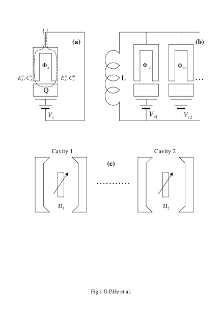
The charge qubits in Josephson junctions. The systems we considered are shown in Fig. 1. A single Josephson-junction qubit consists of a superconducting electron box formed by a symmetric superconducting quantum interference device (SQUID) with Josephson couplings , pierced by a magnetic flux and subject to an applied gate voltage [ is the offset charge, see Fig.1(a)]. In the charging regime [where with being the single-electron charging energy] and at low temperatures, the system behaves as an artificial spin-1/2 particle in a magnetic field, and the Hamiltonian may be expressed as Josephson
| (1) |
where with is a tunable effective Josephson coupling parameter, whose value can be controlled by external flux . are the Pauli matrices. In Eq.(1), we have chosen that charge states and (here is the number of excess Cooper-pair charges on the box) correspond to spin basis states and , respectively. A series of such qubits may be coupled through an inductor [see Fig.1(b)]. An effective interaction is given byJosephson
| (2) |
where and is the -component of Pauli matrices of the th qubit. Then the total Hamiltonian of the system is equivalent to
| (3) |
where , , and . It is worth pointing out that all parameters in Eq. (3) are experimentally controllable by external classical variables and . Thereby, any entangled state as well as single qubit gates required in Bell’s experiment is feasible.
The preparation of a pair of entangled qubits. For simplicity, but without loss of generality, we consider the two-qubit case. By taking , for each single Josephson qubit, and , the Hamiltonian may be rewritten as
| (4) |
The exact solution may be obtained when parameters and are time-independent. Note that any entangled state may be generated even if the initial state is a product state. For example, in terms of computational basis , with the initial state being chosen as , the state of the system at time is found to be
| (5) |
where . Besides, when , (, are both integers and ), we have
| (6) |
This is the maximally entangled state for a pair of qubits [as the concurrence of this state defined in Eq. (17) below is ], and thus, four Bell’s states may be derived from it by simply rotating one of the qubits. In the following discussions we assume in Eq. (5) as our starting point for the test.
The entanglement between two distant Josephson junction qubits may be created by the cavity quantum electrodynamic (QED) techniques. A simple configuration of quantum transmission between two nodes consists of two Josephson charge qubits and which are strongly coupled to their respective cavity modes with the same frequency , as shown in Fig. 1(c). The Hamiltonian describing the interaction of the qubit with the cavity mode isZhu
| (7) | |||||
where and are the creation and annihilation operators, respectively, for cavity mode , , and is the coupling constant between the junctions and the cavity. Based on this kind of coupling and following the method described in Ref. Cirac , we may transfer the quantum state in one qubit to another separated far away. Moreover, by using quantum repeatersBriegel , any long-distance entanglement may be realized, at least in principle. Therefore, a possible scenario to generate an entangled state of long-distant qubits required by nonlocally testing Bell’s inequality is as follows: we may first create an initial entangled state [as Eq. (5)] of two charge qubits in one node, and then transfer the state of one of the pair to another node by the cavity QED technique.
A universal set of single-qubit gates is feasible in the systems. The coupling between charge qubits should be switched off by setting in single-qubit gates. Parameters and in Eq.(1) are experimentally controllable. By assuming and time-independent, the evolution operator is derived as
| (8) |
with . Similarly, by assuming and time-independent, we have
| (9) |
with . The gates described by Eqs.(8) and (9) are a well-known universal set of single-qubit gates: any unitary rotation can be decomposed into a product of successive gates in this set. The gates described by Eqs.(8) and (9) may be referred to as dynamic gatesZhu_pra2003 . It is worth pointing out that a universal set of quantum gates in this system may also be realized by using pure geometric phasesZhu_prl2002 .
The detection method. The population of qubits in states or may be experimentally measured by the dc currents through the probe junctionsNakamura . Putting a probe junction in each qubit, as described in Ref.Nakamura , the measurable dc currents through the probe junction are generated by the following process: emits two electrons to the probe, while does nothing. Consequently, a classical property with two possible outcomes as required by Bell’s experiments, may be detected. The advantage of the above detection technique lies in that a measured outcome may be recorded for every experiment, thereby closing the detection loophole in the same experiment.
All in all, the three basic ingredients required by CHSH type Bell’s experiment are, in principle, feasible in superconducting nanocircuits presented here.
III Testing Bell’s inequality
The detection method addressed above provides a convenient way to experimentally measure the population of the Josephson qubit in state or , and hence is sufficient for testing the Bell inequalityBrif . We show here that the CHSH combinationClauser can be presented by a useful phase-space distribution function Q for the qubits, which can be calculated through the probabilities of finding certain qubits in state or . Assuming that two distant qubits described by Eq. (5) have been created, and each qubit can be manipulated by unitary operators in Eqs.(8) and (9), a new state given by
| (10) |
is derived by rotating separately each qubit in describe by Eq. (5). Evolution operator with a unit vector and denoting qubit . When measuring state , the probability to find the th qubit in state is
| (11) |
and the probability to find both qubits in state is
| (12) |
On the other hand, we may write
which can be understood as the qubit state in the phase space. Then we find that Eq.(11) can be rewritten as
| (13) |
which is just the Q function for the th qubit, where denotes the reduced density matrix of the th qubit. Equation (12) can also be rewritten as
| (14) |
which is just the joint Q function for the system of two qubits. Thus the CHSH combination is given by Brif ; Banaszek
| (15) | |||||
which must satisfy inequality for local theories.
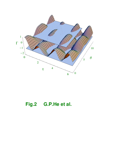
We now consider a two-qubit system. Substituting the state described by Eq.(5) into Eq. (15), we have
| (16) | |||||
For simplicity, but without loss of generality, we here have chosen for and in the calculation. In Fig.2, we plot as a function of and when and . It is seen clearly that the violation of Bell’s inequality for both and may appear in this system. In fact, with other choices for parameters , , , and , function will still have a similar shape and the violation can easily be found. Therefore, the system presented here may be a promising candidate for testing Bell’s inequality.
IV Measuring the entanglement of formation
On the other hand, it is well-known that Bell’s inequality is not very efficient for demonstrating nonlocality, and a better parameter to characterize nonlocality should be the amount of entanglement. Thus it is also highly desirable to develop a feasible method to measure the latter. We now show that the entanglement based on concurrence can also be represented by the phase-space Q function and thus can be experimentally detected.
If we write a state in the form as
then concurrence of state is defined asWootters
| (17) |
and the amount of entanglement can be expressed as
| (18) | |||||
Substituting Eq. (5) into Eq. (17), the concurrence of the state in Eq. (5) is derived as
| (19) | |||||
Let , , and denote the four probabilities associated with outcomes (, , , and ) when measuring and , and , , , and denote the four corresponding probabilities when measuring and . The concurrence in Eq.(17) is found to satisfyentangle
| (20) |
with
The concurrence of a pure two-qubit state may be measured by detection of the Q function defined in Eqs.(11) and (12) since all variables in Eq. (20) are determined by them. By choosing
which correspond to
we find that the probabilities appeared in Eq.(20) are related to the Q function by
Thus the concurrence as well as the amount of entanglement can be deduced by detecting the probabilities of qubits in state .
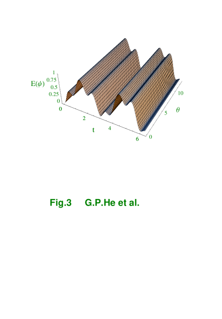
A theoretical result for the amount of entanglement calculated from Eq.(19) is plotted in Fig.3. We can see that does not dependent on . This illustrates that unlike the violation of the Bell’s inequality, the entanglement will not be affected by local transformations. Therefore, the amount of entanglement for the states given by Eqs.(5) and (10) are the same. This also implies that in the sense of characterization of the nonlocal properties, the amount of entanglement defined by Eq. (18) is better than the CHSH combination described by Eq. (15). Thus it is desirable to work out a feasible method to measure the amount of entanglement.
V Conclusions
In conclusion, we proposed a scheme to test Bell’s inequality and to measure the entanglement of two charge qubits in superconducting nanocircuits. We demonstrated that the parameters for these experiments are determined from the Q functions in phase space, which can be measured by the dc currents through the probe junctions. The outcome for every experiment may be recorded, and thus the issue of detection efficiency is replaced by detecting accuracyRowe . By using the cavity QED technique, the entangled state of two charge qubits separated far away may be created. Consequently, it is quite possible that both of the locality loophole and the efficiency loophole can be closed in the same experiment proposed here.
Finally, we wish to make a few remarks on the difficulties of experimental implementation of the scheme. (1) Designing the cavity QED to couple the charge qubits is necessary. The entanglement between two charge qubits was demonstrated in a recent experimentPashkin , and a few quantum phenomena, such as stimulated emission and amplification in Josephson junction arrays within the same high-Q oscillators, were also reported Barbara . However, it is still awaited to make the entangled state between the charge qubit and the single cavity mode. (2) The distance between two cavities is enforced by the strict relativistic separation. Since the measurement time is ns in the experiment reported in Ref.Pashkin or may, in principle, be even shorter with one order of the magnitudeJosephson , it is estimated that the two cavities would have to be physically separated by , which can be realized with current technology if the cavities are connected by a (microwave) transmission fibreZhu ; Cirac ; the transmission of entangled state with the distance of a few kilometers was already realized in quantum telepotationMarcikic . However, it is still very subtle and challenging to couple the (microwave) fibre to the cavity QED experimentally.
VI Acknowledgments
This work was supported in part by the RGC grant of Hong Kong under Grant No. HKU7114/02P and the URC fund of HKU. G. P. H. was supported in part by the NSF of Guangdong Province under Contract No. 011151 and the Foundation of Zhongshan University Advanced Research Centre under Contract No. 02P2. S. L. Z was supported in part by SRF for ROCS, SEM, the NSF of Guangdong province under Grant No. 021088, and the NNSF of China under Grant No. 10204008.
References
- (1) J. S. Bell, Physics (Long Island City, NY) 1, 195 (1964).
- (2) A. Einstein, B. Podolsky, and N. Rosen, Phys. Rev. 47, 777 (1935).
- (3) A. Aspect, P. Grangier, and G. Roger, Phys. Rev. Lett. 49, 91 (1982).
- (4) Y. H. Shih and C. O. Alley, Phys. Rev. Lett. 61, 2921 (1988).
- (5) Z. Y. Ou and L. Mandel, Phys. Rev. Lett. 61, 50 (1988).
- (6) W. Tittel, J. Brendel, H. Zbinden, and N. Gisin, Phys. Rev. Lett. 81, 3563 (1998).
- (7) G. Weihs, T. Jennewein, C. Simon, H. Weinfurter, and A. Zeilinger, Phys. Rev. Lett. 81, 5039 (1998).
- (8) M. A. Rowe, D. Kielpinski, V. Meyer, C. A. Sackett, W. M. Itano, C. Monroe, and D. J. Wineland, Nature (London) 409, 791 (2001).
- (9) A. Aspect, Nature (London) 398, 189 (1999).
- (10) P. Grangier, Nature (London) 405, 774 (2001).
- (11) J. F. Clauser, M. A. Horne, A. Shimony, and R. A. Holt, Phys. Rev. Lett. 23, 880 (1969).
- (12) Y. Makhlin, G.Schön, and A. Shnirman, Nature (London) 398, 305 (1999); Rev. Mod. Phys. 73, 357 (2001)
- (13) Y. Nakamura, Yu. A. Pashkin, and J. S. Tsai, Nature (London) 398, 786 (1999).
- (14) Yu, A. Pashkin, T. Yamamoto, O. Astafiev, Y. Nakamura, D. V. Averin, and J. S. Tsai, Nature (London) 421, 823 (2003).
- (15) S. L. Zhu and Z. D. Wang, Phys. Rev. Lett. 89, 097902 (2002); ibid. 89, 289901(E) (2002); Phys. Rev. A 66, 042322 (2002).
- (16) S. L. Zhu, Z. D. Wang, and K. Yang, Phys. Rev. A (in press); e-print quant-ph/0304173.
- (17) N. D. Mermin, Phys. Rev. Lett. 65, 1838 (1990).
- (18) D. M. Greenberger, M. A. Horne, and A. Zeilinger, in Bell’s Theorem, Quantum Theory and Conceptions of the Universe, edited by M. Kafatos (Kluwer Academic, Dordrecht, 1989), p. 69.
- (19) C. Capasso, D. Fortunato, and F. Selleri, Int. J. Mod. Phys. A 7, 319 (1973); L. Hardy, Phys. Rev. Lett. 71, 1665 (1993).
- (20) J. I. Cirac, P. Zoller, H. J. Kimble, and H. Mabuchi Phys. Rev. Lett. 78, 3221 (1997); S. J. van Enk, J. I. Cirac, and P. Zoller, ibid. 78, 4293 (1997).
- (21) H. J. Briegel, W. Dür, J. I. Cirac, and P. Zoller, Phys. Rev. Lett. 81, 5932 (1998).
- (22) S. L. Zhu and Z. D. Wang, Phys. Rev. A 67, 022319 (2003).
- (23) C. Brif and A. Mann, Europhys. Lett. 49, 1 (2000).
- (24) K. Banaszek and K. Wodkiewicz, Phys. Rev. Lett. 82, 2009 (1999).
- (25) W. K. Wootters, Phys. Rev. Lett. 80, 2245 (1998).
- (26) J. M. G. Sancho and S. F. Huelga, Phys. Rev. A 61, 042303 (2000).
- (27) P. Barbara, A. B. Cawthorne, S. V. Shitov, and C. J. Lobb, Phys. Rev. Lett. 82, 1963 (1999).
- (28) I. Marcikic, H. de Riedmatten, W. Tittel, H. Zbinden, and N. Gisin, Nature (London) 421, 509 (2003).