Theory of quantum Loschmidt echoes

Abstract

In this paper we review our recent work on the theoretical approach to quantum Loschmidt echoes, i.e. various properties of the so called echo dynamics – the composition of forward and backward time evolutions generated by two slightly different Hamiltonians, such as the state autocorrelation function (fidelity) and the purity of a reduced density matrix traced over a subsystem (purity fidelity).

Our main theoretical result is a linear response formalism, expressing the fidelity and purity fidelity in terms of integrated time autocorrelation function of the generator of the perturbation. Surprisingly, this relation predicts that the decay of fidelity is the slower the faster the decay of correlations. In particular for a static (time-independent) perturbation, and for non-ergodic and non-mixing dynamics where asymptotic decay of correlations is absent, a qualitatively different and faster decay of fidelity is predicted on a time scale $\propto 1/\delta$ as opposed to mixing dynamics where the fidelity is found to decay exponentially on a time-scale $\propto 1/\delta^{2}$, where $\delta$ is a strength of perturbation. A detailed discussion of a semi-classical regime of small effective values of Planck constant $\hbar$ is given where classical correlation functions can be used to predict quantum fidelity decay. Note that the correct and intuitively expected classical stability behavior is recovered in the classical limit $\hbar\to 0$, as the two limits $\delta\to 0$ and $\hbar\to 0$ do not commute. The theoretical results are demonstrated numerically for two models, the quantized kicked top and the multi-level Jaynes Cummings model. Our method can for example be applied to the stability analysis of quantum computation and quantum information processing.

1 Introduction

In the early days of statistical mechanics, J. Loschmidt in a discussion with L. Boltzman suggested to study irreversibility by changing the velocities of all the molecules in a box which are, after an equal amount of time, supposed to return to their initial positions. Since the discovery of deterministic chaos, however, we know that such a gedanken experiment won’t work after a short while since typical systems of many particles possess exponentical sensitivity on the variation of initial condition. Therefore arbitrarily small but non-vanishing perturbation of the trajectory (i.e. initial condition), or perturbation of the equations of motion (e.g. introducing a small external force field like gravity), drive the returning orbit away and hence the orbit will never return to the initial phase space point. Both mechanisms, namely perturbing the initial condition or perturbing the Hamiltonian, produce a similar effect in classical mechanics.

This, however, is not the case in quantum mechanics. Due to manifest linearity and unitarity of quantum equation of motion (Schrödinger equation), quantum dynamics is always stable against small variations of the initial state described by the wave-function [1]. Yet small variation in the Hamiltonian can produce interesting and highly non-trivial effects on quantum time evolution.

It has been suggested by A. Peres [2, 3] that susceptibility of quantum evolution to small system variations, as measured by the Fidelity $F(t)=|\langle\psi(t)|\psi_{\delta}(t)\rangle|^{2}$ of the states of the perturbed $|\psi_{\delta}(t)\rangle$ and unperturbed $|\psi(t)\rangle$ time evolution, can provide a useful signature of classical chaos in quantum motion. Peres suggested that classically chaotic systems are characterized by fast exponential decay of fidelity $F(t)$, while the decay in regular systems should be qualitatively slower. This conclusion was asserted, based on a numerical experiment where an initial coherent state has been placed, respectively, inside the chaotic region of classical phase space, or in the middle of KAM island of classically regular motion. This view, elaborated semiclassically by Jalabert and Pastawski [4] in the regime of initial coherent states and very short time scale, i.e. shorter than the so-called Ehrenfest time $t_{\rm E}\propto-\log\hbar$ [5], is consistent with a semiclassical picture of decoherence of Zurek [6], which predicts, in the same semiclassical regime, that von Neumann entropy of a reduced density matrix of a central system traced over the environment grows with the rate proportional to the classical Lyapunov exponent (or better to say, local classical phase space stretching rate). According to this picture, fidelity decays exponentially $F(t)\propto\exp(-\lambda t)$ for classically chaotic systems, with the perturbation independent rate $\lambda$ which matches the local classical phase-space stretching rate.

We stress that this picture is justified under two rather severe assumptions: (i) coherent initial states which allow quantum-classical correspondence in phase space and (ii) short-times $t<t_{\rm E}$ which guarantee pointwise quantum-classical correspondence of time evolution. If either of the two conditions is broken, the above picture can be shown to be incorrect [7]. In quantum information processing, in particular, one is certainly not interested in processing coherent initial states but rather random initial states which contain a maximal amount of quantum information. Furthermore, one is interested in the behaviour of fidelity $F(t)$ for asymptotically long times, certainly longer than the Ehrenfest barrier $t_{\rm E}$.

In a series of papers [8, 9, 7, 10, 11, 12] we have elaborated on a linear response approach to fidelity decay which allows to deduce the behaviour of $F(t)$ in the entire range of times for sufficiently small perturbation strength. In several cases linear response (perturbative) results can be extended to include all-orders in perturbation parameter and yield asymptotic long-time tails of $F(t)$. The central result of this work is a linear-response fluctuation-dissipation formula which expresses fidelity $F(t)$ in terms of integrated time-correlation function of the perturbation. As a general consequence of this formula, it follows that stronger correlation decay (typically associated with stronger classical chaos of the underlying classical counterpart) means higher fidelity, or slower decay of fidelity. This has been quite an unexpected result as it seems just oposite to the short-time semiclassical picture [4]. However it can be shown, as a consequence of a delicate competition of time-scales (see e.g. Ref.[7] or the present paper), that the two pictures are not contradictory but they’re in fact complementary, and that there is a crossover of fidelity decay $F(t)$ at $t\sim t_{\rm E}$ from classical to quantum behaviour.

Fidelity decay is sometimes associated with decoherence, which is a dynamical property of open quantum system coupled to another quantum system interpreted as environment. In order to elucidate this from a dynamical point of view, we have introduced [10, 11, 12] a novel concept of purity fidelity, namely the purity of a reduced density matrix of a central system traced over the environment (or another part of a system) after undergoing the (Loschmidt) echo dynamics. We show an intimate relationship between purity fidelity and fidelity decay, and develop a linear response theory for purity fidelity in terms of special time-correlation functions of the generator of perturbation.

This paper is a short comprehensive review of theoretical results on fidelity and purity fidelity which appeared in a series of recent papers [8, 9, 7, 10, 11, 12]. Beyond that we discuss important aspects which have not yet been considered before, such as the case of coherent initial states, regular classical dynamics and ‘ergodic’ perturbation with vanishing time-average.

It should be noted that a considerable recent interest in quantum Loschmidt echoes [4, 8, 9, 7, 10, 11, 12, 13, 14, 15, 16, 17, 18, 19] has been largely stimulated by spin echo experiments performed by the group of H. Pastawski [20], and that fidelity is used as a benchmark for the quantum information processes.[21]

2 General theory of fidelity: linear response and beyond

Let us consider a unitary operator $U$ being either (i) a short-time propagator $U=\exp(-iH\Delta/\hbar)$ generated by some time-independent Hamiltonian $H$, or (ii) a Floquet map $U=\hat{\cal T}\exp(-i\int_{0}^{p}d\tau H(\tau)/\hbar)$ of periodic time-dependent Hamiltonian $H(\tau+p)=H(\tau)$. Arbitrary time evolution is generated by a group $U^{t}$ where integer $t$ is a discrete time variable. Note that in the continuous time case (i) we may let $\Delta\to 0$, so $\tau=t\Delta$ becomes a continuous time variable. Thus we shall consider the case of discrete time and develop general formalism for that case, whereas in the end the formulae for continuous time shall simply be obtained as the limit $\Delta\to 0$.

A general (static, for time dependent case see Ref.[9]) small perturbation of unitary propagator $U$ can be ‘parametrized’ in terms of some bounded hermitian operator $V$ as

$$U_{\delta}=U\exp(-iV\delta/\hbar),$$ (1)

where $\delta$ is a small strength parameter. We note that $V$ corresponds to the perturbation of the Hamiltonian $H_{\delta}=H+\delta V$ in the continous time limit $\Delta\to 0$. We also want to keep dependences on the (effective) Planck constant $\hbar$ explicit so we can control the semiclassical behaviour. For systems with a well defined semiclassical limit we shall be interested in the perturbations $V$ which have well defined classical limit or Weyl symbol $v({\bm{q}},{\bm{p}})$.

Starting from some initial reference state $|\psi\rangle$, we consider two quantum time evolutions $|\psi(t)\rangle=U^{t}|\psi\rangle$, $|\psi_{\delta}(t)\rangle=U^{t}_{\delta}|\psi\rangle$, and investigate a distance between the resulting Hilbert states as measured by fidelity $F(t)=|\langle\psi_{\delta}(t)|\psi(t)\rangle|^{2}$. It is crucial to note that fidelity can be written in terms of expectation value $\langle\bullet\rangle=\langle\psi|\bullet|\psi\rangle$ of the unitary echo operator

$$M_{\delta}(t)=U^{-t}_{\delta}U^{t},$$ (2)

namely

$$F(t)=|\langle M_{\delta}(t)\rangle|^{2}.$$ (3)

We shall later discuss the dependence of fidelity on dynamical properties of the time-evolution $U$, on the strength of perturbation $\delta$, and on the structure of initial state $|\psi\rangle$.

Concerning the last point it is often useful to study fidelity with respect to a random initial state $|\psi\rangle$, i.e. to average, denoted by $\langle\!\langle\bullet\rangle\!\rangle$, over an ensemble of initial states with a unitarily invariant measure in $N$-dimensional Hilbert space. This should generally correspond to processing of states with maximal quantum information (entropy) which is certainly the situation of most interest for quantum computation [21]. We note that bilinear expressions in $|\psi\rangle$ are averaged by means of a trace,

$$\langle\langle\psi|A|\psi\rangle\rangle_{\psi}=:\langle\!\langle A\rangle\!\rangle=\frac{1}{\cal N}\,{\rm tr}\,A,$$ (4)

however higher order expressions, like fidelity (3) which is of fourth order in random variable $|\psi\rangle$, have to be averaged by means of pair contractions in the asymptotic Gaussian (${\cal N}\to\infty$) limit. For example, one can compute the average fidelity $\langle\!\langle F(t)\rangle\!\rangle$ in terms of the average fidelity-amplitude $\langle\!\langle f(t)\rangle\!\rangle=\langle\!\langle M_{\delta}(t)\rangle\!\rangle$ with a small, semiclassically vanishing correction

$$\langle\!\langle F(t)\rangle\!\rangle=\left|\langle\!\langle f(t)\rangle\!\rangle\right|^{2}+\frac{1}{\cal N}.$$ (5)

Thus we have shown that the variation of fidelity with respect to random initial states becomes unimportant for large Hilbert space dimensions ${\cal N}$, e.g. when approaching either the semiclassical or the thermodynamic limit, so one is justified to average the amplitude $f(t)$ in order to simplify theory.[7]

On the other hand, for the purpose of quantum classical correspondence, it is most suitable to consider coherent initial states $|\psi\rangle$, in some sense the states of ‘minimal quantum information’. Below we shall specify our general formulae for the two extremal cases, namely random and coherent initial states.

To derive our general theory we first rewrite the echo operator (2) in terms of a time-dependent perturbation operator in the interaction picture

$$V_{t}:=U^{-t}VU^{t}.$$ (6)

Then we recursively insert the expression of unity $\mathbbm{1}=U^{t^{\prime}}U^{-t^{\prime}}$ in the definition (2) and observe $U^{-t^{\prime}}U_{\delta}^{-1}U^{1+t^{\prime}}=\exp(iV_{t^{\prime}}\delta/\hbar)$ for $t^{\prime}$ running from $t-1$ downto $0$, yielding

$$M_{\delta}(t) = U_{\delta}^{-t}U^{t}=U_{\delta}^{-(t-1)}U^{t-1}U^{-(t-1)}(U_{\delta}^{-1}U)U^{t-1}=$$ (7)

$$= U_{\delta}^{-(t-1)}U^{t-1}\exp(iV_{t-1}\delta/\hbar)=$$

$$= U_{\delta}^{-(t-2)}U^{t-2}\exp(iV_{t-2}\delta/\hbar)\exp(iV_{t-1}\delta/\hbar)=$$

$$\ldots$$

$$= \exp(iV_{0}\delta/\hbar)\exp(iV_{1}\delta/\hbar)\cdots\exp(iV_{t-1}\delta/\hbar).$$

The obvious next step is to expand the product (7) into a power-series in $\delta$

$$M_{\delta}(t)=\mathbbm{1}+\sum_{m=1}^{\infty}\frac{i^{m}\delta^{m}}{m!\hbar^{m}}\hat{\cal T}\!\!\!\sum_{t_{1},\ldots,t_{m}=0}^{t-1}V_{t_{1}}V_{t_{2}}\cdots V_{t_{m}},$$ (8)

where the operator $\hat{\cal T}$ denotes a left-to-right time ordering. Such a perturbative expansion converges absolutely for any $\delta$ provided that the perturbation $V$ is a bounded operator. Therefore fidelity may be computed to arbitrary order in $\delta$ by truncation of the above expansion (8) and plugging it into (3). So we can see that the fidelity $F(t)$ can be expressed entirely in terms of multiple time correlation functions of the generator $V$ of the perturbation.

To second order in $\delta$ one obtains a very useful linear response formula

$$F(t)=1-\frac{\delta^{2}}{\hbar^{2}}\sum_{t^{\prime},t^{\prime\prime}=0}^{t-1}C(t^{\prime},t^{\prime\prime})+{\cal O}(\delta^{3}),$$ (9)

where

$$C(t^{\prime},t^{\prime\prime}):=\langle V_{t^{\prime}}V_{t^{\prime\prime}}\rangle-\langle V_{t^{\prime}}\rangle\langle V_{t^{\prime\prime}}\rangle$$ (10)

is a 2-point time correlation function of the quantum observable $V$. This formula can be interpreted in terms of a dissipation-fluctuation relationship. On the LHS we have fidelity which describes dissipation of quantum information and on the RHS we have an integrated time-correlation function (fluctuation). A simple-minded qualitative conclusion drawn from the formula (9) says: The stronger the decay of correlations the slower the decay of fidelity and vice versa. The linear response formula can be rewritten in a slightly more compact notation as

$$F(t)=1-\frac{\delta^{2}}{\hbar^{2}}C_{\rm int}(t),$$ (11)

where

$$C_{\rm int}(t)=\langle\Sigma(t)^{2}\rangle-\langle\Sigma(t)\rangle^{2},\quad\Sigma(t)=\sum_{t^{\prime}=0}^{t-1}V_{t^{\prime}}.$$ (12)

We shall use this compact notation later in section 3.

Note that the range of validity of the above formula (9,11) is not at all restricted to short times. The only condition is that $\delta$ is sufficiently small such that $1-F(t)$ is small ($\ll 1$). Below we shall discuss different regimes and different time-scales based on this formula and its higher order extensions. In the semiclassical regime of approaching the classical limit $\hbar\to 0$ the quantum correlation function $C(t^{\prime},t^{\prime\prime})$ goes over to the corresponding correlation function of the classical perturbation $v({\bm{q}}(t),{\bm{p}}(t))$.

Therefore the fidelity for classically chaotic systems will decay with the rate which is inversely proportional to their rate of mixing. Furthermore for classically non-ergodic, i.e. regular or integrable motion, the correlation functions will generally not decay to zero and the fidelity will therefore decay much faster.

For continuous time $t$ one expects that in the so-called Zeno regime of short times, such that correlation function does not yet decay appreciably. Fidelity will always decay quadratically $F(t)\approx 1-\delta^{2}C(0)t^{2}/\hbar^{2}$. This is independent of the nature of the corresponding classical dynamics, whether it is regular or chaotic. However we are interested in longer times, beyond the range of quantum Zeno dynamics.

2.1 Regime of ergodicity and fast mixing

Here we assume that the system is (classically) ergodic and mixing such that the correlation function $C(t^{\prime},t^{\prime\prime})$ decays sufficiently fast as $|t^{\prime}-t^{\prime\prime}|$ grows; this typically corresponds to globally chaotic classical motion. This also implies that after a certain short (Ehrenfest) time scale $t_{\rm E}$, which can for a chaotic system be written $t_{\rm E}\approx\log(1/\hbar)/\lambda$ in terms of an effective classical Lyapunov exponent $\lambda$, the time correlation functions become independent of the initial state and thus equal to the random state average, e.g.

$$C(t,t+\tau)=C(\tau):=\langle\!\langle VV_{\tau}\rangle\!\rangle,\quad{\rm if}\quad t\gg t_{\rm E}.$$ (13)

In this situation we can safely assume random initial states, or argue that for times larger than $t_{E}$ the results are the same for any inital state. Then the linear response formula can be rewritten as

$$\langle\!\langle F(t)\rangle\!\rangle=1-\frac{2\delta^{2}}{\hbar^{2}}\left\{\frac{1}{2}tC(0)+\sum_{t^{\prime}=1}^{t-1}{(t-t^{\prime})C(t^{\prime})}\right\}+{\cal O}(\delta^{3}).$$ (14)

Now we shall assume that correlation function $C(t)$ decays sufficiently fast, i.e. faster than ${\cal O}(t^{-1})$ and that a certain effective time-scale $t_{\rm mix}$ of decay of $C(t)$ exist. For times $t\gg t_{\rm mix}$ we can neglect the second term under the summation in (14) and obtain a linear decay in time $t$ in the linear response regime

$$F_{\rm em}(t)=1-2(\delta/\hbar)^{2}\sigma t\qquad{\rm with}\qquad\sigma=\frac{1}{2}C(0)+\sum_{t=1}^{\infty}{C(t)}.$$ (15)

Here, $\sigma$ plays the role of a transport coefficient.

We can make a stronger statement valid beyond the linear response regime if we make an additional assumption on the factorization of higher order time-correlations, namely that of $n-$point mixing. This implies that $2m$-point correlation $\langle\!\langle V_{t_{1}}\cdots V_{t_{2m}}\rangle\!\rangle$ is appreciably different from zero for $t_{2m}-t_{1}\to\infty$ only if all the (ordered) time indices $\{t_{j},j=1\ldots 2m\}$ are paired with the time differences within each pair $t_{2j}-t_{2j-1}$ being of the order or less than $t_{\rm mix}$. Here we have assumed without loss of generality that the perturbation is traceless $\langle\!\langle V\rangle\!\rangle=0$. If not, we subtract $\langle\!\langle V\rangle\!\rangle\mathbbm{1}$ from $V$ which does not affect probability $F(t)$. Then we can make a further reduction, namely if $t\gg mt_{\rm mix}$

$$\!\hat{\cal T}\!\!\!\!\!\sum_{t_{1},\ldots,t_{2m}=0}^{t-1}\!\!\!\!\langle\!\langle V_{t_{1}}V_{t_{2}}\cdots V_{t_{2m}}\rangle\!\rangle\rightarrow\hat{\cal T}\!\!\!\!\!\sum_{t_{1},\ldots,t_{2m}=0}^{t-1}\!\!\!\!\langle\!\langle V_{t_{1}}V_{t_{2}}\rangle\!\rangle\cdots\langle\!\langle V_{t_{2m-1}}V_{t_{2m}}\rangle\!\rangle\rightarrow\frac{(2m)!}{m!}(t\sigma)^{m}.\!\!\!\!\!\!\!\!\!\!\!$$ (16)

We then obtain a global exponential decay

$$F_{\rm em}(t)=\left|\langle\!\langle M_{\delta}(t)\rangle\!\rangle\right|^{2}=\exp{(-2t/\tau_{\rm em})},\qquad\qquad\tau_{\rm em}=\frac{\hbar^{2}}{\delta^{2}\sigma},$$ (17)

with a time-scale $\tau_{\rm em}={\cal O}(\delta^{-2})$. We should stress that the above result (17) has been derived under the assumption of true quantum mixing [22], which can be justified only in the limit ${\cal N}\rightarrow\infty$, e.g. either in semiclassical or thermodynamic limit where the correction (5) is irrelevant. Note that the result (17) can be connected to Fermi golden rule [13] as it is based on time-dependent perturbation theory.

2.2 Non-mixing and non-ergodic regime

The opposite situation of non-mixing and non-ergodic quantum dynamics, which typically corresponds to integrable, near-integrable (KAM), or mixed classical dynamics, is characterized by a non-vanishing time-average of the correlation function

$$\bar{C}=\lim_{t\to\infty}{\frac{1}{t^{2}}\sum_{t^{\prime},t^{\prime\prime}=0}^{t-1}C(t^{\prime},t^{\prime\prime})}.$$ (18)

Here, due to non-ergodicity, the time-average $\bar{C}$ depends on the structure of the initial state $|\psi\rangle$. We further assume that a certain characteristic averaging time-scale $t_{\rm ave}$ exists, namely it is an effective time $t=t_{\rm ave}$ at which the limiting process (18) converges. Therefore, for sufficiently large times $t\gg t_{\rm ave}$, the double sum on RHS of eq. (9) can be approximated as $\bar{C}t^{2}$, so the linear-response formula (9) yields, in contrast to (15), a quadratic decay in time

$$F_{\rm ne}(t)=1-\left(\frac{t}{\tau_{\rm ne}}\right)^{2}+{\cal O}(\delta^{3}),\qquad\tau_{\rm ne}=\frac{\hbar}{\delta\sqrt{\bar{C}}},$$ (19)

with time-scale $\tau_{\rm ne}={\cal O}(\delta^{-1})$. One should observe that the non-ergodic time-scale $\tau_{\rm ne}$ can be much smaller than the ergodic-mixing time-scale $\tau_{\rm em}$ (17) provided $\hbar$ is fixed, or the limit $\delta\to 0$ is taken prior to the limit $\hbar\to 0$. Yet $\tau_{\rm ne}$ is typically still much longer than the Zeno time scale of universal quadratic decay.

Again we can make a much stronger general statement going beyond the second order $\delta$-expansion. If we assume that $t\gg t_{\rm ave}$, we can re-write the $m$-tuple sums in the series (8) in terms of a time average perturbation operator

$$\bar{V}=\lim_{t\to\infty}{(1/t)\sum_{t^{\prime}=0}^{t-1}{V_{t^{\prime}}}},$$ (20)

namely

$$f_{\rm ne}(t)=\sum_{m=0}^{\infty}{\frac{(i\delta t)^{m}}{\hbar^{m}m!}\langle\bar{V}^{m}\rangle}=\langle\exp{(it\bar{V}\delta/\hbar)}\rangle,\quad F_{\rm ne}(t)=|f_{\rm ne}(t)|^{2}.$$ (21)

Note that $\bar{V}$ is by construction an integral of motion [23], $[U,\bar{V}]\equiv 0$, and reduces to a trivial multiple of identity in the case of ergodic dynamics studied in previous subsection. Whereas in an ergodic and mixing case, $m-$th order term of (8) grows with time only as ${\cal O}(t^{m/2})$ (for even $m$) since it is dominated by pair time correlations, here in a non-ergodic case, the non-trivial time average operator $\bar{V}$ already gives the dominant effect, namely ${\cal O}(t^{m})$ for $m-$th order term of (8), so the effect of pair time correlations can safely be neglected for sufficiently long times ($t\gg t_{\rm ave}$). Observe also that time averaged correlation is just a variation of the time averaged perturbation

$$\bar{C}=\langle\bar{V}^{2}\rangle-\langle\bar{V}\rangle^{2}.$$ (22)

In the semiclassical regime for random initial states, $\bar{C}$ goes to a purely classical ($\hbar$-independent) quantity $\bar{C}_{\rm cl}=\langle\bar{v}^{2}\rangle_{\rm cl}-\langle\bar{v}\rangle^{2}_{\rm cl}$ where $\bar{v}$ is a time-averaged classical limit of observable $V$ and $\langle\bullet\rangle_{\rm cl}$ is a classical (microcanonical) phase-space average.

Our conclusions may not be valid in the special case where the time-average $\bar{V}$ is a trivial operator, namely when it either vanishes or is proportional to identity. This can happen for very special choices of perturbations $V$ or for systems and perturbations with particular geometric or algebraic symmetries. This option also implies that the classical time-average is trivial $\bar{v}\equiv{\rm const}$, and that $\bar{C}=0$. Of course, in such a case, fidelity decay has to be discussed separately, see e.g. Refs.[24, 15].

Let us now use expression (21) to derive some explicit semiclassical results in the special case of integrable classical dynamics. For a system with $d$ degrees of freedom we thus have $d$ canonical constants of motion – the action variables ${\bm{I}}=(I_{1},\ldots,I_{d})$, which are quantized using EBK rule ${\bm{I}}_{\bm{n}}=\hbar({\bm{n}}+{\bm{\gamma}}/4)$ where ${\bm{n}}=(n_{1},\ldots,n_{d})$ is a vector of integer quanum numbers $n_{j}$ and ${\bm{\gamma}}=(\gamma_{1},\ldots,\gamma_{d})$ is a vector of integer Maslov indices $\gamma_{j}$; the latter are irrelevant for the discussion that follows. Since the time averaged operator $\bar{V}$ commutes with $U$ and with the actions ${\bm{I}}$, it is diagonal in the (generically non-degenerate) basis of eigenstates of ${\bm{I}}$ (quantized tori) $|{\bm{n}}\rangle$. In leading semiclassical order one may write

$$\langle{\bm{n}}|\bar{V}|{\bm{n}}^{\prime}\rangle=\delta_{{\bm{n}},{\bm{n}}^{\prime}}\bar{v}({\bm{I}}_{\bm{n}})$$ (23)

where $\bar{v}({\bm{I}})$ is the corresponding classical time-averaged observable in action space. The fidelity (21) can therefore be written as

$$f_{\rm ne}(t)=\sum_{{\bm{n}}}\exp(it\bar{v}({\bm{I}}_{\bm{n}})\delta/\hbar)|\langle{\bm{n}}|\psi\rangle|^{2}.$$ (24)

Provided the diagonal elements of the density matrix can be written in terms of some smooth structure function $D({\bm{I}}_{{\bm{n}}})=|\langle{\bm{n}}|\psi\rangle|^{2}$, and replacing the sum (24) by an integral over the action space, which is justified for small $\hbar$ up to classically long time $\propto\hbar^{0}\delta^{-1}$, we obtain

$$f_{\rm ne}(t)=\hbar^{-d}\int\!d^{d}{\bm{I}}\,\exp{\{it\bar{v}({\bm{I}})\delta/\hbar\}}D({\bm{I}}).$$ (25)

The obvious next step is to compute this integral by a method of stationary phase. However the result depends on the precise form of the function $D({\bm{I}})$ which may in turn depend explicitly on $\hbar$. Below we work out the details for two important special cases, namely a random and a coherent initial state.

2.2.1 Semiclassical asymptotics for a random initial state.

Let us first assume uniform averaging over (random) initial states $D({\bm{I}})\equiv 1/{\cal N}=(2\pi\hbar)^{d}/{\cal V}$. For large $t\delta/\hbar$ the above integral (25) can be written as a sum of contributions stemming from, say $p$ points, ${\bm{I}}_{\eta},\eta=1,\ldots,p$ where the phase is stationary, $\partial\bar{v}({\bm{I}}_{\eta})/\partial{\bm{I}}=0$. This yields

$$f_{\rm ne}^{\rm ave}(t)=\frac{(2\pi)^{3d/2}}{\cal V}\left|\frac{\hbar}{t\delta}\right|^{d/2}\sum_{\eta=1}^{p}\frac{\exp\{it\bar{v}({\bm{I}}_{\eta})\delta/\hbar+i\nu_{\eta}\}}{|\det{\rm\mathbf{\bar{V}}}_{\eta}|^{1/2}},$$ (26)

where $\{{\rm\mathbf{\bar{V}}}_{\eta}\}_{jk}:=\partial^{2}\bar{v}({\bm{I}}_{\eta})/\partial I_{j}\partial I_{k}$ is a matrix of second derivatives at the stationary point $\eta$, and $\nu_{\eta}=\pi(m_{+}-m_{-})/4$ where $m_{\pm}$ are the numbers of positive/negative eigenvalues of the matrix ${\rm\mathbf{\bar{V}}}_{\eta}$. The stationary phase formula (26) is expected to be correct in the range ${\rm const}\,\hbar/\delta<t<{\rm const}^{\prime}/\delta$. Most interesting to note is the asymptotic power-law time and perturbation dependence $F^{\rm ave}_{\rm ne}\sim|\hbar/(t\delta)|^{d}$, which allows for a possible crossover to a Gaussian decay[8] when approaching the thermodynamic limit $d\to\infty$.

2.2.2 Semiclassical asymptotics for a coherent initial state.

Now let us consider a single $d$-dimensional general coherent state centered at $({\bm{I}}^{*},{\bm{\theta}}^{*})$ in action-angle space

$$\langle{\bm{n}}|{{\bm{I}}^{*},{\bm{\theta}}^{*}}\rangle=\left(\frac{\hbar}{\pi}\right)^{d/4}\!\!\!\left|\det\Lambda\right|^{1/4}\exp\left\{-\frac{1}{2\hbar}({\bm{I}}_{{\bm{n}}}-{\bm{I}}^{*})\cdot\Lambda({\bm{I}}_{{\bm{n}}}-{\bm{I}}^{*})-i{\bm{n}}\cdot{\bm{\theta}}^{*}\right\},$$ (27)

where $\Lambda$ is a positive symmetric $d\times d$ matrix of squeezing parameters, giving

$$D({\bm{I}})=(\hbar/\pi)^{d/2}\left|\det\Lambda\right|^{1/2}\exp(-({\bm{I}}-{\bm{I}}^{*})\cdot\Lambda({\bm{I}}-{\bm{I}}^{*})/\hbar)$$ (28)

and

$$f^{\rm coh}_{\rm ne}(t)=\frac{\left|\det\Lambda\right|^{1/2}}{(\pi\hbar)^{d/2}}\int\!d^{d}{\bm{I}}\,\exp\left\{\frac{1}{\hbar}\left(it\bar{v}({\bm{I}})\delta-({\bm{I}}-{\bm{I}}^{*})\cdot\Lambda({\bm{I}}-{\bm{I}}^{*})\right)\right\}.$$ (29)

Using the assumption $\delta t\ll 1$, we see that a unique stationary point ${\bm{I}}_{s}$ of the exponent approaches ${\bm{I}}^{*}$ as $\delta\to 0$,

$${\bm{I}}_{s}={\bm{I}}^{*}-\frac{it\delta}{2}\Lambda^{-1}{\bm{v}}^{\prime}+{\cal O}(\delta^{2}),\quad{\rm where}\quad{\bm{v}}^{\prime}:=\frac{\partial\bar{v}({\bm{I}}^{*})}{\partial{\bm{I}}}$$ (30)

so we may explicitly evaluate (29) by the method of stationary phase without any lower bound on the range of time $t$,

$$f^{\rm coh}_{\rm ne}(t)=\exp\left\{-\frac{({\bm{v}}^{\prime}\cdot\Lambda^{-1}{\bm{v}}^{\prime})\delta^{2}}{4\hbar}t^{2}+\frac{i\bar{v}({\bm{I}}^{*})\delta}{\hbar}t\right\}.$$ (31)

Note that the fidelity decay for a coherent initial state with regular classical motion has a time-scale

$$\tau_{\rm ne-coh}=(2\hbar)^{1/2}({\bm{v}}^{\prime}\cdot\Lambda^{-1}{\bm{v}}^{\prime})^{-1/2}\delta^{-1}\;\;\propto\;\;\hbar^{1/2}\delta^{-1},$$ (32)

which is consistent with (19) with $\bar{C}=\frac{1}{2}\hbar({\bm{v}}^{\prime}\cdot\Lambda^{-1}{\bm{v}}^{\prime})$ and is by a factor proportional to $\hbar^{-1/2}$ longer than the time-scale $\tau_{\rm ne}\propto\hbar/\delta$ for a random initial state. It should be noted that the above derivation of fidelity decay for a coherent initial state (27-32) remains valid in a near-integrable (KAM) situation of mixed classical phase space, provided that the initial wave packet is launched in a regular region of phase space where (local) action-angle variables exist.

2.3 Finite size effects and time and perturbation scales

The theoretical relations of the previous subsections are strictly justified in the asymptotic limit ${\cal N}\to\infty$. For finite ${\cal N}$, fidelity $F(t)$ cannot decay indefinitely but starts to fluctuate for long times due to discreteness of the spectrum of the evolution operator $U$. Let us write the eigenphases of $U$ and $U_{\delta}$, and the corresponding eigenvectors, respectively, as $\phi_{n}$, $\phi^{\delta}_{n}$, and $|\phi_{n}\rangle$, $|\phi^{\delta}_{n}\rangle$, $n=1,\ldots,{\cal N}$, satisfying $U|\phi_{n}\rangle=e^{-i\phi_{n}}|\phi_{n}\rangle$, $U_{\delta}|\phi^{\delta}_{n}\rangle=e^{-i\phi^{\delta}_{n}}|\phi^{\delta}_{n}\rangle$. Now define a unitary operator $W$ which maps the eigenbasis of $U$ to the eigenbasis of $U_{\delta}$, namely $W|\phi_{n}\rangle:=|\phi^{\delta}_{n}\rangle$ for all $n$, with matrix elements $W_{mn}:=\langle\phi_{m}|W|\phi_{n}\rangle$, and write the initial state as $\psi_{n}=\langle\phi_{n}|\psi\rangle$. Note that the matrix $W_{mn}$ is real orthogonal if $U$ and $U_{\delta}$ possess a common anti-unitary symmetry (e.g. time-reversal). Now it is straightforward to rewrite the fidelity amplitude as

$$f(t)=\sum_{l,m,n}\psi^{*}_{n}\psi_{m}W^{*}_{nl}W_{ml}\exp\left(i(\phi_{n}-\phi^{\delta}_{l})t\right),$$ (33)

At this point we are interested in the long time fluctuations so we compute the time averaged fidelity fluctuation

$$F_{\rm ta}:=\lim_{T\to\infty}\frac{1}{T}\int_{0}^{T}dt|f(t)|^{2}=\sum_{k,l,m,n}\psi_{k}^{*}W_{kl}^{*}\psi_{m}W_{ml}|\psi_{n}|^{2}|W_{nl}|^{2}.$$ (34)

In the process of averaging over the time we have assumed that the eigenphases are non-degenerate so $\overline{\exp(i(\phi_{n}-\phi_{n^{\prime}}+\phi^{\delta}_{l}-\phi^{\delta}_{l^{\prime}})t)}=\delta_{nn^{\prime}}\delta_{l,l^{\prime}}$. We see that fidelity fluctuation $F_{\rm ta}$ depends on the orthogonal/unitary matrix $W_{mn}$ and the initial state. Detailed discussion of various cases are given in Ref.[7] Here we only give results for random intitial state, where $\psi_{n}$ can be assumed, for large ${\cal N}$, to be independent complex random Gaussian variables with variance $1/{\cal N}$. Averaging over an ensemble of initial states yields

$$\langle\!\langle F_{\rm ta}\rangle\!\rangle=\frac{1}{{\cal N}^{2}}\left(\sum_{n,l}|W_{nl}|^{4}+\sum_{n,m,l}|W_{nl}|^{2}|W_{ml}|^{2}\right).$$ (35)

For sufficiently weak perturbation, one may assume that the matrix $W_{n,m}$ is near identity $W_{n,m}\approx\delta_{n,m}$, thus $F^{\rm weak}_{\rm ta-ii}=2/{\cal N}$ while for strong perturbation $W_{n,m}$ can be assumed to be a random matrix, yielding $F^{\rm strong}_{\rm ta-ii}=1/{\cal N}$. Therefore the $1/{\cal N}$ dependence of the residual fidelity $F_{\rm ta}$, for random intial states does not depend on the structure of eigenstates $W_{n,m}$, and there is only a factor of $2$ difference between the two extreme cases.

In addition to a random initial state, we shall now assume ergodic and mixing classical dynamics, so fidelity decay is initially given by exponential law (17) until it reaches the plateau (35). The saturation time $t_{*}$ where $F_{\rm em}(t_{*})=F_{\rm ta}$, is the first important time scale

$$t_{*}=\frac{1}{2}\tau_{\rm em}\ln{\cal N}\approx\frac{\hbar^{2}d}{\delta^{2}\sigma_{\rm cl}}\ln(1/\hbar),$$ (36)

where $\sigma_{\rm cl}$ is the classical limit of the transport coefficient (15).

The second new time-scale is related to the asymptotic non-decay of time correlations for finite-${\cal N}$ quantum dynamics, namely even if the system is classically mixing the quantum correlation function will have a small non-vanishing ($\hbar$-dependent) time average

$$\bar{C}=\overline{\langle V(t)V(t^{\prime})\rangle}=\sum_{n}|\psi_{n}|^{2}(V_{nn})^{2},$$ (37)

where $V_{mn}=\langle\phi_{m}|V|\phi_{n}\rangle$. Since, however, the classical system is assumed to be chaotic, implying ergodicity and mixing, the matrix elements $V_{mn}$ behave like pseudo-random variables with a variance given by the Fourier transformation $S(\omega)$ of the corresponding classical correlation function $C_{\rm cl}(t)$ at frequency $\omega=\phi_{m}-\phi_{n}$ [25]. On the diagonal we have $\omega=0$ and an additional factor of $2$ due to the form of the invariant random matrix measure (see e.g. [26]). Thus we have

$$\bar{C}=\frac{4\sigma_{\rm cl}}{\cal N},$$ (38)

where $\sigma_{\rm cl}=S(0)/2$ is the classical limit of (15). The result, due to ergodicity, does not depend on the particular form of the initial state $|\psi\rangle$. The decay of fidelity (14) will start to be dominated by the average plateau (38) at sufficiently long time $t$, when $\sum_{t^{\prime}=0}^{t-1}{(t-t^{\prime})\bar{C}}\approx 2\sigma_{\rm cl}t^{2}/{\cal N}\geq\sigma_{\rm cl}t$, i.e. for times $t$ greater than $t_{\rm p}$

$$t_{\rm p}=\frac{1}{2}{\cal N}\propto\hbar^{-d},$$ (39)

which is just the Heisenberg time associated to the inverse density of states.

Depending on the interrelation among four (or five) time-scales $\tau_{\rm em}\propto\hbar^{2}\delta^{-2}$, $t_{\rm p}\propto\hbar^{-d}\delta^{0}$, $t_{*}\propto\hbar^{2}\ln(1/\hbar)\delta^{-2}d$, $t_{\rm mix}\propto\hbar^{0}\delta^{0}$, (and $t_{\rm E}\propto\ln(1/\hbar)\delta^{0}$ if we are considering coherent initial states, like e.g. [4, 14, 13]) we can have four (or five) different regimes depending on the three main scaling parameters: perturbation strength $\delta$, Planck’s constant $\hbar$, and dimensionality $d$. Note that we always have $t_{*}>\tau_{\rm em}$. All regimes can be reached by changing only the parameter $\delta$ while keeping $\hbar$ and $d$ fixed (see fig. 1):

(a) For sufficiently small perturbation $\delta$ we will have $t_{\rm p}<\tau_{\rm em}$. This means that $F_{\rm em}(t_{\rm p})$ is still close to $1$ and we will initially have quadratic decay (19) with $\bar{C}$ given by an average finite size plateau (38). This will occur for $\delta\leq\delta_{\rm p}$ where

$$\delta_{\rm p}=\hbar\left(\frac{2}{\sigma_{\rm cl}{\cal N}}\right)^{1/2}=\frac{\sqrt{2}(2\pi)^{d/2}}{({\cal V}\sigma_{\rm cl})^{1/2}}\hbar^{d/2+1}.$$ (40)

In fact, in this regime, also referred to [13, 16] as perturbative, one may use first order stationary perturbation theory on the eigenstates of $U_{\delta}$, yielding $\phi^{\delta}_{n}=\phi_{n}+V_{nn}\delta/\hbar+{\cal O}(\delta^{2})$, $V_{mn}=\delta_{mn}+{\cal O}(\delta)$, and rewrite (following [16]) the finite size fidelity (33) in terms of a Fourier transform of a probability distribution $w(V)$ of diagonal matrix elements $V_{nn}$, $f_{\rm pert}(t)=\int dVw(V)\exp(-iVt\delta/\hbar)$. Since $w(V)$ is conjectured to be Gaussian for classically ergodic and mixing system [25], it follows that $f_{\rm pert}(t)$ is also a Gaussian with a semiclassically long time-scale $\tau_{\rm p}$

$$f_{\rm pert}(t)=\exp{(-(t/\tau_{\rm p})^{2}/2)},\quad\tau_{\rm p}=\left(\frac{\cal N}{\sigma_{\rm cl}}\right)^{1/2}\frac{\hbar}{2\delta}=\frac{{\cal V}^{1/2}}{(2\pi)^{d/2}\sigma_{\rm cl}^{1/2}}\frac{\hbar^{1-d/2}}{2\delta}.$$ (41)

(b) If $\tau_{\rm em}<t_{\rm p}<t_{*}$ we will have a crossover from initial exponential decay of fidelity (17) to a Gaussian decay (41) at $t\sim t_{\rm p}$, which will terminate and go over to fluctuating behavior when $F_{\rm pert}(t)=F_{\rm ta}({\cal N})$. Note that this will happen before time $t_{*}$ which is estimated based on a slower exponential decay (17). This regime will exist in perturbation range $\delta_{\rm p}<\delta<\delta_{\rm s}$ with an upper border $\delta_{\rm s}$ determined by the condition $t_{\rm p}=t_{*}$ to be

$$\delta_{\rm s}=(\ln{\cal N}/2)^{1/2}\delta_{\rm p}.$$ (42)

(c) If we still further increase $\delta$, we have the most interesting, ‘fully nonperturbative’ regime, when $\tau_{\rm em}<t_{*}<t_{\rm p}$ and we will have a full exponential decay (17), up to time $t_{*}$ when the fidelity reaches finite size fluctuations. This regime continues as long as $\delta<\delta_{\rm mix}$ where the border

$$\delta_{\rm mix}=\frac{\hbar}{\sqrt{\sigma_{\rm cl}t_{\rm mix}}}=\left(\frac{\cal N}{2t_{\rm mix}}\right)^{1/2}\delta_{\rm p}$$ (43)

is determined by the condition $\tau_{\rm em}=t_{\rm mix}$ which is a point where the arguments leading to the factorization (16) and exponential decay (17) are no longer valid. We note that the relative size of this window range $\delta_{\rm mix}/\delta_{\rm s}=\sqrt{{\cal N}/(t_{\rm mix}\ln{\cal N})}$ increases, both, in the semiclassical and in the thermodynamic limit. This regime also corresponds to ‘Fermi golden rule decay’ discussed in [13].

(d) Further increasing $\delta>\delta_{\rm mix}$, the estimated fidelity decay time eventually becomes smaller than the classical mixing time $t_{\rm mix}$, $\tau_{\rm em}<t_{\rm mix}$. In this regime, the perturbation is simply so strong that the fidelity effectively decays within the shortest observable time-scale ($t_{\rm mix}$).

However if we consider a non-random, e.g. coherent initial state then the quantum correlation function relaxes on a slightly longer, namely Eherenfest time-scale $t_{\rm E}$ so the regime (c) should terminate already at a little smaller upper border $\delta=\delta_{\rm E}$ which is naturally determined by the condition $\tau_{\rm em}=t_{\rm E}$

$$\delta_{\rm E}\approx\hbar\frac{\lambda^{1/2}}{[\sigma_{\rm cl}\ln(1/\hbar)]^{1/2}}\sim\frac{\delta_{\rm mix}}{[\ln(1/\hbar)]^{1/2}}.$$ (44)

For coherent initial states one thus obtains an extra but very narrow regime $\delta_{\rm E}<\delta<\delta_{\rm mix}$ (describing the time-range $t_{\rm mix}<t<t_{\rm E}$) where the fidelity decay can be computed in terms of classical Lyapunov exponents [4, 14].

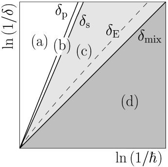
Figure 1: Schematic view of different regimes (a-d) of fidelity decay in the regime of classically chaotic (or mixing) dynamics.

Yet in the regime of non-ergodic, say integrable classical mechanics things are simpler, as we do not have to worry about the average plateau in the correlation function due to a finite ${\cal N}$ because we already have a higher average time correlation $\bar{C}\to\bar{C}_{\rm cl}\neq 0$ (18). Thus we have here only two relevant time-scales, namely $\tau_{\rm ne}$ giving initial quadratic decay (19), and the saturation time-scale $t_{*}$, due to finite size fidelity fluctuation, which depends on the properties of the initial state (power law (26) for a random initial state, versus Gaussian (31) for a coherent initial state). However in the particular special case of ‘ergodic’ perturbation $\bar{V}=0$ of regular dynamics (as mentioned above), one now clearly obtains that $\bar{C}=0$ which is equivalent of having all diagonal matrix elements vanishing, i.e. $V_{nn}=0$ [see eq. (37)]. In this case the time scale of fidelity decay $\tau_{\rm ne}$ from eq. (19) formally diverges. This in fact means that fidelity decays much slower than in generic case, now the decay being described by the first nonvanishing – i.e. fourth order term in the $\delta$-expansion.[24]

Note that our result is not contradicting any of the known facts of the quantum-classical correspondence. For example, a growth of quantum dynamical entropies [27] persists only up to logarithmically short Ehrenfest time $t_{\rm E}$, which is the upper bound for the validity of the strict classical-quantum correspondence in the fidelity decay as derived in Ref.[4, 14] and within which one would always find $F^{\rm coh}_{\rm ne}(t)>F_{\rm em}(t)$ above the perturbative border $\delta>\delta_{\rm p}$, whereas our theory reveals new nontrivial quantum phenomena with a semiclassical prediction (but not correspondence!) much beyond that time. On one hand, if we let $\hbar\to 0$ first, and then $\delta\to 0$, we recover a result supported by a classical intuition, namely that the regular (non-ergodic) dynamics is more stable than the chaotic (ergodic and mixing) dynamics. On the other hand, if we let $\delta\to 0$ first, and only after that $\hbar\to 0$, we find somewhat counterintuitive results saying that chaotic (mixing) dynamics is more stable than the regular one.

3 Purity fidelity

In this section we propose another characteristic which describes the quality of Loschmidt echoes, in particular for systems composed of two parts corresponding to different degrees of freedom, for example the central system and the environment.

We consider a system with a product Hilbert space ${\cal H}={\cal H}_{1}\otimes{\cal H}_{2}$, where ${\cal H}_{1,2}$ are factor Hilbert spaces of the two subsystems. We are again studying an echo experiment, now with the the initial state beeing a product state

$$|\psi(0)\rangle=|\psi_{1}\rangle\otimes|\psi_{2}\rangle,$$ (45)

yielding a, generally entangled, final state

$$|\psi(t)\rangle=M_{\delta}(t)|\psi(0)\rangle.$$ (46)

The entanglement produced by imperfect quantum echo can be most directly characterized by the reduced density matrix

$$\rho_{1}(t)=\,{\rm tr}\,_{2}|\psi(t)\rangle\langle\psi(t)|=\,{\rm tr}\,_{2}\left(M_{\delta}(t)|\psi(0)\rangle\langle\psi(0)|M^{\dagger}_{\delta}(t)\right)$$ (47)

obtained by tracing out the second subsytem ${\cal H}_{2}$. Now one can say that $|\psi(t)\rangle$ is disentangled iff the density matrix $\rho_{1}(t)$ is pure, and entanglement can be characterized by purity; specifically for the echo situation we call this quantity purity fidelity

$$F_{\rm P}(t)=\,{\rm tr}\,_{1}[\rho_{1}(t)]^{2}.$$ (48)

Note that purity fidelity is in some sense a weaker quantity than fidelity: in order for fidelity to be high, purity fidelity must also be high, but not vice versa. High purity fidelity only requires the state to return to the factorized form, which is a much weaker condition than complete recurrence as required by high fidelity.

Now we apply our perturbative expansion of the echo operator (8) to the expression for purity fidelity (48). Keeping only terms up to second order in the perturbation strength $\delta$ we obtain a linear response formula for purity fidelity,

$$F_{\rm P}(t) = 1-2\delta^{2}\hbar^{-2}\left\{C_{\rm int}(t)-D_{\rm int}(t)\right\}+\cdots,$$ (49)

$$D_{\rm int}(t) := \sum_{\nu\neq 1}|\langle 1,\nu|\Sigma(t)|1,1\rangle|^{2}+\sum_{i\neq 1}{|\langle i,1|\Sigma(t)|1,1\rangle|^{2}},$$

which is analogous to a simpler formula (11) for fidelity. We have used an explicit notation of a complete basis of a product Hilbert space as $|i,\nu\rangle=|i\rangle\otimes|\nu\rangle$ where latin indeces label states in the first and greek indeces states in the second subspace. There is a general relation between fidelity and purity fidelity which can be formulated in terms of a rigorous mathematical inequality[28]

$$F_{\rm P}(t)\geq F^{2}(t).$$ (50)

The formal similarity of linear response formulae (11) and (49) results in similar physical behaviour of fidelity and purity fidelity, in both qualitatively different cases of dynamics, ergodic and mixing — chaotic, and regular. For example, in the regime of ergodic and mixing dynamics we can use the result that fidelity is after a while, due to ergodicity, independent of the initial state, hence we can write for the echo operator in the weak limit sense

$$M_{\delta}(t)\to\exp(-t/\tau_{\rm em})\mathbbm{1}.$$ (51)

Plugging this expression into formula (47) and the obtained result into formula (48) we finally obtain a simple expression compatible with the upper bound of the inequality (50)

$$F_{\rm P}(t)=\exp(-4t/\tau_{\rm em}).$$ (52)

In this case the relative weight of the correction term $D_{\rm int}$ in the linear response formula (49) vanishes in proportion to $C_{\rm int}$ in the semiclassical limit $\hbar\to 0$, ${\cal N}\to\infty$. Again, the same consideration of time and perturbation scales applies for finite ${\cal N}$ as discussed above for the case of fidelity.

In the non-mixing or classically regular case, the situation is more complicated as purity fidelity depends on the structure of initial state $|\psi\rangle$. The only thing we can state generally in this case is the quadratic decay in the linear response regime, i.e. as long as $1-F_{\rm P}(t)$ is small we have

$$F_{\rm P}(t)=1-\frac{2\delta^{2}}{\hbar^{2}}(\bar{C}-\bar{D})t^{2}+{\cal O}(t^{3}).$$ (53)

Since in this case time-averaged correlation functions are non-vanishing, the integrated ones grow as $\propto t^{2}$, so we have written $C_{\rm int}(t)=\bar{C}t^{2}$, $D_{\rm int}(t)=\bar{D}t^{2}$. It is interesting to discuss the two extreme cases of intial states: (i) In the case of coherent initial states (Gaussian wave packets) we have shown [11] that the term $\bar{D}$ cancels the term $\bar{C}$ in the leading semiclassical order, so $\bar{C}-\bar{D}\propto\hbar^{2}$, whereas $\bar{C}\propto\hbar$. This means that purity fidelity for coherent initial states decays with an $\hbar$ independent time scale which is by a factor proportional to $\hbar^{-1/2}$ longer than the time scale of fidelity decay. (ii) On the other hand, in the case of initial random states one can show that the term $\bar{D}$ is negligible compared to $\bar{C}$ in the semiclassical limit, so both, fidelity, and purtity fidelity decay with the same rate, simliarly as in the case of chaotic dynamics.

There is an important special case of potential practical interest, if the perturbation is such that the unperturbed composite system is decoupled, i.e. $U_{\delta=0}=U_{1}\otimes U_{2}$. Then the unperturbed (e.g. forward) evolution does not change the purity, so the purity fidelity (purity of echo dynamics) is the same as purity (or linear entropy) of uni-directed time-evolution alone. Again, our linear response formalism predicts faster increase of linear entropy (decay of purity) for regular or weakly chaotic systems than for strongly chaotic systems.[12] This result has been independently reproduced in Ref.[29].

In next section we outline some of our numerical results which confirm the theory of the last two sections.

4 Numerical experiments

We shall consider two numerical toy models by which we may demonstrate and verify the theoretical results of previous sections.

First we choose Haake’s quantized kicked top [30] since this model served as a model example for many related studies, see e.g. Refs.[31, 13, 27, 32, 33, 34, 35]. The unitary propagator of the kicked top reads

$$U=U(\alpha,\gamma)=\exp{(-i\gamma J_{\rm y})}\exp{(-i\alpha J_{\rm z}^{2}/2J)},$$ (54)

where $J_{k}$ ($k={\rm x,y,z}$) are quantum angular momentum operators obeying $[J_{k},J_{l}]=i\epsilon_{klr}J_{r}$. The (half)integer $J$ determines the size of the Hilbert space $2J+1$ and the value of the effective Planck constant $\hbar=1/J$. The perturbation is defined by varying the parameter $\alpha$, $U_{\delta}=U(\alpha+\delta,\gamma)$, so $V$ reads

$$V=\frac{1}{2}\left(\frac{J_{\rm z}}{J}\right)^{2}.$$ (55)

The classical limit is obtained by letting $J=1/\hbar\to\infty$ and writing the classical angular momentum in terms of a unit vector on a sphere ${\bm{r}}=(x,y,z)={\bm{J}}/J$. The Heisenberg equation for the SU(2) operators ${\bm{J}}$, ${\bm{J}}^{\prime}=U^{\dagger}{\bm{J}}U$, reduces to the classical area preserving map of a sphere

$$x^{\prime} = \cos{\gamma}(x\cos{\alpha z}-y\sin{\alpha z})+z\sin{\gamma}$$

$$y^{\prime} = y\cos{\alpha z}+x\sin{\alpha z}$$

$$z^{\prime} = z\cos{\gamma}+\sin{\gamma}(y\sin{\alpha z}-x\cos{\alpha z}).$$ (56)

Note that in the classical limit the perturbation generator is

$$v({\bm{r}})=\frac{z^{2}}{2}.$$ (57)

For $\alpha=0$ the system is integrable, while with increasing $\alpha$ there is a transition to chaotic motion. The second parameter $\gamma$ is usually set to $\pi/2$, however in our numerical simulation we will use two different values exhibiting qualitatively different correlation decay (for large $\alpha$): the ’standard’ case $\alpha=30,\gamma=\pi/2$ where $C_{\rm cl}(t)$ decays in oscillatory way and the case $\alpha=30,\gamma=\pi/6$ where $C_{\rm cl}(t)$ decays monotonically (see fig. 4).

In the case of $\gamma=\pi/2$ we have two discrete symmetries. The evolution $U$ commutes with $R_{\rm x}$ and $R_{\rm y}$, the rotations of $\pi$ around the ${\rm x}$ and ${\rm y}$ axes, respectively. The Hilbert space is therefore reducible into three invariant subspaces (using notation of Peres’s book [2] with the basis $|m\rangle$ of eigenstates of $J_{\rm z}$ and assuming $J$ to be an even integer): EE of dimension $J/2+1$ with the basis states $|0\rangle$ and $\{|2m\rangle+|-2m\rangle\}/\sqrt{2}$; OO of dimension $J/2$ with the basis $\{|2m-1\rangle-|-(2m-1)\rangle\}/\sqrt{2}$; OE of dimension $J$ with the basis $\{|2m\rangle-|-2m\rangle\}/\sqrt{2}$ and $\{|2m-1\rangle+|-(2m-1)\rangle\}/\sqrt{2}$ with $m=1,\ldots,J/2$ in all three cases. For $\gamma\neq\pi/2$ the spaces OO and EE coalesce as $R_{\rm y}$ is the only discrete symmetry left. In numerical experiments we always choose the OE subspace so that the dimension of the Hilbert space is ${\cal N}=J$.

We will compute the fidelity of two different types of initial states: (1) random initial state with components $c_{m}=\langle m|\psi\rangle$ being independent Gaussian pseudo-random numbers, and (2) pure minimal wavepacket initial state, namely SU(2) coherent state $|\psi\rangle=|\vartheta,\varphi\rangle$ centered at the point ${\bm{n}}=(\sin{\vartheta}\cos{\varphi},\sin{\vartheta}\sin{\varphi},\cos{\vartheta})$ on a unit sphere

$$|\vartheta,\varphi\rangle=\sum_{m=-J}^{J}{\left({2J\atop J+m}\right)^{1/2}\cos{(\vartheta/2)}^{J+m}\sin{(\vartheta/2)}^{J-m}e^{-im\varphi}|m\rangle}.$$ (58)

As a second model we choose a Jaynes-Cummings (JC) Hamiltonian, a popular model in the realm of quantum optics. JC model is an autonoumous (time-independent) system of an harmonic oscillator interacting with a rotor, e.g. one mode of electromagnetic field, and a spin, say of an atom. Suppose the oscillator is described by standard anihilation/creation operators $a,a^{\dagger}$, and the spin of (half)integer value $J$ by SU(2) variables $J_{\pm},J_{\rm z}$. Then the JC Hamiltonian reads

$$H=\hbar\omega a^{\dagger}a+\hbar\epsilon J_{\rm z}+\frac{\hbar}{\sqrt{2J}}\left(G(aJ_{+}+a^{\dagger}J_{-})+G^{\prime}(aJ_{-}+a^{\dagger}J_{+})\right).$$ (59)

Here the last (counter rotating) term has been included to allow for chaotic motion [36] Contrary to the kicked top model and the framework of previous theoretical discussion, time $t$ is here a continuous variable. There is, however, a natural limiting procedure in order to obtain continuous time versions of results of sections 2 and 3 by replacing all the sums like $\sum_{t^{\prime}=0}^{t-1}$ by integrals $\int_{0}^{t}dt^{\prime}$. A convenient scaling towards the classical limit $J\to\infty$, $\hbar\to 0$, is obtained by fixing classical angular momentum $\hbar J=1$, hence $\hbar=1/J$. We perturb JC model by detuning, i.e. slightly changing the magnetic field parameter $\epsilon$, so the generator of perturbation reads $V=\hbar J_{\rm z}$. As an initial state we here choose only the coherent state, namely a direct product of oscillator coherent state with complex parameter $\alpha$, and SU(2) coherent state with another complex parameter $\tau=e^{i\varphi}\tan(\vartheta/2)$:

$$|\psi\rangle=e^{\alpha a^{\dagger}-\alpha^{*}a}|0\rangle_{2}\otimes(1+|\tau|^{2})^{-J}e^{\tau J_{-}}|J,J\rangle_{1}.$$ (60)

The classical JC Hamiltonian is integrable if either $G=0$ or $G^{\prime}=0$, whereas it can display all the variety of KAM regimes as both parameters $G$, $G^{\prime}$ are increased and reaching practical ergodicity for sufficiently large $G,G^{\prime}$. We study numerically two different sets of parameters: In both we choose $\omega=\epsilon=0.3$, and (i) $G=1,G^{\prime}=0$ corresponding to classically regular motion, and (ii) $G=G^{\prime}=1$ corresponding to classically almost fully chaotic motion. In both cases we choose the same initial coherent state with parameters $\alpha=1.15,\tau=0.29+{\rm i}0.46$ and set angular momentum $J=4$. We first choose a small perturbation parameter $\delta=0.005$. Numerical results of time correlation functions and fidelity decay in such a linear response regime are shown in figs. 2,3.

Figure 2: Integrated quantum correlation function of the perturbation in the JC model, divided by time $t$. Solid curve corresponds to classically chaotic case (see text) and is approaching a constant plateau (dashed), whereas dotted curve corresponds to integrable case (see text) following linear growth (dashed).

Figure 3: Fidelity decay of the coherent initial state in JC model for regular and almost fully chaotic dynamics (see text). Dotted and full curves correspond to numerically exact evaluations of fidelity, whereas circles and squares reproduce a precise evaluation of the linear response formula (9) in terms of quantum correlation functions (of fig. 2). Dashed curves are best fitting linear and quadratic decays.

In order to reach beyond the linear response regime and go deeper into the semiclassical regime we use the kicked top model. There we may hope to exploit the behaviour of classical correlation functions in order to predict quantum fidelity decay. First, we turn to the regime of completely chaotic classical dynamics.

Figure 4: Classical correlation function $C_{\rm cl}(t)$ for kicked top with $\alpha=30$, and $\gamma=\pi/6$ (top, full curve) and $\gamma=\pi/2$ (bottom, broken curve). Finite time integrated correlation function is shown in the inset, converging to $\sigma_{\rm cl}=0.00385$ and $0.0515$, for $\gamma=\pi/2$ and $\pi/6$, respectively. Averaging over $10^{5}$ random initial conditions on a sphere is performed.

The classical correlation functions calculated by using the classical map (56) are shown in fig. 4. For $\alpha=30,\gamma=\pi/2$ the correlation function is oscillating with an exponential envelope hence the transport coefficient $\sigma_{\rm cl}=0.00385$ is quite small. For $\alpha=30,\gamma=\pi/6$ the correlation decay is monotonic and exponential with $\sigma_{\rm cl}=0.0515$. The decay of quantum fidelity (17) can now be obtained by using the classical limit $\sigma\to\sigma_{\rm cl}$:

$$F_{\rm em}(t)=\exp{(-2\delta^{2}J^{2}\sigma_{\rm cl}t)}.$$ (61)

This formula has been compared with the exact numerical calculation of fidelity averaging over a set of random initial states. We stress that we found no observable difference for sufficiently large $J$ when we have instead chosen a fixed coherent initial state, however this calculation is not shown in the figures. As the finite size fidelity fluctuation level $F_{\rm ta}$ decreases with increasing Hilbert space dimension, we chose large $J=4000$ in order to be able to check exponential decay (61) over as many orders of magnitude as possible.

Figure 5: Quantum fidelity for a kicked top with parameters $\alpha=30$, $J=4000$ and full trace average. Top figure is for $\gamma=\pi/2$ and for $\delta=5\cdot 10^{-4},1\cdot 10^{-3},3\cdot 10^{-3}$ (solid, dashed, dotted curves, respectively) Bottom figure is for $\gamma=\pi/6$ and $\delta=1\cdot 10^{-4},2\cdot 10^{-4},3\cdot 10^{-4}$, (solid, dashed, dotted curves, respectively). Chain line in both cases gives the theory (61) with classically computed $\sigma_{\rm cl}$. Note that the largest $\delta=3\cdot 10^{-3}$ case in the top figure (dotted curve) corresponds to $\tau\approx 2$, so it is already over the upper border of the regime (c, subsect. 2.3) $\delta>\delta_{\rm mix}$ but the agreement with the theory (61) is still quite good, appart from oscillations. This is due to the oscillatory nature of time-correlations making the factorization assumption (16) justified (on average) even for much smaller time $t$ as required.

The results are shown in fig. 5. The smallest and the largest $\delta$ shown, roughly correspond to borders $\delta_{\rm s}$ and $\delta_{\rm mix}$, respectively. As we can see, the agreement with an exponential decay is excellent, at least over four decades in the fidelity $F(t)$. Note that for $\gamma=\pi/2$ and the largest $\delta=3\cdot 10^{-3}$ the time-scale of the decay of fidelity is comparable to the classical time-scale $t_{\rm mix}$ so the factorization assumption (16) is strictly no longer applicable. However, due to oscillatory correlation decay, overall agreement with the theory (61) is still rather good, but the oscillations of the correlation decay are reflected by oscillations of the fidelity decay (around the theoretical exponential curve). Of course one does not need such a large $J$ in order to have an exponential decay, but for smaller $J$ the fluctuation level $F_{\rm ta}$ will be higher so the exponential decay (61) will persist for correspondingly smaller time.

Figure 6: Finite time quantum correlation sum $\sigma(t)=\sum_{t^{\prime},t^{\prime\prime}=0}^{t-1}{C(t^{\prime},t^{\prime\prime})/2t}$ (solid curves) and the corresponding classical sum $\sigma_{\rm cl}(t)=\sum_{t^{\prime},t^{\prime\prime}=0}^{t-1}{C_{\rm cl}(t^{\prime},t^{\prime\prime})}/2t$ (dashed curves saturating at $\sigma_{\rm cl}$ and ending at $t\sim 1000$) for $\alpha=30,J=1500$. Upper curves are for $\gamma=\pi/6$ while lower curves are for $\gamma=\pi/2$. Chain lines are best fitting asymptotic linear functions corresponding to $\bar{C}t$, $0.0077t/J$ for $\gamma=\pi/2$ and $0.103t/J$ for $\gamma=\pi/6$.

Then we focus on the so-called perturbative regime $\delta<\delta_{\rm p}$ where the fidelity decay will be dictated by a finite size correlation average (38), so according to eq. (41)

$$F_{\rm pert}(t)=\exp{(-4\delta^{2}J\sigma_{\rm cl}t^{2})}.$$ (62)

We numerically computed $\bar{C}$ (18) for $J=1500$, $\alpha=30$ in order to show that it is given by the theoretical value (38). The quantum correlation function has been computed $C(t^{\prime},t^{\prime\prime})=\langle\tilde{V}_{t^{\prime}}\tilde{V}_{t^{\prime\prime}}\rangle$ by means of a traceless perturbation $\tilde{V}=\frac{1}{2}(J_{z}/J)^{2}-\frac{1}{12}[(2J+1)(J+1)/J^{2}]\mathbbm{1}$. In fig. 6 we show a finite time correlation sum $\sigma(t)=\frac{1}{2t}\sum_{t^{\prime},t^{\prime\prime}=0}^{t-1}C(t^{\prime},t^{\prime\prime})$ which exhibits a crossover, at the Heisenberg time $t_{\rm p}=J/2$, from the plateau given by $\sigma_{\rm cl}$ to a linear increase $\bar{C}t$ due to finite size correlation average (38) $\bar{C}=4\sigma_{\rm cl}/J$.

Figure 7: Quantum fidelity in the perturbative regime $\delta<\delta_{\rm p}$ for $\alpha=30$, $J=1500$, and $\gamma=\pi/2$ and $\pi/6$, calculated as a full trace Hilbert space average as a function of the scaled variable $J(\delta t)^{2}$. For $\gamma=\pi/2$ data for $\delta=1\cdot 10^{-6}$ (solid curve) and $5\cdot 10^{-6}$ (dotted curve) are shown. For $\gamma=\pi/6$, $\delta=3\cdot 10^{-7}$ (solid) and $1\cdot 10^{-6}$ (dotted) are shown. Note that for both $\gamma$ the curves for both $\delta$ practically overlap. The chain curves are theoretical predictions (62) with classically computed $\sigma_{\rm cl}$.

The excellent agreement between prediction (62) and full numerical calculation of fidelity is shown in fig. 7. In view of our findings this so-called [13] perturbative regime can be understood as a simple consequence of a finite Hilbert space dimension. For times larger than the Heisenberg time $t_{\rm p}$ every quantum system behaves effectively as an integrable one, i.e. with a finite time average correlation plateau.

Next, we turn to the regime of nonergodic, say regular classical dynamics of the kicked top, which is realized for small value of $\alpha$. If the classical phase space has a mixed (KAM) structure, the non-mixing regime of fidelity decay may be obtained by choosing a localized initial state (e.g. coherent state) located in a regular part of the phase space. Such a situation may easily lead to the opposite conclusion (as compared to generic situation) for an insufficiently large dimension ${\cal N}$. As discussed in subsect.2.3, the fidelity fluctuation plateau is determined by the number of constituent propagator eigenstates $|\phi_{n}\rangle$ which are effectively needed to expand the initial state. For a coherent state sitting inside a (not too large) regular (KAM) island this number can be fairly small for numerically realizable Hilbert space dimensions, thus prohibiting any significant fidelity decay as observed in Ref.[3] We would still see the initial quadratic decay in the linear response regime but we would not be able to verify higher orders in the long-time expansion of fidelity. In order to produce a situation numerically as clean as possible, we choose a small value of parameter $\alpha=0.1$, such that the classical dynamics is almost integrable and the majority of phase space corresponds to regular motion so that the number of constituent eigenstates for coherent states is as large as possible (on average).

Here we focus on the case $\gamma=\pi/2$. For small $\alpha$, the quantum and classical evolution is a (slightly perturbed) rotation around ${\rm y}$ axis and the time averaged perturbation can be computed analytically (to leading order in $\alpha$) as

$$\bar{V}=\frac{1}{4J^{2}}(J_{\rm z}^{2}+J_{\rm x}^{2})=\frac{1}{4}\left(1-(J_{\rm y}/J)^{2}\right),\qquad\bar{v}=\frac{1}{4}(1-y^{2}).$$ (63)

We will now use these approximate analytical results for $\alpha\to 0$ to compare with numerics for $\alpha=0.1$. Note that our leading order analytical approximations could easily be systematically improved using a classical perturbation theory (treating $\alpha$ as a perturbing parameter). Since the agreement, as shown below, is almost perfect in all cases, we see no need for refinement at this level.

First consider a random initial state. Starting from expression (21), $F(t)=|\langle\exp{(it\bar{V}\delta/\hbar)}\rangle|^{2}$, write the fidelity as a sum over all eigenvalues of $J_{\rm y}^{2}$, namely $(2m-1)^{2}$, for $m=1,\ldots,J/2$ (in OE subspace),

$$F(t)=\left|\frac{2}{J}\sum_{m=1}^{J/2}{\exp{(i\delta t(2m-1)^{2}/4J)}}\right|^{2}.$$ (64)

For large $J$ we can replace the sum with an integral and get

$$F(t)=\frac{\pi}{\delta Jt}\left|{\rm erfi}(\frac{1}{2}e^{i\pi/4}\sqrt{\delta Jt})\right|^{2},$$ (65)

Figure 8: Fidelity in the near-integrable regime for $\alpha=0.1$, $\gamma=\pi/2$, $\delta=0.01$, $J=100$, and $\rho=\mathbbm{1}/J$, in the OE subspace. Solid curve gives the result of a numerical simulation. Isolated dots denote differences between numerical calculation and the analytic formula (65) for $\alpha\to 0$ $|F_{\rm num.}(t)-F_{\rm anali.}(t)|$. The dotted line gives the predicted asymptotic decay $\propto t^{-1}$, and the dashed/chain curves are the predicted fidelity decays at small times, namely the second order expansion $F(t)=1-(Jt\delta)^{2}/180$, and the ’improved’ Gaussian result $F(t)=\exp(-(Jt\delta)^{2}/180)$.

where ${\rm erfi}(z)=\frac{2}{i\sqrt{\pi}}\int_{0}^{iz}{e^{-t^{2}}dt}$ is a complex error function with an asymptotic limit $\lim_{x\to\infty}{|{\rm erfi}(\frac{1}{2}e^{i\pi/4}\sqrt{x})|}=1$ to which it approaches by oscillating around $1$. We thus have an analytic expression for the fidelity (65) in the case of an uniform average over the Hilbert space or, equivalently, for a random initial state. Its asymptotic decay is $t^{-1}$ which agrees with the general semiclassical asymptotics (26). We expect initial quadratic decay (19) for small times $t<\tau_{\rm ne}$. The decay rate $\tau_{\rm ne}$ is determined by the time averaged correlation $\bar{C}$ (18) which can be calculated explicitly in the limit $\alpha\to 0$ where the classical correlation function $C_{\rm cl}(t)$ alternates for even/odd times as $C_{\rm cl}(2t)=\langle\tilde{z}^{2}(0)\tilde{z}^{2}(2t)\rangle/4=-1/90$, $C_{\rm cl}(2t+1)=\langle\tilde{z}^{2}(0)\tilde{z}^{2}(2t+1)\rangle/4=1/45$, giving

$$\bar{C}_{\rm cl}|_{\alpha=0}=\frac{1}{2}\left(-\frac{1}{90}+\frac{1}{45}\right)=\frac{1}{180}.$$ (66)

Fidelity is expected to decay as (19) with $\tau_{\rm ne}=\sqrt{180}/(J\delta)$, for short times, $t<\tau_{\rm ne}$. The short-time formula (19) and the full analytic expression (65) are compared with the numerical simulation in fig. 8. The agreement is very good and, surprisingly enough, the Gaussian approximation $F(t)=\exp(-(t/\tau_{\rm ne})^{2})$ for small times is observed to be valid considerably beyond the second order expansion (19). Quite interesting is the regime where the decay time $\tau_{\rm ne}=\sqrt{180}/(J\delta)$ for a “regular” dynamics with a random initial state will be smaller than the decay time $\tau_{\rm em}=1/(\delta^{2}J^{2}\sigma_{\rm cl})$ (61) for a “chaotic” dynamics. This will happen for $\delta<1/(J\sigma_{\rm cl}\sqrt{180})$. This border has the same scaling with $J$ as $\delta_{\rm mix}$ (43).

Figure 9: Fidelity for $\gamma=\pi/2$, $\delta=0.025$ and $J=100$ on the OE subspace. The dashed curve is a simulation for $\alpha=30$ (mixing regime, full trace average). The pluses are for a pure coherent initial state (see text for details) at $\alpha=0.1$ (non-mixing regime). The chain and solid curves are, respectively, the theoretical exponential (61) and Gaussian (69) decays.

Second we consider an SU(2) coherent initial state (58). We could perform an exact analytical calculation for the fidelity decay in this particular case. Rather than performing this calculation, we will illustrate the usefulness of a semiclassical formula for $F_{\rm ne}^{\rm coh}(t)$ (31). This is a more general approach, as an explicit analytical calculation is usually not possible. Let us denote by $\tilde{\vartheta},\tilde{\varphi}$ the spherical angular coordinates measured with respect to the y-axis. Then $(I=\cos\tilde{\vartheta}=y,\tilde{\varphi})$ represent canonical action-angle coordinates for the integrable case $\alpha\to 0$. Furthermore, the coherent state (58) acquires a semiclassical Gaussian form (27) in the EBK basis $|n\rangle$, $J_{\rm y}|n\rangle=n|n\rangle$, namely

$$|\langle n|\tilde{\vartheta},\tilde{\varphi}\rangle|^{2}\propto\exp{\left(-\frac{(n\hbar-\cos{\tilde{\vartheta}})^{2}}{\hbar\sin^{2}{\tilde{\vartheta}}}\right)},\quad\hbar=\frac{1}{J}.$$ (67)

The squeezing parameter $\Lambda$ reads

$$\Lambda=1/\sin^{2}{\tilde{\vartheta}}=1/(1-y^{2}).$$ (68)

In order to apply the general formula (31) we need to express the classical time average (63) in terms of a canonical action, $\bar{v}(I)=(1-I^{2})/4$, and evaluate the derivative, $|\partial\bar{v}(I)/\partial I|^{2}=\frac{1}{4}I^{2}$, giving $F^{\rm coh}_{\rm ne}(t)=\exp{(-\delta^{2}Jt^{2}I^{2}(1-I^{2})/8)}$. Rewriting this expression in terms of original spherical angles $\vartheta$ and $\varphi$ measured with respect to ${\rm z}$-axis, we obtain

$$F^{\rm coh}_{\rm ne}(t)=\exp{\left(-\frac{\delta^{2}Jt^{2}}{32}\{\sin^{2}{2\vartheta}\sin^{2}{\varphi}+\sin^{4}{\vartheta}\sin^{2}{2\varphi}\}\right)}.$$ (69)

We checked this formula by means of a numerical simulation and the result for a coherent state centered at $(\vartheta,\varphi)=\pi(1/\sqrt{3},1/\sqrt{2})$, for which $\sin^{2}{2\vartheta}\sin^{2}{\varphi}+\sin^{4}{\vartheta}\sin^{2}{2\varphi}=0.96$, is shown in fig. 9. We can see that for $t>50$ the fidelity in a non-mixing regime ($\tau_{\rm ne-coh}=23$) is lower than the fidelity in a mixing regime ($\tau_{\rm em}=42$). For larger times, $t>t^{*}$, non-mixing decay $F^{\rm coh}_{\rm ne}$ displays revivals of fidelity which are a simple manifestation of a beating phenomenon due to sligtly different frequencies of revolution of wave-packets along unperturbed and perturbed KAM tori. Note that this effect of revivals is drastically reduced in more than one dimension, $d\geq 2$, where there are typically several different incomensurate frequencies [7].

Figure 10: Purity fidelity $F_{\rm P}(t)$ (main figure) and squared fidelity $[F(t)]^{2}$ (inset) in chaotic regime (solid curves) and in integrable regime (dotted curves), for $\delta=0.1$. The dashed lines indicate the linear and quadratic approximation respectively. Note the differences in vertical scales.

Next we make numerical experiments on the decay of purity fidelity. Again we choose the JC Hamiltonian and treat the oscillator and the spin as two parts of a composite system. We first report a calculation with a strong perturbation $\delta=0.1$, that rapidly exceeds the realm of validity of linear response, in Fig. 10 where the main figure gives the purity fidelity and the inset the fidelity for comparison. For the fidelity decay (inset) we find excellent agreement with exponential decay (17) in a chaotic regime and with a faster Gaussian decay in a regular regime (31), where the decay rates are fixed as above. For purity fidelity, however, we find already at $t\approx 20$, that the decay starts to be influenced by the saturation value of $F_{\rm P}(t\to\infty)\approx 1/(2J+1)$. Therefore purity fidelity is higher for the integrable case than for the chaotic one not only at short times, as expected, but even at large times. This is relevant, because we shall next choose a weak perturbation $\delta=0.005$ to avoid this problem.

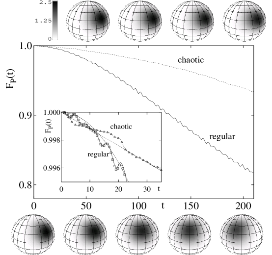
Figure 11: Echo dynamics for weak coupling: $\delta=0.005$. Square of the Wigner function for chaotic dynamics (top diagrams) and integrable dynamics as a function of time (bottom diagrams) at times corresponding to the axis. Grey code: top left. Purity fidelity is shown in the frame on the same time scale and for short times in the inset. Full curves show the complete numerics, symbols the evaluation starting from the numerical correlation functions of Fig. 2 and dashed curves the linear or quadratic approximation.

We expect and find the crossover after a fairly short time. This calculation allows comparison with theory as well as an illustration of the evolution of the square of the Wigner function, corresponding to the reduced density matrix $\rho_{1}(t)$ for the angular momentum states on the sphere using the definition of Ref.[37]. Near the top and bottom of Fig. 11 we see this evolution for the chaotic and the integrable Hamiltonian respectively. In the center of the figure we plot the purity fidelity on the same time scale as the Wigner functions in the main frame and an amplification of short times in the inset. Again, we note faster decay of purity fidelity in the case of regular dynamics as compared to chaotic dynamics. We observe detailed agreement of numerics with results obtained from the numerical values of the correlation integrals (9,49) reproducing the oscillatory structure. From the same correlation integrals we obtained the coefficients for the linear and quadratic decay, which agree well if we discard the oscillations. We see a crossing of the two curves at $t=t^{*}_{\rm P}\approx 12$ for $F_{\rm P}$. These times are larger than the Zeno time ($\approx 1$) and indicate the competition of the decay rate and the decay shape as expected for a non-small value of $\hbar=1/4$. It is important to remember that the integral over the square of the Wigner function gives the purity and therefore the fading of the picture will be indicative of the purity decay. On the other hand the movement of the center is an indication of the rapid decay of fidelity (not shown in the figure).

5 Summary and discussion

In this paper we have outlined a simple theory of stability of quantum time evolution with respect to small variation of the Hamiltonian or, more generally, of the time-evolution propagator. The central object of study is the fidelity, a cross correllation between two states originating from the same initial state but subject to two slightly different time evolutions. An alternative interpretation of the whole theoretical setup can be given in terms of quantum dynamical irreversibility in the Loschmidt echo gedanken experiment. This intepretation allows even for more general characterization of the quality of quantum echo, as given for example by purity fidelity which measures the quality with which the final state, after an echo experiment, factorizes in the direct product Hilbert space of a composite system. When one part of a composite system is interpreted as environment, then the decay of purity fidelity can be directly linked to the growth of decoherence.

The main result reported here is a simple linear response (or Kubo-like) formula (9) which relates the fidelity decay, and quite similarly also the purity fidelity decay, to the total sum (or integral) of two point time autocorrelation function of the perturbation. In the limit of infinite Hilbert space dimension we have found exponential fidelity decay on a time-scale $\tau_{\rm em}\propto(\hbar/\delta)^{2}$, for quantum ergodic and mixing systems, whereas for non-ergodic systems we have found much faster decay (in the sufficiently ‘quantum’ regime where $\delta\ll\hbar$, but note that both, $\delta$ and $\hbar$ are dimensionless parameters) on a time-scale $\tau_{\rm ne}\propto\hbar/\delta$ for random initial states or $\tau_{\rm ne-coh}\propto\hbar^{1/2}/\delta$ for coherent initial states (minimal uncertainty wavepackets) where the fidelity $F(t)$ is given by a Fourier transformation of the local density of states of the time averaged perturbation operator. A special emphasis has been given to the semiclassical theory of fidelity of small but finite values of $\hbar$, where different regimes and the corresponding time and perturbation scales are carefully discussed, and where fidelity decay may asymptotically (as $\hbar\to 0$) be evaluated in terms of classical quantities only. Interestingly, finite size fluctuations of fidelity (for very long times at a finite Hilbert space dimension) have been shown to be given by the inverse participation ratio of the eigenstates of the perturbed evolution operator in the eigenbasis of the unperturbed propagator. The surprising aspects of our relations are basically due to non-interchangability of the limits $\delta\to 0$ and $\hbar\to 0$ as the relevant decay time-scales are only functions of the ratio $\delta/\hbar$. Therefore a different and intuitively expected behaviour, namely faster fidelity decay for mixing than regular dynamics, is obtained in the ‘classical’ regime where $\hbar\ll\delta$ (or making the limit $\hbar\to 0$ prior to $\delta\to 0$). We should note that a similar, reassuring result has been found by applying our formalism to inspect the analogous classical fidelity[7, 17, 18] for the unitary Perron-Frobenius evolution of volume (area) preserving maps [7]: there the classical fidelity for regular dynamics has been found to decay on a time-scale $\propto\delta^{-1}$, i.e. the same as for quantum fidelity decay of regular dynamics, whereas for a chaotic dynamics, the fidelity decay is governed by a maximal Lyapunov exponent $\lambda$ on a short time-scale $\propto\ln(1/\delta)/\lambda$.

Our findings may have some important implication in the understanding of the stability of quantum computation [9] where different regimes and time-scales [38] should perhaps be explained in terms of intrinsic dynamics of a particular quantum algorithm. On the other hand, our results may also shed new light on the relation between decoherence and dynamics [6]. In particular, due to the quite special role of coherent initial states on the short Ehrenfest time-scale one may expect the results to be quite different for a random initial state and/or for longer time-scales (see [39]).

References

- [1] G. Casati, B. V. Chirikov, I. Guarneri and D. L. Shepelyansky, Phys. Rev. Lett. 56 (1986), 2437.
- [2] A. Peres, Quantum Theory: Concepts and Methods (Kluwer, Dordrecht, 1995).
- [3] A. Peres, Phys. Rev. A 30 (1984), 1610; see also the book [2].
- [4] R. A. Jalabert and H. M. Pastawski, Phys. Rev. Lett. 86 (2001), 2490.
- [5] G. P. Berman and G. M. Zaslavsky, Physica A 91 (1978), 450.
- [6] W. H. Zurek and J. P. Paz, Physica 83D (1995), 300.
- [7] T. Prosen and M. Žnidarič, J. Phys. A: Math. Gen 35 (2002), 1455.
- [8] T. Prosen, Phys. Rev. E 65 (2002), 036208.
- [9] T. Prosen and M. Žnidarič, J. Phys. A: Math. Gen. 34 (2001), L681.
- [10] T. Prosen and T. H. Seligman, J. Phys. A: Math. Gen. 35 (2002), 4707.
- [11] T. Prosen, T. H. Seligman and M. Žnidarič, Phys. Rev. A (2003) in press, quant-ph/0204043.
- [12] M. Žnidarič and T. Prosen, J. Phys. A: Math. Gen. 36 (2003), 2463.
- [13] Ph. Jacquod, P. G. Silvestrov, C. W. J. Beenakker, Phys. Rev. E 64 (2001), 055203.
- [14] F. M. Cucchietti, H. M. Pastawski and D. A. Wisniacki, Phys. Rev. E 65 (2002), 045206(R).
- [15] B. Eckhardt, J. Phys. A: Math. Gen 36 (2003), 371.
- [16] S. Tomsovic and N. Cerruti, Phys. Rev. Lett. 88 (2002), 054103.
- [17] G. Benenti and G. Casati, Phys. Rev. E 66 (2002), 066205.
- [18] G. Benenti, G. Casati and G. Veble, preprint, nlin.CD/0208003.
- [19] F. M. Cucchietti et al. Phys. Rev. E 65 (2002), 046209; D. A. Wisniacki et al. Phys. Rev. E 65 (2002), 055206; D. A. Wisniacki and D. Cohen, Phys. Rev. E 66 (2002), 046209; J. Emerson et al, Phys. Rev. Lett. 89 (2002), 284102; G. P .Berman et al, Phys. Rev. E 66 (2002) 056206; W. G. Wang and Baowen Li, Phys. Rev. E 66 (2002), 056208; T. Kottos and D. Cohen, Europhys. Lett. 61 (2003), 431; D. A. Wisniacki, Phys. Rev. E 67 (2003), 016205; P. G. Silvestrov, J. Tworzydlo and C. W. J. Beenakker, Phys. Rev. E. 67 (2003), 025204; M. F. Andersen, A. Kaplan, N. Davidson, preprint, quant-ph/0208052.
- [20] H. M. Pastawski, P. R. Levstein and G. Usaj, Phys. Rev. Lett.75 (1995), 4310; P. R. Levstein, G. Usaj and H. M. Pastawski, J. Chem. Phys. 108 (1998), 2718.
- [21] M. A. Nielsen and I. L. Chuang, Quantum computation and quantum information (Cambridge University Press, 2001).
- [22] see e.g. H. Narnhofer and W. Thirring, J. Stat. Phys. 57 (1989), 811, or G. Jona-Lasinio and C. Presilla, Phys. Rev. Lett. 77 (1996), 4322.
- [23] A. Peres, Phys. Rev. Lett. 53 (1984), 1711.
- [24] T. Prosen and M. Žnidarič, preprint, to be submitted to J. Phys. A (2003).
- [25] M. Feingold and A. Peres, Phys. Rev. A 34 (1986), 591; M. Feingold, D. M. Leitner and O. Piro, Phys. Rev. A 39 (1989), 6507; T. Prosen and M. Robnik, J. Phys. A: Math. Gen. 26 (1993), L319; T. Prosen, Ann. Phys. (NY) 235 (1994), 115.
- [26] F. Haake, Quantum signatures of chaos (Springer, Berlin, 1991).
- [27] R. Alicki, D. Makowiec and W. Miklaszewski, Phys. Rev. Lett. 77 (1996), 838.
- [28] T. Prosen, T. H. Seligman and M. Žnidarič, preprint, submitted to Phys. Rev. A (2003).
- [29] A. Tanaka, H. Fujisaki and T. Miyadera T, Phys. Rev. E 66 (2002), 045201.
- [30] F. Haake, M. Kuś and R. Schar, Z. Phys. B 65 (1987), 381; see also the book [26]
- [31] R. Shack, M. G. D’Ariano and C. M. Caves, Phys. Rev. E 50 (1994), 972.
- [32] R. F. Fox and T. C. Elston, Phys. Rev. E 50 (1994), 2553.
- [33] G. Casati, B. V. Chirikov and O. V. Zhirov, Phys. Rev. E 55 (1997), 7757.
- [34] J. K. Breslin and G. J. Milburn, Phys. Rev. A 59 (1999), 1781.
- [35] F. Haake, J. Mod. Optic. 47 (2000), 2883.
- [36] K. Furuya, M. C. Nemes and G. Q. Pellegrino, Phys. Rev. Lett. 80 (1998), 5524.
- [37] G. S. Agarwal, Phys. Rev. A 24 (1981), 2889.
- [38] P. H. Song and D. L. Shepelyansky, Phys. Rev. Lett. 86 (2001), 2162; B. Georgeot and D. L. Shepelyansky, Phys. Rev. Lett. 86 (2001), 5393.
- [39] T. Gorin and T. H. Seligman, J. Opt. B 4 (2002), 386; Phys. Lett. A 309, 61 (2003).