Schrödinger Proof in Minplus complex Analysis

Abstract.

We are presenting an internal trajectory model for a quantum particle in the Schrödinger non-relativistic approximation. This model is based on two new mathematical concepts: a complex analytical mechanics in Minplus complex analysis and a periodical non random process which gives a complex Îto formula.

This model naturally generates a concept of spin or isospin and the Heisenberg inequalities, and leads to the Schrödinger equation using a generalization of the least action principle adapted to the trajectories of this type.

1. Introduction

We are presenting a complex process to model a quantum particle in the Schrödinger non-relativistic approximation. This model naturally generates an intrinsic angular momentum and leads to the Schrödinger equation using a generalization of the least action principle.

The model is based on two new mathematical concepts that we have brought up in previous papers: a complex analytical mechanics [7],[9] and a periodical deterministic process [8].

The purpose of this paper is to develop this new model and to demonstrate some properties. We attempt to address the following questions: how does an intrinsic angular momentum emerge from the six periodical complex processes (theorem 2.7)? How can we find the Heisenberg inequalities (theorem 2.8)? the non commutation relations (theorem 2.9)? On what principle can the Schrödinger equation be demonstrated (theorems 3.4 and 3.5)? How can we find the trajectories of de Broglie and Bohm (theorem 3.6)?

2. The model of trajectory

In any orthonomal reference system R, let be U_R the set of 8 vectors $\left\{e_{1},e_{2},e_{3}\right\}$ where e${}_{i}=\pm 1$, corresponding to the eight vertices of a cube. We then consider the set S of the circular permutations of the 6 vertices of this cube to correspond to a sequence of adjacent vertices. We verify that S corresponds to the following eight permutations:

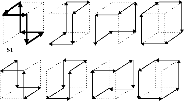
Figure 1. The eight permutations.

To each of these permutations $s\in S$, we associate the set $U_{R}^{s}$ of these vertices. This gives $s^{6}u^{j}=u^{j}$ for any $u^{j}\in U_{R}^{s}$ .

Remark 2.1.

Each of these permutations corresponds to the rotation of the cube on a diagonal. Therefore, it will be necessary to choose one of these permutations in the case of the Schrödinger equation. In the case of the Pauli equation, the frame R will no longer be fixed but will be oriented along an axis (that of the spin or isospin) which will change with time under the effect of a magnetic field.

Definition 2.2.

For any time step $\varepsilon>0$ and for any permutation $s\in S$, we define the 6 discrete processes $Z_{\varepsilon}^{j}(t)$ at time $t=n\varepsilon,$ with $n=6q+r$ ($n,q,r$ integers and $0\leq r\leq 5$), by:

(1) $$Z_{\epsilon}^{j}(\left(n+1\right)\epsilon)=Z_{\epsilon}^{j}(n\epsilon)+\mathcal{V}(6(q+1)\epsilon)\epsilon+\gamma(s^{n+1}u^{j}-s^{n}u^{j})$$

(2) $$Z_{\epsilon}^{j}(0)=Z_{0},\qquad u^{j}\in U_{R}^{s}$$

where $\gamma=$ $(1+i)\sqrt{\frac{3\hslash\varepsilon}{8m}}$ and where $\mathcal{V}(t)$ corresponds to a continuously differentiable complex function, where $\hslash$ is the Planck constant and m is the mass of the particle, and where $Z_{0}$ is a given vector of $\mathcal{C}^{3}$.

Remark 2.3.

The 6 processes $Z_{\varepsilon}^{j}(t)$ look like stochastic processes of Nelson [14],[15], but there are very different because there are deterministic. In $\left[6\right]$ p.117, Feynman and Hibbs show that the ”important paths” of quantum mechanics, although continuous, are very irregular and nowhere differentiable. They admit an average velocity (lim${}_{\Delta t\rightarrow 0^{+}}\left\langle\frac{x_{k+1}-x_{k}}{\Delta t}\right\rangle=v)$, but no average quadratic velocity $\left(\left\langle\left(\frac{x_{k+1}-x_{k}}{\Delta t}\right)^{2}\right\rangle=\frac{i\hbar}{m\Delta t}\right).$ The processes $Z_{\varepsilon}^{j}(t)$ are built on the same idea, but with an $\varepsilon=\Delta t$ very small but finite and with an strong relation between the 6 processes.

We denote $\widetilde{Z}_{\varepsilon}\left(t\right)$ the solution of the discrete system defined at time $t=n\varepsilon$ with $n=6q+r$ ($n,q,r$ integers and $0\leq r\leq 5$), by:

(3) $$\widetilde{Z}_{\epsilon}(\left(n+1\right)\epsilon)=\widetilde{Z}_{\epsilon}(n\epsilon)+\mathcal{V}(6(q+1)\epsilon)\epsilon$$

(4) $$\widetilde{Z}_{\epsilon}(0)=Z_{0}.$$

At all times $n$ $\epsilon,$ we verify that:

(5) $$Z_{\epsilon}^{j}(n\epsilon)=\widetilde{Z}_{\varepsilon}(n\epsilon)+(1+i)\sqrt{\frac{3\hslash\varepsilon}{8m}}\left(s^{n}u^{j}-u^{j}\right).$$

As $s^{6}u^{j}=u^{j}$, we deduce from $\left(5\right)$ that for all $j$, $Z_{\varepsilon}^{j}(6q\varepsilon)=\widetilde{Z}_{\varepsilon}\left(6q\varepsilon\right).$

Then, we have for all $j$ and $t$, $Z_{\epsilon}^{j}(t)=\widetilde{Z}_{\varepsilon}\left(t\right)+0\left(\sqrt{\varepsilon}\right).$

We denote $\widetilde{Z}\left(t\right)$, the solution of the classical differential equation

(6) $$\frac{d\widetilde{Z}(t)}{dt}=\mathcal{V}(t)$$

(7) $$\text{\ \ }\widetilde{Z}(0)=Z_{0}.$$

Because $\mathcal{V}(t)$ is continuously differentiable, we have for each $t=n\varepsilon$, $\widetilde{Z}_{\varepsilon}\left(t\right)=$ $\widetilde{Z}\left(t\right)+0\left(\varepsilon\right)$ and thus $Z_{\epsilon}^{j}(t)=\widetilde{Z}\left(t\right)+0\left(\sqrt{\varepsilon}\right).$We conclude , when $\varepsilon\rightarrow 0^{+},$ that each $Z_{\epsilon}^{j}(t)$ converges to $\widetilde{Z}\left(t\right).$

Equation $\left(5\right)$ shows that the 6 processes $Z_{\epsilon}^{j}(t)$ correspond to processes which oscillate around $\widetilde{Z}_{\varepsilon}\left(t\right)$ and which are, as the ”Feynman paths”, more and more irregular and nowhere differentiable as $\varepsilon\rightarrow 0^{+}.$ We call $\widetilde{Z}_{\varepsilon}\left(t\right)$ the basic trajectory. This is the mean of the 6 processes $Z_{\epsilon}^{j}(t).$

The 6 positions of processes $Z_{\varepsilon}^{j}(t)$ at times $\ t=6q\varepsilon$ correspond to only one position on the basic trajectory $\left(Z_{\varepsilon}^{j}(6q\varepsilon)=\widetilde{Z_{\varepsilon}}\left(6q\varepsilon\right)\right)$. The process defined by $\left(1\right)$ and $\left(2\right)$ leaves the basic trajectory of $6q\varepsilon$ to $\left(6q+1\right)\varepsilon$ and returns to the basic trajectory between $\left(6q+5\right)\varepsilon$ and $\left(6q+6\right)\varepsilon$.

Definition 2.4.

We denote $Z_{\epsilon}(t)$ the discrete process forming each of the six complex processes $Z_{\epsilon}^{j}(t)$ with a weight of $\frac{1}{6}$. We associate this process to a particle. Then, a particle is represented by six processes. Then $\widetilde{Z}_{\varepsilon}\left(t\right)$ can be interpreted as to the complex mean position of the particle.

A possible interpretation of the imaginary part of processes $Z_{\varepsilon}^{j}(t)$ corresponds to a bivector of the Clifford algebra $Cl_{3}.$ We discuss this point in conclusion.

We note $X_{\varepsilon}^{j}\left(t\right)$ the real part of process $Z_{\varepsilon}^{j}(t)$. Equation (5) therefore becomes:

(8) $${\large X}_{\varepsilon}^{j}(n\varepsilon)=\widetilde{{\large X}}_{\varepsilon}(n\varepsilon)+\sqrt{\frac{3\hslash\varepsilon}{8m}}(s^{n}u^{j}-u^{j})$$

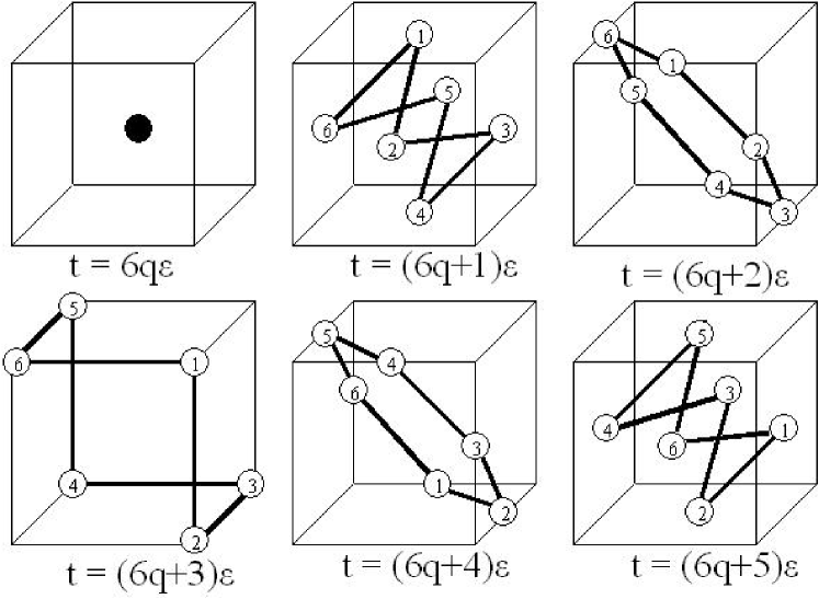
Figure 2. Evolution of the six processes $X_{\varepsilon}^{j}(n\varepsilon)$.

The evolution of the six processes ${\large X}_{\varepsilon}^{j}(n\varepsilon)$ visualizes in the figure 2. At time $t=6q\varepsilon$, the six points are in the center of a cube. At times $t=(6q+1)\varepsilon$ and $t=(6q+5)\varepsilon$, the six points are in the center of the six faces of this cube. At times $t=(6q+2)\varepsilon$ and $t=(6q+4)\varepsilon$, the six points are on a circle in the middle of six edges of the cube. At time $t=(6q+3)\varepsilon$, the six points are on the six vertices of the cube.

Remark 2.5.

It is possible to give more interpretations of the processes $Z_{\varepsilon}^{j}(t)$: non standard processes, fiber space, string. In the first interpretation, each process $Z_{\varepsilon}^{j}(t)$ is a non standard process in spite of the non standard analysis of Robinson [17] (field ${}^{\varepsilon}\mathbb{R}$ of Robinson built with the infinitesimal $\varepsilon$ added to $\mathbb{R}$) with $\widetilde{Z}\left(t\right)$ as standard part. In the fiber space interpretation, the process $Z_{\varepsilon}^{j}(t)$ corresponds to the total space and $\widetilde{Z}_{\varepsilon}\left(t\right)$ corresponds to the basic space.

The third interpretation of process defined by $\left(1\right)$ and $\left(2\right)$ is to consider this process as a special elastic string model. Its length at times $t=6q\varepsilon$ is equal to zero. At times $t\neq 6q\varepsilon$, it takes a finite length and the 6 points $X_{\varepsilon}^{j}(t)$ correspond to 6 points of a string. The motion of these points therefore corresponds to a vibration of the string. Moreover this interpretation suggests a sort of creation process between times $t=6q\varepsilon$ and $\left(6q+1\right)\varepsilon$ followed by an annihilation process between $\left(6q+5\right)\varepsilon$ and $6\left(q+1\right)\varepsilon.$

Definition 2.6.

The mean angular momentum of a process following (8) is given by:

$$\sigma=E_{n,j}\left(\sigma_{n}^{j}\right)=\frac{1}{36}\sum_{n=6q}^{6q+5}\sum_{j=1}^{6}\sigma_{n}^{j}\text{ \ \ {with}}$$

$$\sigma_{n}^{j}=r_{n}^{j}\wedge p_{n}^{j}\text{ , \ }r_{n}^{j}={\large X}_{\varepsilon}^{j}(n\varepsilon)=\widetilde{r}_{n}+\sqrt{\frac{3\hslash\varepsilon}{8m}}\left(s^{n}u^{j}-u^{j}\right)\text{ }$$

$$\text{{and }\ }p_{n}^{j}=m\frac{r_{n+1}^{j}-r_{n}^{j}}{\varepsilon}=m\frac{\widetilde{r}_{n+1}-\widetilde{r}_{n}}{\varepsilon}+\sqrt{\frac{3\hslash m}{8\varepsilon}}\left(s^{n+1}u^{j}-s^{n}u^{j}\right).$$

Using  $\sum_{j=1}^{6}s^{n}u^{j}=0$  for all n, it follows that

$$\ \sigma=\widetilde{r}\wedge m\widetilde{v}+\frac{1}{16}\hslash\sum_{j=1}^{6}\left(u^{j}\wedge su^{j}\right)$$

with $\widetilde{r}=\frac{1}{6}\sum_{n=6q}^{6q+5}\widetilde{r}_{n}$ and $\widetilde{v}=\widetilde{v}\left(6\left(q+1\right)\varepsilon\right).$

For instance, for $s=s_{1}$, that is for the permutation defined by the sequence of the 6 vertices: $u^{1}=\left\{-1,-1,-1\right\}$, $u^{2}=\left\{-1,-1,+1\right\}$, $u^{3}=\left\{1,-1,1\right\}$, $u^{4}=\left\{1,1,1\right\}$, $u^{5}=\left\{1,1,-1\right\}$, $u^{6}=\left\{-1,1,-1\right\}$, we have

$$\sum_{j=1}^{6}\left(u^{j}\wedge s_{1}u^{j}\right)=\left\{-2,2,0\right\}+\left\{0,2,2\right\}+\left\{-2,0,2\right\}+\left\{-2,2,0\right\}$$

$$+\left\{0,2,2\right\}+\left\{-2,0,2\right\}=8\left\{-1,1,1\right\}$$

and then:

$$\sigma_{x}=m\left(y\widetilde{v}_{z}-z\widetilde{v}_{y}\right)-\frac{\hslash}{2}\text{, \ }\sigma_{y}=m\left(z\widetilde{v}_{x}-x\widetilde{v}_{z}\right)+\frac{\hslash}{2}\text{ }$$

$$\text{ and \ \ }\sigma_{z}=m\left(x\widetilde{v}_{y}-y\widetilde{v}_{x}\right)+\frac{\hslash}{2}.$$

We deduce the following theorem:

Theorem 2.7.

For any $\varepsilon>0$ and for $s=s_{1}$, the real part of process defined by $\left(1\right)\left(2\right)$ has a mean intrinsic angular momentum of components: $s_{x}=+\frac{\hslash}{2},s_{y}=-\frac{\hslash}{2},s_{z}=-\frac{\hslash}{2}$. The 7 other combinations $\left(\pm\frac{\hslash}{2}\right)$ are given by the 7 other permutations of $S$.

Let be $\widetilde{x}_{\varepsilon}(n\varepsilon)$ the real mean position on the $x$ axis of the particle at time $n\varepsilon$ (with $n=6q+r$) and $m\widetilde{v}=m\widetilde{v}\left(6(q+1)\varepsilon\right)$ the real mean momentum. The calculation of standard deviations $\triangle x$ and $\Delta p_{x}$ of the position and of the momentum on the x axis, at time $n\varepsilon$ with $n=6q+w$ $\ \left(\left|w\right|\leq 3\right)$, yields:

$$\left(\Delta x\right)_{n\varepsilon}=\sqrt{\frac{1}{6}\sum_{j}\left(r_{n}^{j}-\widetilde{r_{n}}\right)_{x}^{2}}=\sqrt{\frac{\hslash\varepsilon}{2m}}\sqrt{\left|w\right|}$$

$$\left(\Delta p_{x}\right)_{n\varepsilon}=\sqrt{\frac{1}{6}\sum_{j}\left(p_{n}^{j}-\widetilde{p_{n}}\right)_{x}^{2}}=\sqrt{\frac{\hslash m}{2\varepsilon}}$$

For exemple, we have for $s=s_{1}$ and $n=6q+1:$

$$\left(\Delta x\right)_{n\varepsilon}=\sqrt{\frac{3\hslash\varepsilon}{8m}}\sqrt{\frac{1}{6}\sum_{j}\left(s_{1}u^{j}-u^{j}\right)_{x}^{2}}$$

$$=\sqrt{\frac{3\hslash\varepsilon}{8m}}\sqrt{\frac{1}{6}\left(2^{2}+2^{2}\right)}=\sqrt{\frac{\hslash\varepsilon}{2m}}$$

and

$$\left(\Delta p_{x}\right)_{n\varepsilon}=\sqrt{\frac{3\hslash m}{8\varepsilon}}\sqrt{\frac{1}{6}\sum_{j}\left(s_{1}^{2}u^{j}-s_{1}u^{j}\right)_{x}^{2}}$$

$$=\sqrt{\frac{3\hslash m}{8\varepsilon}}\sqrt{\frac{1}{6}\left(2^{2}+2^{2}\right)}=\sqrt{\frac{\hslash m}{2\varepsilon}}.$$

We deduce the second theorem:

Theorem 2.8.

For any $\varepsilon>0$ and for any $s$, the real part of process defined by $\left(1\right)\left(2\right)$ verifies the Heisenberg inequalities at any point not located on the basic trajectory (i.e. for any $\ t=n\varepsilon\neq 6q\varepsilon$):

(9) $$\left(\Delta x\right)_{n\varepsilon}\cdot\left(\Delta p_{x}\right)_{n\varepsilon}\geq\frac{\hslash}{2}.$$

Let us show that the non commutation relations of the type

$$\widehat{p}_{x}x-x\widehat{p}_{x}=-i\hslash$$

can be interpreted as the non temporal commutation of $p_{x}\left(t\right)$ and $x\left(t\right)$. Accordingly, we calculate the mean of $p_{x}\left(t+\varepsilon\right)x\left(t\right)-x\left(t+\varepsilon\right)$ $p_{x}\left(t\right)$:

$$E\left(p_{x}\left(t+\varepsilon\right)x\left(t\right)-x\left(t+\varepsilon\right)p_{x}\left(t\right)\right)=$$

$$=E_{n,j}\left(1+i\right)^{2}\left(\left(p_{n+1}^{j}\right)_{x}\left(r_{n}^{j}\right)_{x}-\left(r_{n+1}^{j}\right)_{x}\left(p_{n}^{j}\right)_{x}\right)$$

where $r_{n}^{j}$ and $p_{n}^{j}$ are defined in definition 3. We then obtain the desired result:

Theorem 2.9.

For any $\varepsilon>0$ and for any $s$, the process defined by $\left(1\right)\left(2\right)$ verifies the non temporal commutativity relation

$$E\left(p_{x}\left(t+\varepsilon\right)x\left(t\right)-x\left(t+\varepsilon\right)p_{x}\left(t\right)\right)=-i\hslash.$$

Moreover, we verify also that

$$E\left(p_{x}\left(t+\varepsilon\right)y\left(t\right)-y\left(t+\varepsilon\right)p_{x}\left(t\right)\right)=0.$$

Let be $f\left(x,t\right)$ an application of class $C^{2}$ of $\mathbb{C}^{3}\times\mathbb{R}$ in $\mathbb{C}$ and $Z_{\epsilon}^{j}\left(t\right)$ a process defined by (1) and (2). We denote the complex Dynkin operator, previously introduced by Nottale [16] under the name of ”quantum covariant derivative”:

(10) $$D=\frac{\partial}{\partial t}+\mathcal{V}\cdot\triangledown-i\frac{\hslash}{2m}\triangle$$

Lemma 2.10.

For any $\varepsilon>0$ and for any $s$, the process $Y_{\varepsilon}\left(t\right)$ defined by

(11) $$Y_{\epsilon}\left(t\right)=E_{j}f(Z_{\epsilon}^{j}\left(t\right),t)=\frac{1}{6}\ \sum_{j}\left(f\left(Z_{\epsilon}^{j}\left(t\right),t\right)\right)$$

with $Z_{\epsilon}^{j}\left(t\right)$ based on (1) and (2), verifies for any integer $q$:

(12) $$Y_{\epsilon}\left(6q\epsilon\right)-Y_{\epsilon}\left(\left(6q-1\right)\epsilon\right)=Df\left(\widetilde{Z}\left(6q\epsilon\right),6q\epsilon\right)\epsilon+o\left(\epsilon\right).$$

Proof: First, we have $Y_{\epsilon}\left(6q\epsilon\right)=f\left(\widetilde{Z}\left(6q\epsilon\right),6q\epsilon\right)$. Using $\left(5\right)$ and $\sum_{j}s^{n}u^{j}=0$, we find for all $t=n$ $\epsilon$

$$E_{j}f(Z_{\epsilon}^{j}\left(t\right),t)=f(\widetilde{Z}_{\epsilon}(t),t)+$$

$$+\frac{3i\hslash}{8m}\epsilon E_{j}\left\{\sum_{k,l}\frac{\partial^{2}f}{\partial x_{k}\partial x_{l}}\left(s^{n}u^{j}-u^{j}\right)_{k}\left(s^{n}u^{j}-u^{j}\right)_{l}\right\}+o\left(\epsilon\right).$$

For $n=6q-1$,

$$E_{j}\left(s^{n}u^{j}-u^{j}\right)_{k}\left(s^{n}u^{j}-u^{j}\right)_{l}=\frac{4+4}{6}\delta_{kl}$$

and the calculation of the last term of $E_{j}f(Z_{\epsilon}^{j}\left(t\right),t)$ gives $\frac{3i\hslash}{8m}\epsilon\frac{8}{6}\Delta f$. Then we deduce

$$Y_{\epsilon}\left((6q-1)\epsilon\right)=f(\widetilde{Z}_{\epsilon}((6q-1)\epsilon),(6q-1)\epsilon)+$$

$$+i\frac{\hslash}{2m}\epsilon\Delta f(\widetilde{Z}_{\epsilon}((6q-1)\epsilon),(6q-1)\epsilon)+o\left(\epsilon\right).$$

Hence, with the development to first order of $f(\widetilde{Z}_{\epsilon}((6q-1)\epsilon),(6q-1)\epsilon)$, equation $\left(12\right)$ follows. $\Box$

Remark 2.11.

The process defined by $\left(1\right)$ and $\left(2\right)$ is only an example of processes that we could build with permutation groups about $U_{R}$. We can preserve the previous properties, if we change the permutation $s$ or the step of time $\varepsilon$, between 2 positions of the basic trajectory. We will use this change in $\varepsilon$ in the remark 3.7 where we give a possible interpretation of $\varepsilon.$

The second part of the process defined by $\left(1\right)$ is discrete. There are many solutions to make this part continuous and differentiable, for example by a trajectory differentiable on the circumscribed sphere which passes through all the 6 vertices of each discrete process.

3. The Schrödinger equation

We then construct a complex analytical mechanics in the same way as the conventional analytical mechanics but with objects having a complex position $Z(t)\in\mathbb{C}^{3}$, a complex velocity $\mathcal{V}\left(t\right)\in\mathbb{C}^{3}$ and using the minimum of a complex function and complex minplus analysis, as introduced in [7], [9]. It is a generalisation for the complex functions of the idempotent analysis introduced by Maslov [13]. We recall the basic ideas in the two following definitions.

Definition 3.1.

Let a complex function $f\left(z\right)=f\left(x+iy\right)$ from $\ \mathbb{C}^{n}$ to $\mathbb{C}$ such as $f\left(z\right)=P\left(x,y\right)+iQ\left(x,y\right)$ with $P\left(x,y\right)$ continuous at $x$ and $y$, and a closed set $A\subset\mathbb{C}^{n}$ such as $A=\left\{x+iy/x\in X\subset\mathbb{R}^{n},y\in Y\subset\mathbb{R}^{n}\right\}.$ We define the minimum of $f$ for $z\in A$, if it exists, by:

$$\min_{z\in\mathit{A}}{f\left(z\right)}=\left\{f\left(z_{0}\right)\right\}$$

where $z_{0}=x_{0}+iy_{0}\in A$ and where $\left(x_{0},y_{0}\right)$ is a saddle point of

$P\left(x,y\right)$:

$$P\left(x_{0},y\right)\leq\text{\vskip 12.0pt plus 4.0pt minus 4.0pt}P\left(x_{0},y_{0}\right)\leq\text{\vskip 12.0pt plus 4.0pt minus 4.0pt}P\left(x,y_{0}\right)\text{ \ \ \ \ }\forall x\in X,\forall y\in Y.$$

If this saddle point is not unique, the complex part of $\min\left\{f\left(z\right)/z\in\mathbb{C}^{n}\right\}$ will be multivalued. It will be considered that a complex function $f(z)$ is (strictly) convex if $P\left(x,y\right)$ is (strictly) convex in $x$ and (strictly) concave in $y$.

If $f(z)$ is a holomorphic function, then a necessary condition for $z_{0}$ to be a minimum of $f(z)$ on $\mathbb{C}^{n}$is that $f^{\prime}\left(z_{0}\right)=0$. It is sufficient if $f(z)$ is also convex.

Definition 3.2.

To each complex and convex function, we associate its complex Fenchel transform $\widehat{f}\left(p\right):p\in\mathbb{C}^{n}\longmapsto\mathbb{C}$ defined by:

$$\widehat{f}\left(p\right)=\max_{z\in\mathbb{C}^{n}}{\left(p.z-f\left(z\right)\right).}$$

Using the classical Lagrange function $L(x,\dot{x},t)$, an analytical function in $x$ and $\dot{x}$, we define [7], [9] the complex Lagrange function $L(Z,\mathcal{V},t)$, when replacing $x(t)$ by the complex state $Z(t)$ and $\dot{x}(t)$ by the complex velocity $\mathcal{V}\left(t\right)$.

Definition 3.3.

For the process defined by $\left(1\right)\left(2\right)$, we define the complex action $\mathcal{S}_{\varepsilon}(Z,t)$ using the recurrence equation at time $t=6q\varepsilon$:

$$\mathcal{S}_{\varepsilon}(\widetilde{Z}_{\varepsilon}\left(t\right),t)=\min_{\mathcal{V}(t)}{\frac{1}{6}\sum_{j}\left\{\mathcal{S}_{\varepsilon}(Z_{\varepsilon}^{j}(t-\varepsilon),t-\epsilon)+L(\widetilde{Z}_{\varepsilon}\left(t\right),\mathcal{V}(t){\LARGE,}t)\epsilon\right\}}$$

in which the evolution between $Z_{\varepsilon}^{j}(t)$ and $Z_{\varepsilon}^{j}\left(t-\varepsilon\right)$ is given by the equation (1), and where the min is considered as the complex minimum for the possible complex velocity $\mathcal{V}\left(t\right)$. For $t=0$ we take:

$$\mathcal{S}_{\varepsilon}\left(Z,0\right)=\mathcal{S}^{0}\left(Z\right)\text{ \ \ \ \ \ \ }\forall Z\in\mathbb{C}^{3}$$

where $\mathcal{S}^{0}\left(Z\right)$ is a given holomorphic function.

This equation (13) can be interpreted as a new least action principle adapted to the trajectories of this type. The decision concerning the control takes place only at times $t=6q\varepsilon$, i.e. at the times corresponding to passage into the basic trajectory.

Theorem 3.4.

If the complex process defined by (1) and (2) has $L(x,\dot{x},t)=\frac{1}{2}m\dot{x}^{2}-V\left(x\right)$ as a Lagrangian function, then the complex action verifies the complex second order Hamilton-Jacobi equation:

(13) $$\frac{\partial\mathcal{S}}{\partial t}+\frac{1}{2m}\left(\triangledown\mathcal{S}\right)^{2}+V\left(Z\right)-i\frac{\hslash}{2m}\triangle\mathcal{S}=0\text{ \ \ \ \ \ \ }\forall\left(Z,t\right)\in\mathbb{C}^{3}\times\mathbb{R}^{+}$$

(14) $$\mathcal{S}\left(Z,0\right)=\mathcal{S}^{0}\left(Z\right)\text{ \ \ \ \ \ \ }\forall Z\in\mathbb{C}^{3}$$

Proof: For the proof, we suppose that $\mathcal{S}_{\varepsilon}(Z,t)$ is a very smooth function on $\varepsilon$ and holomorphic at $Z$ and C¹ at $t.$ By the lemma 2.10, we have

$$\frac{1}{6}\sum_{j}\left\{\mathcal{S}_{\varepsilon}(Z_{\varepsilon}^{j}(t-\varepsilon)\right\}=\mathcal{S}_{\epsilon}(\widetilde{Z}\left(t\right),t)-D\mathcal{S}_{\varepsilon}(\widetilde{Z}\left(t\right),t)+o(\varepsilon).$$

Whence, we deduce at point $\left(Z,t\right)$ the following equation:

(15) $$\frac{\partial\mathcal{S}_{\epsilon}}{\partial t}=\min_{\mathcal{V}}{\left(L(Z,\mathcal{V}{\LARGE,}t)-\mathcal{V}\cdot\triangledown\mathcal{S}_{\epsilon}+i\frac{\hslash}{2m}\triangle\mathcal{S}_{\epsilon}+o\left(\epsilon\right)\right)}.$$

Using complex Fenchel transform of $L(Z,\mathcal{V},t)$ in $\left(16\right)$ and doing $\epsilon\rightarrow$ 0${}^{+},$ we obtain $\left(13\right)$.$\Box$

If we take for wave function $\Psi=e^{i\frac{\mathcal{S}}{\hslash}}$ and apply the restriction of $\left(14\right)\left(15\right)$ to the real part of Z , the theorem 3.4 becomes:

Theorem 3.5.

If the complex process defined by (1)(2) has $L(x,\dot{x},t)=\frac{1}{2}m\dot{x}^{2}-V\left(x\right)$ for Lagrangian function, then the wave function $\Psi$ verifies the Schrödinger equation:

$$i\hslash\frac{\partial\Psi}{\partial t}=\mathcal{-}\frac{\hslash^{2}}{2m}\triangle\Psi+V(X)\Psi\qquad\forall(X,t)\in\mathbb{R}^{3}\times\mathbb{R}^{+}$$

$$\Psi(X,0)=\Psi^{0}(X)\qquad\forall X\in\mathbb{R}^{3}.\Box$$

As $L(Z,\mathcal{V},t)=\frac{1}{2}m\mathcal{V}^{2}-V\left(Z\right)$, the minimum of (15) is obtained with $m\mathcal{V-\nabla S}_{\varepsilon}=0$. Then we have

(16) $$\mathcal{V}\left(t\right)=\frac{\triangledown\mathcal{S}}{m}$$

By breaking down $\mathcal{S}(X,t)$ into its real and imaginary parts, $\mathcal{S}(X,t)=S(X,t)-\frac{i\hslash}{2}\ln\rho(X,t)$, because the wave function is also written as $\Psi=\rho e^{i\frac{S}{\hslash}}$, we can deduce that the real basic trajectory $\widetilde{X}(t)$ verifies the classical differential equation:

(17) $$\frac{d\widetilde{{\large X}}(t)}{dt}=\frac{\nabla S}{m},\text{ \ \ \ \ \ \ \ \ \ }\widetilde{{\large X}}(0)={\large X}_{0}.$$

This is the trajectory proposed by de Broglie $\left[4\right]$ and Bohm $\left[1\right]$.

Theorem 3.6.

If the complex process defined by (1) and (2) has $L(x,\dot{x},t)=\frac{1}{2}m\dot{x}^{2}-V\left(x\right)$ for Lagrangian function, then the real part of the basic trajectory follows the trajectory proposed by de Broglie and Bohm.

A fundamental property of this trajectory is that the density of probability $\varrho(x,t)$ of a family of particles satisfying (18), and having a probability density $\rho_{0}\left(x\right)$ at initial time, verifies the Madelung continuity equation:

(18) $$\frac{\partial\varrho}{\partial t}+div(\varrho\frac{\nabla S}{m})=0$$

so that the trajectories are consistent with the Copenhagen interpretation, cf. by exemple $\left[5\right]$.

Remark 3.7.

The most natural hypothesis for the choice of $\varepsilon$ is to link it to the de Broglie wavelength. Now, the internal motion of the process defined by $\left(1\right)$ and $\left(2\right)$ has a period of $6\varepsilon.$ Thus, it is possible to identify this period to the frequency of de Broglie and to put:

(19) $$6\varepsilon=T=\frac{\lambda_{dB}}{v}=\frac{h}{mv^{2}}$$

4. Conclusion

There are some questions about this model. What is the sense of the imaginary velocity? Is it the good model for the Schrödinger equation?

The complex velocity $\mathcal{V}\left(t\right)$ of the process, given by (16), is written as:

(20) $$m\mathcal{V}\left(t\right)=\nabla S-i\nabla\log\rho\frac{\hbar}{2}.$$

The original velocity proposed by de Broglie and Bohm is the real part $v(t)$ of  $\mathcal{V}\left(t\right)$

(21) $$mv\left(t\right)=\nabla S.$$

However, it is possible to show, cf.[12] and [10], that for particles with a constant spin s, as it is the case in the Schrödinger approximation, the Dirac equation implies that the momentum of a particle must be given by:

(22) $$m\mathcal{V}\left(t\right)=\nabla S+\nabla\log\rho\times\mathbf{s}$$

where the spin-dependant current is the Gordon current. The equation (21) is relevant only to spin-0 particles. This spin-dependant term was often suggested, cf. [2], [11], but only in the context of the Pauli equation and not the Schrödinger equation. This term is naturally obtained from Dirac equation and this representation in a Clifford algebra or the quaternion algebra. The momentum given by (22) has been recently valided, cf. [3] and [10], for hydrogen eigenstates.

Because $\mathbf{s=}\frac{\hbar}{2}\mathbf{u}$ (with $\mathbf{u}$ unitary), we can consider the equation (20) as the projection on the complex field of the equation (22) where

$$\nabla S+\nabla\log\rho\times\mathbf{s}$$

is the gradient of the quaternion

$$S+log\rho\mathbf{s}$$

as

$$\nabla S-i\nabla\log\rho\frac{\hbar}{2}$$

is the gradient of the complex number

$$S-i\log\rho\frac{\hbar}{2}.$$

We can conclude that the process defined by $\left(1\right)$ and $\left(2\right)$ is only a first approximation on the complex field of a more general model, certainly based on a Clifford algebra or the quaternion algebra.

References

[1]
Bohm D.J., 1952: A suggested interpretation of the quantum theory
in terms of”hidden” variables. Physical Review,
85, 166-193.
[2]
Bohm D., and Hiley B.J., 1993: The Undivided Universe.
Routledge, London and New York.
[3]
Colijn C., and Vrscay E.R., 2002: Spin-dependent Bohm trajectories
for hydrogen eigenstates. Physics Letters A300,
334-340.
[4]
de Broglie, 1927: La mécanique ondulatoire et la structure de la
matière et du rayonnement. Le Journal de Physique et le
radium. série 6, Vol. 8, n, 225-241.
[5]
d’Espagnat B., 1983: In Search of Reality. Springer,
New-York.
[6]
Feynman R.P., and Hibbs A.R., 1965: Quantum Mechanics and
Path Integrals. Mc Graw-Hill, New York.
[7]
Gondran M., 2001: Calcul des variations complexe et solutions
explicites d’équations d’Hamilton-Jacobi complexe.
C.R.Acad.Sci., Paris, 332, sérieI, 677-680.
[8]
Gondran M., 2001: Processus stochastique non standard en
mécanique. C.R.Acad.Sci., Paris, 333, sérieI,
593-598.
[9]
Gondran M., and Hoblos R., 2003: Complex calculus of variations.
Kybernetika Max-Plus special issue, 39, number
2.
[10]
Gondran M., and Gondran A., 2003: Revisiting the Schrödinger
Probability current. quant-ph/0304055v1.
[11]
Holland P.R., 1993: The quantum Theory of Motion.
Cambridge University Press.
[12]
Holland P., 1999: Uniqueness of paths in quantum mechanics. Phys.
Rev.A 60 4326.