Alternative Method for Quantum Feedback-Control

Abstract

A new method for doing feedback control of single quantum systems was proposed. Instead of feeding back precisely the process output, a cloning machine served to obtain the feedback signal and the output. A simple example was given to demonstrate the method.

I Introduction

It is a dream for both theorists and experimentalists to be able to control single quantum systems, in particular quantum gates for quantum computing. Uchiyama described how to achieve open-loop control for spin-boson model in the first day of the symposiumU . Among interesting works on open loop controls, Viola and Lloyd introduced quantum bang-bang controlVL , whereas Mancini et al. considered stochastic resonance to control quantum systemsMVBT . However, as in classical control theories, open-loop control is of limited use because in most cases it is merely a blind control.

Feedback control is not only experimentally difficult, but even theoretically impossible, because a measurement at the output collapses the system’s coherenceVN . Wiseman made many attempts to achieve feedback control, based mainly on the homodyne method of detectionWMW ; WM ; WWM . Doherty et al. used state estimation methodsDHJMT . These methods with some measurements at the output stage to have feedback signals can be summarized as shown in Fig.(1a). However, are such measurements necessary? Recent works on quantum information theories indicate that having signals need not destroy coherence.

In this paper the idea of feeding back precisely the process output is renounced. Instead, a quantum cloning machine is placed at the output side, as shown in Fig.(1b). According to quantum-cloning theorems, it is possible to make either imperfect copies with unity probabilityBH ; C or perfect copies with probability less than unityDG . In the later case, a measurement is necessary, whereas the former cloning machine, which can be decomposed into rotations and controlled NOTs gates, does not involve measurementBBHB . The former approach relies on adding some ancillary quantum system in a known state and unitarily evolving the resulting combined system. Simply stated, a cloning machine is a device to split the information of the input state.

When the Bužek and Hillery cloning machine is applied at the process output, although the feedback and output of the controlled process become imperfect, as long as the system is controllable, so that the system can be steered to any state desired, and observable, so that the system can be monitored, it made no difference for controlling. We are no more than feeding back a transformed output. For the feedback loop the cloner acts like an actuator (a device added to the feedback loop to alter the system’s controllability and observability) while for the output it distorted the output. Although the controllability and the observability of the system are modified, the coherence of the output can be preserved. An analogy is that having a colleague who is invariably half-hour late for any meeting is immaterial. As long as she arrives, it makes no difference, for all practical purposes.

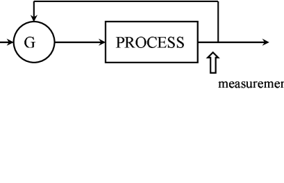
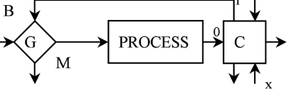
Figure 1: Comparison of standard (classical or coherent) feedback control scheme, (a), and the proposed control scheme, (b). Instead of feedback the precise process output, we feed back the cloned output and output a cloned process state. The cloner, $C$, has three pairs of input and output of which ”0” is the input state, ”1” is the cloned state, and ”x” is the ancilla (the cloning machine). For simplicity, actuators are taken to be an unity function, which made no change to the feedback state, without lost of generality.

II method

The simplest actuator is a transformation that does nothing, which Wiseman called ’simple feedback’. In practice, one can adjust the actuator function to achieve system controllability and observability as in classical control theories, which is an engineering problem.

For a mixed input state, the output state of the cloning machine reads,

$${\rho}_{0,1}^{(out)}=\frac{2}{3}{\rho}^{(in)}+\frac{1}{6}{I},$$ (1)

in which $I$ is the identity matrix. The Bloch vector shrinks by a factor of $2/3$.

We can perform logical operations for the cloned feedback state, $B$, with the input state, $I$, to obtain the process input state, $M$.

In a control theory, we suppose a knowledge of only the desired state and our input signal; intermediate states, such as the process input, are supposed to be unknown. A matching condition at the process output, or any other junction of the system, such as the process input, fixes the unknowns in ${\rho}^{(in)}$. Controllability and observability follow if this input-output mapping is one-to-one.

In conventional physics or engineering practice, a dynamic process is represented by a differential equation such as a master equation. However, as an equation of this kind can be written in terms of quantum operations, we can ignore the detail and formulate the process in turns of quantum operationsNC .

In the operator-sum formalism, a process defined by an input density matrix $\rho_{M}$, and an output density matrix $\rho_{0}$, with the process described by a quantum operation, ${\cal P}$,

$$\rho_{M}\stackrel{{\scriptstyle{\cal P}}}{{\rightarrow}}\rho_{0}.$$ (2)

${\cal P}$ can be rewritten as a completely positive linear transformation acting on the density matrix

$${\cal P}(\rho_{M})=\sum_{i}P_{i}\rho_{M}P_{i}^{\dagger}\;,$$ (3)

in which the $P_{i}$ satisfy the completeness relation

$$\sum_{i}P_{i}^{\dagger}P_{i}=I\;,$$ (4)

or equivalently $\mbox{Tr}[{\cal P}(\rho_{M})]=1$.

This way of treating the process is elegant. Furthermore, we can treat the cloning machine consistently.

III Example

As an example, we consider the process of a two-level atom coupled to the vacuum undergoing spontaneous emission. The coherent part of the atom’s evolution has a Hamiltonian $H=-\omega\sigma_{z}/2$, in which $\omega$ is the energy difference of the atomic level. The emission process is described by an Lindblad operator $\sqrt{\gamma^{{}^{\prime}}}\sigma_{-}$, in which $\sigma_{-}=\left|0\right\rangle\left\langle 1\right|$ is the atomic lowering operator, and $\gamma^{{}^{\prime}}$ is the rate of spontaneous emission. The master equation reads,

$$\dot{\rho^{{}^{\prime}}}=-i[H,\rho^{{}^{\prime}}]+\gamma^{{}^{\prime}}\left[2\sigma_{-}\rho^{{}^{\prime}}\sigma_{+}-\sigma_{+}\sigma_{-}\rho^{{}^{\prime}}-\rho^{{}^{\prime}}\sigma_{+}\sigma_{-}\right],$$ (5)

with $\sigma_{+}=\sigma_{-}^{\dagger}$. The solution of this equation in the interaction picture can be written in the operator-sum formalism, after a change of variable $\rho(t)=\exp(iHt)\rho^{{}^{\prime}}(t)\exp(-iHt)$ and using a Bloch vector representation for $\rho$, as

$$\rho_{0}={\cal P}(\rho_{M})=P_{0}\rho_{M}P_{0}^{\dagger}+P_{1}\rho_{M}P_{1}^{\dagger},$$ (6)

in which

$$P_{0}=\left(\begin{array}[]{cr}1&0\\ 0&\sqrt{1-\gamma}\end{array}\right),\;\;\;\;P_{1}=\left(\begin{array}[]{cr}0&\sqrt{\gamma}\\ 0&0\end{array}\right),$$ (7)

while $\gamma=1-\exp(-2t\gamma^{{}^{\prime}})$ implies the probability of losing a photon. For the suffixes of $\rho$, please refer to Fig.(1b).

The most general input state for the process can be written in terms of Bloch sphere representation as

$$\rho_{M}=\frac{1}{2}\left(I+\vec{a}\cdot\vec{\sigma}\right)={\frac{1}{2}}\left(\begin{array}[]{cr}1+a_{3}&a_{1}-ia_{2}\\ a_{1}+ia_{2}&1-a_{3}\end{array}\right)\;.$$ (8)

Here, $\vec{a}=(a_{1},a_{2},a_{3})$ is the Bloch vector of length unity or less, and $\vec{\sigma}$ is the vector of Pauli matrices. These intermediate variables are to be eliminated from the following calculations.

The action of the process on this density matrix produces

$${\cal P}(\rho_{M})=\frac{1}{2}\left(I+\vec{b}\cdot\vec{\sigma}\right)\;,$$ (9)

in which

$$\vec{b}=\left(a_{1}\sqrt{1-\gamma},a_{2}\sqrt{1-\gamma},a_{3}(1-\gamma)+\gamma\right)$$ (10)

is computed according to Eq.(3). This state can be fed into the cloner according to Eq.(1). The later state is also the output state of the system, since the cloning machine we used is symmetric.

For simplicity and demonstration, we consider a system without even the input terminal, in the first instance. Therefore, Bloch vector $2/3\vec{b}$ becomes the input Bloch vector of the process. Hence, $\vec{a}=2/3\vec{b}$ fixes the unknown variables of the system. The solution is $\vec{a}=2\vec{b}/3==(0,0,2\gamma/(1+2\gamma))$.

If one want to have an input signal to control the system, at least a two-qubit gate is needed for the gate, $G$, to combine the feedback signal and the input signal. It can be a controlled-NOT gate or a controlled-phase gate for example. Even more generally, a controlled-U gateEHI can serve. Furthermore, according to the Landauer’s principle, if one wishes the system to be reversible, the gate must has input terminals and output terminals of equal number, as shown in the figure, although the extra output signal can be discarded.

Suppose we take the input signal, $I$, having a Bloch vector $\vec{i}=(e_{1},e_{2},e_{3})$, and the feedback signal, $B$, as the control signal. The controlled-NOT gate read,

$$C_{NOT}=\left(\begin{array}[]{lccr}0&1&0&0\\ 1&0&0&0\\ 0&0&1&0\\ 0&0&0&1\end{array}\right)\;.$$ (11)

The total density matrix of the input and the feedback state is a direct product of the input density matrix, $\rho_{I}$, and the feedback density matrix, $\rho_{B}$. After they interact through $C_{NOT}$, partial trace is taken over the $I$ degree of freedom. The resulting density matrix reads

$$\mbox{Tr}_{I}(C_{NOT}\cdot\rho_{I}\otimes\rho_{B}\cdot C^{\dagger}_{NOT})={\frac{1}{2}}\left(\begin{array}[]{lr}1+{\frac{2}{3}}e_{3}(a_{3}(1-\gamma)+\gamma)&{\frac{2\sqrt{1-\gamma}}{3}}(a_{1}-ia_{2}e_{3})\\ {\frac{2\sqrt{1-\gamma}}{3}}(a_{1}+ia_{2}e_{3})&1-{\frac{2}{3}}e_{3}(a_{3}(1-\gamma)+\gamma)\end{array}\right).$$ (12)

Only one component of the input Bloch vector has an influence on the process, because the $C_{NOT}$ gate mixed the total density matrix only slightly whereas the partial trace operation eliminated all other components.

Matching Eq.(8) and Eq.(12) yields $a_{1}=a_{2}=0$, and $a_{3}=e_{3}\gamma/(3/2-e_{3}(1-\gamma))$, which fixes the unknown variables of the process. A valid Bloch vector has to be of length unity or less. Furthermore, note $\gamma$ is also less than unity. Through Eq.(10), one obtains the input-output relationship of the system: $b_{1}=b_{2}=0$, and $b_{3}=\gamma/(1-(2/3)e_{3}(1-\gamma))$. The system is controllable in the valid range of the process because the mapping between $\vec{a}$ and $\vec{i}$ is one to one. Furthermore, according to Eq.(10) the system is observable, because we can calculate the process state once we know the output state.

Similar calculation can be done if one take $I$ as the control signal.

In summary, the system considered maps states with Bloch vector $\vec{i}$ into states with Bloch vector $2/3\vec{b}$. If the mapping from $\vec{i}$ to $\vec{b}$ is one to one, by definition, the system is controllableTK . The mapping of state with Bloch vector $2/3\vec{b}$ to state with Bloch vector $\vec{a}$ is one to one signifies the system is observable.

IV discussion

Coherent feedback is formulated without using adiabatic elimination as Wiseman did. Our method indicated that, although the system cannot be divided, the information can. Therefore part of the output information is feed back for control purposes.

This work is a synergy of two fields in modern science, namely, automatic control theories and quantum-cloning theories. As Bruß et al. mentioned, presently quantum-cloning theories have been mainly of academic interestsBCL . A concrete example of the application of cloning theory is presented here.

In the example given, one has the freedom to either feedback the ancilla or one of the cloned copy, since the ancilla also contains the process informationBCL . According to the figure, their roles are similar.

The input control signal need not be another unknown quantum stateJAZB . It can be a quantum system in its eigenstate. We can change other parameters, such as time, for controlling. The details depend on the design of the system. On the other hand, an unknown state controlling another unknown state is not necessarily useless: A NOT-gate is an exampleB . In the same way we can design gates that switch the quantum state to a particular state. For instance, a gate that always rotates the input state by 45 degree. A control system which incorporated 45, 90, 135 degrees of rotation, with selection is another way to achieve quantum control.

With a quantum feedback system formulated in this way, many recent results in quantum information sciences are applicable. For instance, the system can be considered as a channel; it entropy exchange can be calculated and the uncertainty principle derivedTL .

Our formalism does suffer from some deficiencies: Firstly, the outputs of the cloner are likely to entangled with themselves or with the ancillaBM . We assume this does not happen presently. Secondly, because the operator-sum formalism ignores the detail evolution of the system, we can take no time lag between various components into account. The evolution time of any component must be finiteGLM . The entanglement cannot be eliminated in view of the second point because entanglement serves to accelerate the evolution. However, the time lag problem only makes difference at the design stage. The basic method for doing quantum feedback control is unchanged.

For the control scheme proposed by LloydL , he found quantum control with coherent feedback often do not distinguish between sensors and actuators. This is probably because of the models he considered are pathological. In conventional control theories, there is always an input control signal to be mixed with the feedback signal. Therefore the roles of the process and the actuator are made asymmetric. However, in Lloyd’s examples this input signal is missing.

Recently Simon et al. proposed doing quantum cloning via stimulated emissionSWZ ; KSW . In view of our proposal, this recently realized cloning machine appears to be part of Warszawski and Wiseman’s feedback control systemWW in that they all have feedback in one mode which coupled to another mode for output. Perhaps their device has a cloner implicitly built-in?

As quantum-cloning machine has been realized recentlyLLHZGJ ; MMB ; LSHB ; CJFSMPJ , and a method for making cloning machine for cavity QED is proposedMOR , the feedback control method proposed herein should be verifiable.

Finally, I thank Dr. Giyuu Kido, chairman of APF8, and the organization committee for generous support and hospitality during my visit to NIMS.

References

- (1) C. Uchiyama, Synchronized Pulse Control of Decoherence, in the 8th International Symposium on Advanced Physical Fields, this issue, quant-ph/0303144; Phys. Rev. A, 66, 032313 (2002).
- (2) L. Viola and S. Lloyd, Phys. Rev. A, 58, 2733 (1998).
- (3) S. Mancini, D. Vitali, R. Bonifacio, and P. Tombesi, Europhys. Lett. , 60, 498 (2002).
- (4) J. von Neumann, Mathematical Foundations of Quantum Mechanics (Princeton University Press, 1955).
- (5) H. M. Wiseman, S. Mancini, and J. Wang, Phys. Rev. A, 66, 013807 (2002).
- (6) H. M. Wiseman and G. J. Milburn, Phys. Rev. Lett., 70, 548 (1993).
- (7) J. Wang, H. M. Wiseman, and G. J. Milburn, Chem. Phys., 268, 221 (2001).
- (8) A. C. Doherty, S. Habib, K. Jacobs, H. Mabuchi, and S. M. Tan, Phys. Rev. A, 62 012105 (2000).
- (9) V. Bužek and M. Hillery, Phys. Rev. A, 54, 1844 (1996); Universal optimal cloning of qubits and quantum registers, in Quantum Computing and Quantum Communications (Springer Notes in Computer Science, 1509) quant-ph/9801009. See also V. Bužek and M. Hillery, Physics World, 14, No.11, 25 (2001).
- (10) N. J. Cerf, Phys. Rev. Lett., 84, 4497 (2000).
- (11) L.-M. Duan and G.-C. Guo, Phys. Rev. Lett., 80, 4999 (1998).
- (12) V. Bužek, S. L. Braunstein, M. Hillery, and D. Bruß, quant-ph/9703046 (1997).
- (13) M. A. Nielsen and I. L. Chuang, Quantum Computation and Quantum Information, (Cambridge University Press, Cambridge, 2000) Chapter 8. Section 4, in particular. Strictly, not all process can be written in this way, c.f. the same book or A. S. Holevo, quant-ph/0204077.
- (14) A. Ekert, P. Hayden, and H. Inamori, quant-ph/0011013, lectures given at les Houches Summer School on ”Coherent Matter Waves”, July-August 1999.
- (15) T. Kailath, Linear System, (Prentice Hall, 1996).
- (16) D. Bruß, J. Calsamiglia and N. Lütkenhaus, Phys. Rev. A, 63, 042308 (2001).
- (17) D. Janzing, F. Armknecht, R. Zeier, and Th. Beth, Phys. Rev. A, 65, 022104 (2002) mentioned this problem, although they did not tackle it.
- (18) F. De Martini, V. Bužek, F. Sciarrino, and C. Sias, Nature, 419, 815 (2002)
- (19) H. Touchette and S. Lloyd, Phys. Rev. Lett., 84 1156 (2000).
- (20) D. Bruß and C. Macchiavello, quant-ph/0212059.
- (21) V. Giovannetti, S. Lloyd, and L. Maccone, quant-ph/0206001.
- (22) S. Lloyd, Phys. Rev. A, 62, 022108 (2000), expanded and modified version of quant-ph/9703042.
- (23) J. Kempe, C. Simon, and G. Weihs, Phys. Rev. A, 62 032302 (2000).
- (24) C. Simon, G. Weihs, and A. Zeilinger, Phys. Rev. Lett., 84, 2993 (2000).
- (25) P. Warszawski and H. M. Wiseman, quant-ph/0005127.
- (26) W.-L. Li, C.-F. Li, Y.-F. Huang, Y.-S. Zhang, Y. Jiang, G.-C. Guo, Phys. Rev. A, 64, 012315 (2001)
- (27) F. De Martini, V. Mussi, and F. Bovino, Optic. Comm., 179, 581 (2000).
- (28) A. Lamas-Linares, C. Simon, J. C. Howell, and D. Bouwmeester, Science, 296 712 (2002).
- (29) H. K. Cummins, C. Jones, A. Furze, N. F. Soffe, M. Mosca, J. M. Peach, and J. A. Jones, Phys. Rev. Lett., 88 187901 (2002).
- (30) P. Milman, H. Ollivier, and J. M. Raimond, Phys. Rev. A, 67, 012314 (2003).