Quantum computation based on d-level cluster state

Abstract

The concept of qudit (a d-level system) cluster state is proposed by generalizing the qubit cluster state (Phys. Rev. Lett. 86, 910 (2001)) according to the finite dimensional representations of quantum plane algebra. We demonstrate their quantum correlations and prove a theorem which guarantees the availability of the qudit cluster states in quantum computation. We explicitly construct the network to show the universality of the one-way computer based on the defined qudit cluster states and single-qudit measurement. And the corresponding protocol of implementing one-way quantum computer can be suggested with the high dimensional “Ising” model which can be found in many magnetic systems.

I Introduction

Quantum computers can process computational tasks that are intractable with classical computers. The reason lies in the fact that quantum computing systems composed by qubits (two-level quantum systems) possess mysterious quantum coherence, such as entanglement (or quantum correlation), which has no counterpart in the classical realm Ni . Recently, an important kind of entangled states, cluster states Bri , was introduced with remarkable property—the maximal connectedness, i.e., each pair of qubits can be projected onto maximally entanglement state with certainty by single-qubit measurements on all the other qubits. More surprisingly, it was shown that the cluster states can be used to build a one-way universal quantum computer, in which all the operations can be implemented by single-qubit measuments only Rau . As one of the key elements to realize such a scalable quantum computer, a celebrated theorem proved by R. Raussendorf and H. J. Briegel provides a simple criterion for the functioning of gate simulations on such quantum computer Rau1 . It was pointed out that the protocol of cluster state computers can be easily realized in practical physical systems since the creation of the cluster states needs only Ising-type interactions Bri . In fact, it has been demonstrated that the Hamiltonian with such interactions can be easily found in the solid state lattice systems with proper spin-spin interactions Bri , even in the system for cold atoms in optical lattices Du .

Theoretically, it is natural to ask whether the concept of cluster states would have its counterpart in higher dimensional Hilbert space, i.e., the qudits cases, since most of the available physical systems can not be treated as a two-level systems even in an approximate way. The answer to this question is affirmative. Using a pair of non-commutative operators $X$ and $Z$, which will be identified with the $d$ dimensional irreducible representations of Manin’s quantum plane algebra (QPA) in Sec. II Sun , we find that the qudit cluster states $|\phi\rangle_{\mathcal{C}}$ can be defined as a common eigenstate of the tensor product operators

$$X^{{\dagger}}_{a}\bigotimes\limits_{b\in{\mathtt{nbgh}}(a)}Z_{b},$$ (1)

where the lower indexes $a$ and $b$ denote qudit $a$ and qudit $b$ in the cluster, and index $b$ is taken in the neighborhood of index $a$ depending on the cluster structure. Based on this definition of qudit cluster states, we further show that we can build an one way universal quantum computer by explicitly demonstrating how to construct all single qudit unitary gates and one imprimitive two-qudit gate.

We organize our paper as follows: We first briefly review the finite dimensional representations of quantum plane algebra in Sec. II, which provides the main mathematical tools in this article. As a non-trivial generalization of the qubit cluster state, the qudit cluster state is defined according to the quantum plane algebra, and its essential properties of quantum correlations are analyzed in Sec. III. In Sec.IV, the one-way quantum computer based on qudit cluster states is proposed with crucial supports from the proof of a central theorem. Similar to that for qubit case Rau1 , this theorem guarantees the functioning of gate simulations on those computers. Its proof depends on the subtle understanding about the quantum correlations of the qudit cluster states. In Sec. V, the universality of the qudit cluster state computers is proved through the explicit construction of all the single- and one two-qudit logic gates. Finally, we give our conclusion in the last section.

II Finite dimensional representaions of quantum plane algebra

In this section, we will review the mathematics for finite dimensional representations of Manin’s quantum plane algebra, which will be the main mathematical tool to describe not only qudit cluster states but also unitary transformation on the Hilbert space. The Manin’s quantum plane is defined by

$$XZ=qZX,$$ (2)

where $q$ is a complex number. Mathematically, it can be proved that the associated algebra generated by $Z$, $X$ possesses a $d-$dimensional irreducible representation only for $q^{d}=1$ Sun . In this article, we take $q\equiv q_{d}\equiv e^{i\frac{2\pi}{d}}$. This special case is first introduced by Weyl Wey and whose completeness is first proved by Schwinger Sch . Obviously, when $d=1,\,q=1$, $X$ and $Z$ can be regarded as the ordinary coordinates of $R^{2}$ plane; When $d=2,\,q=-1$, $X$ and $Z$ can be identified with the Pauli matrices $\sigma_{x}$ and $\sigma_{z}$. In this sense $Z$ and $X$ can be regarded as the so-called “generalized Pauli operators” Bar1 ; San ; Dab ; Got ; Pat ; Kni .

In fact, when $q=q_{d}$, $Z^{d}$ and $X^{d}$ commutate with the algebra generators, so they belong to the center of QPA. The Shur’s lemma tells us $Z^{d}$ and $X^{d}$ are constants multiples of the $d-$dimensional identity matrix, i.e., $Z^{d}=zI$ and $X^{d}$ $=xI$. In general we can normalize them to the identity. Since the complex field $C$ is algebraically closed, there must exist an eigen-state $|0\rangle$, which satisfies

$$Z|0\rangle=|0\rangle.$$ (3)

According to Eq. (2), we obtain all the eigenvalue equations for operator $Z$

$$Z|k\rangle=q_{d}^{k}|k\rangle,\,(k\in Z_{d}),$$ (4)

where $|k\rangle=X^{\dagger k}|0\rangle$. This also implies

$$X|k\rangle=|k-1\rangle.$$ (5)

In the $Z$-diagonal representation, the matrices of $X$ and $Z$ are:

$$Z=\left[\begin{array}[]{cccccc}1&0&0&\cdots&0&0\\ 0&q_{d}&0&\cdots&0&0\\ \vdots&\vdots&\vdots&\ddots&\vdots&\vdots\\ 0&0&0&\cdots&q_{d}^{d-2}&0\\ 0&0&0&\cdots&0&q_{d}^{d-1}\end{array}\right],$$ (6)

$$X=\left[\begin{array}[]{cccccc}0&1&0&\cdots&0&0\\ 0&0&1&\cdots&0&0\\ \vdots&\vdots&\vdots&\ddots&\vdots&\vdots\\ 0&0&0&\cdots&1&0\\ 1&0&0&\cdots&0&0\end{array}\right].$$ (7)

From Eq. (5), we have

$$X|x(0)\rangle=|x(0)\rangle,$$ (8)

where

$$|x(0)\rangle=\frac{1}{\sqrt{d}}\sum\limits_{k=0}^{d-1}|k\rangle.$$ (9)

Similar to the eigenvalue equation of $Z$, we have

$$X|x(j)\rangle=q_{d}^{j}|x(j)\rangle,$$ (10)

where

$$|x(j)\rangle=Z^{j}|x(0)\rangle=\frac{1}{\sqrt{d}}\sum\limits_{k=0}^{d-1}q_{d}^{jk}|k\rangle.$$ (11)

Corresponding to this representation, we can also define $Z(d)$ algebra as generated by $Z$, $X$. Its all basis elements

$$B=\{Z^{j}X^{k},\,(j,k\in Z_{d})\},$$ (12)

are called unitary operator bases in Ref. Sch . The general commutation relations for any two basis elements are

$$X^{j}Z^{k}=q_{d}^{jk}Z^{k}X^{j}.$$ (13)

In addition, we can replace the generators $Z$ and $X$ with two other elements in the basis. First, Let $(m,n)$ be the greatest common factor of integers $m$ and $n$. Then if $(m_{1},n_{1})=1,\;(m_{1},n_{1}\in Z_{d})$, we can take

$$\bar{Z}=q_{d}^{-\frac{d-1}{2}m_{1}n_{1}}Z^{m_{1}}X^{n_{1}},$$ (14)

where the factor before $Z^{m}X^{n}$ makes $\bar{Z}$ have the same eigenvalues with $Z$. To maintain Eq. (2), we take

$$\bar{X}=q_{d}^{-\frac{d-1}{2}m_{2}n_{2}}Z^{m_{2}}X^{n_{2}},$$ (15)

where $(m_{2},n_{2})=1,\;(m_{2},n_{2}\in Z_{d})$, and $m_{1}n_{2}-m_{2}n_{1}=1$. From another viewpoint, $\bar{Z}$ and $\bar{X}$ defines a unitary transformation $U$

$$\bar{Z}=UZU^{\dagger},\quad\bar{X}=UXU^{\dagger}.$$ (16)

By the above definition, it is easy to check that all this kind of unitary transformations form a group. In fact, it is the so-called Clifford group, which is a useful concept in universal quantum computation.

III Qudit cluster states in quantum plane

To generalize the concept of qubit cluster states to qudit cases, we first restrict ourselves to one dimensional lattices for the sake of the conceptual simplicity. First, let us recall the definition of one-dimensional cluster states for $N$ qubits. For a $N$-site lattice, each qubit is attached to a site. As a novel multi-qubit entanglement state, the cluster state is written as

$$|\phi\rangle_{\mathcal{C}}=\frac{1}{2^{N/2}}\bigotimes\limits_{a=1}^{N}(|0\rangle_{a}+|1\rangle_{a}(\sigma_{z})_{a+1}),$$ (17)

where $(\sigma_{i})_{a}\,(i=x,y,z)$ are the Pauli matrices assigned for site $a$ in the lattice, and

$$\sigma_{z}|s\rangle=(-1)^{s}|s\rangle,\,(s\in\{0,1\}).$$

Analogy to Eq. (17), it is natural to conjuncture that the qudit cluster state in one dimension as

$$|\phi\rangle_{\mathcal{C}}=\frac{1}{d^{N/2}}\bigotimes\limits_{a=1}^{N}\left(\sum\limits_{k=0}^{d-1}|k\rangle_{a}Z^{k}_{a+1}\right),$$ (18)

where

$$Z_{a}|k\rangle_{a}=q_{d}^{k}|k\rangle_{a},\,\forall a.$$ (19)

Now we present one of our main result:

Theorem 1

The qudit cluster state in one dimension defined by Eq. (18) is a common eigen-state, with eigen-values being equal to $1$, of the operators $X^{{\dagger}}_{a}\bigotimes\limits_{b\in{\mathtt{nbgh}}(a)}Z_{b}$ , i.e.,

$$X^{{\dagger}}_{a}\bigotimes\limits_{b\in{\mathtt{nbgh}}(a)}Z_{b}|\phi\rangle_{\mathcal{C}}=|\phi\rangle_{\mathcal{C}},$$ (20)

where

$${\mathtt{nbgh}}(a)=\left\{\begin{array}[]{ll}\{2\},&a=1,\\ \{N-1\},&a=N,\\ \{a-1,a+1\},&a\notin\{1,N\}.\end{array}\right.$$ (21)

Proof. To prove this theorem, we notice that qudit cluster state (18) can be constructed in the following procedure. We first prepare a product state

$$|+\rangle=\bigotimes\limits_{a=1}^{N}|x(0)\rangle_{a},$$

then apply a unitary transformation

$$S=\prod\limits_{b-a=1}S_{ab}$$ (22)

to the state $|+\rangle$. Here $S_{ab}$ is defined by as an intertwining operator

$$S_{ab}|j\rangle_{a}|k\rangle_{b}=q_{d}^{jk}|j\rangle_{a}|k\rangle_{b}.$$ (23)

It is easy to prove

$$|\phi\rangle_{\mathcal{C}}=S|+\rangle.$$ (24)

Since $X^{{\dagger}}_{a}|+\rangle=|+\rangle$, it is easy to check

$$SX^{{\dagger}}_{a}S^{{\dagger}}|\phi\rangle_{\mathcal{C}}=|\phi\rangle_{\mathcal{C}}.$$ (25)

The next step is to prove

$$SX^{{\dagger}}_{a}S^{{\dagger}}=X^{{\dagger}}_{a}\bigotimes\limits_{b\in{\mathtt{nbgh}}(a)}Z_{b}$$

To this end, for $a,b,c\in\{1,...,N\}$, we observe that

$$S_{ab}X^{{\dagger}}_{a}S_{ab}^{{\dagger}}=X^{{\dagger}}_{a}\otimes Z_{b},$$ (26)

$$S_{ab}X^{{\dagger}}_{b}S_{ab}^{{\dagger}}=Z_{a}\otimes X^{{\dagger}}_{b},$$ (27)

$$S_{ab}X^{{\dagger}}_{c}S_{ab}^{{\dagger}}=X^{{\dagger}}_{c},\,\forall c\notin\{a,b\},$$ (28)

and

$$S_{ab}Z_{c}S_{ab}^{{\dagger}}=Z_{c},\,\forall c.$$ (29)

This completes the proof. $\Box$

Although the above proof is restricted to one dimensional cluster, it is convenient to generalize from one-dimensional qudit cluster to more complex clusters whether in two or three dimensional space. In fact, for a general cluster $C$ with one qudit on each site, the cluster state $|\phi\rangle_{\mathcal{C}}$ is defined by the following eigen-equations:

$$X^{{\dagger}}_{a}\bigotimes\limits_{b\in{\mathtt{nbgh}}(a)}Z_{b}|\phi\rangle_{\mathcal{C}}=|\phi\rangle_{\mathcal{C}}.$$ (30)

Formally, the definition of a general cluster is the same as one dimensional case. Different clusters correspond to different relations of neighbours.

Now we will discuss the properties of quantum correlations in the above cluster states under single qudit measurements. For simplicity, we still restrict ourselves to one dimensional case.

First, let us discuss how to describe a von Neumann measurement for single qudit. Although the generator $Z$ (or $X$) is not Hermitian, i.e., the eigenvalues of $Z$ (or $X$) are not real, the non-degenerate eigenstates of $Z$ (or $X$) can still form a complete orthogonal basis of $H_{d}$. Therefore they can be used to define a von Neumann measurement. For example, when we make a measurement marked by $Z$, we mean that we can obtain different results corresponding to different eigenstates of $Z$.

Next, we discuss the minimal number of single qudit measurements needed to destroy all the quantum correlations in qudit cluster states. For the one dimensional cluster state, we find all quantum entanglement will be destroyed by measuring $Z_{2a},\,(a=1,2,\cdots,[N/2])$.

Finally, we will discuss the most remarkable property - maximally connected - of qudit cluster state, i.e., each pair of qudits in the cluster can be projected onto maximally entanglement state with certainty by single-qudit measurement with all the other qudits. In fact, to project arbitrary two qudits in one dimensional cluster onto maximally entanglement state, we only need to measure $X$ for the qudits between them, and $Z$ for all the other qudits. It is easy to find that two or three dimensional qudit cluster states is also maximally connected. We only need to find a one-dimensional path connecting these two qudits and measure $Z$ for all the other qudits which are not on the path, which reduces the two or three dimensional problem to one dimension.

We now discuss the problem of physical implementation of our one-way quantum computer. Physically the qudit cluster state (18) can be created by Hamiltonian

$$H=-\hbar g\sum\limits_{(a,b)}N^{(z)}_{a}N^{(z)}_{b},\,(g>0)$$ (31)

where $(a,b)$ denotes sites $a$ and $b$ are nearest neighbors in the cluster; and $N^{(z)}$ is defined as

$$N^{(z)}=\sum\limits_{k=0}^{d-1}|k\rangle k\langle k|$$ (32)

Then we find the intertwining operator $S$ in Eq. (22) has the the explicit form

$$S=exp\left(-\frac{i}{\hbar}Ht_{\mathcal{C}}\right),$$ (33)

where the evolution time $t_{\mathcal{C}}=\frac{2\pi}{dg}$.

To associate with more familiar Hamitonian in physics, let us define the spin-$\frac{(d-1)}{2}$ operator of $z$ direction

$$s_{z}=N^{(z)}-\frac{d-1}{2}.$$ (34)

Then we can rewrite Eq. (31) as

$$H=\frac{d-1}{2}\hbar g\sum\limits_{a}\nu_{a}{(s_{z})}_{a}-\hbar g\sum\limits_{(a,b)}{(s_{z})}_{a}{(s_{z})}_{b},$$ (35)

where $\nu_{a}$ is the number of nearest neighbors for qudit $a$ in the cluster. Obviously, the interaction Hamiltonian

$$H_{I}=-\hbar g\sum\limits_{(a,b)}(s_{z})_{a}(s_{z})_{b},$$ (36)

which is the ferromagnetic Ising type interaction with spin-$\frac{d-1}{2}$.

Those kinds of Ising model, other than the usual spin-$1/2$ Ising model, has been one of the most actively studied systems in condenced matter and statistical physics due to their rich variety of critical and multicritical phenomena. For example, the spin - $1$ Ising model with nearest- neighbor interactions and a single-ion potential is know as the Blume-Emery-Griffiths (BEG) model Blu , the spin - $3/2$ Ising model was introduced to explain phase transitions in $DyVO4$ and its phase diagrams were obtained within the mean-field approximation Siv . In addition, higher spin Ising models can be associated with the magnetic properties of artificially fabricated superlattices. Such lattices consist of two or more ferromagnetic materials have been widely studied over the years, because their physical properties differ dramatically from simple solids formed from the same materials. The development of film deposition techniques has aroused great interest in the synthesis and study of superlattices in other materials. A number of experimentalKwo ; Maj ; Kre ; Cam1 and theoretical worksIzm ; Mat ; Hin ; Qu ; Fis ; Gri1 ; Sy ; Sab1 have been devoted to those directions.

IV Measurement based quantum computation with qudit

As discussed above, the qudit cluster states exhibit the same features in quantum entanglement as that for the qubit cluster states. Then a question arises naturally: Can these natures of quantum correlations be available for constructing the universal quantum computations? We will give an affirmative answer to this question in the following two sections.

In this section, we further generalize the basic concept of “single qudit quantum measurement” and the corresponding measurement based quantum computation (MBQC) on qubit clusters to that on qudit clusters. Along the line to construct MBQC for the qubit case, we will formulate the corresponding theorem which relates unitary transformation to quantum entanglement exhibited by the qudit cluster states. Quantum computations with qudit clusters inherit all basic concepts of those with qubit clusters. They include the basic procedure of simulation of any unitary gate, the concatenation of gate simulation and the method to deal with the random measurement results. Here we will give a $d$-dimensional parallel theorem as generalization of the central theorem $1$ in Ref. Rau1 .

Before formulating our central theorem, let us introduce the basic elements for quantum computing with qudit clusters. The main task of quantum computing with qudits is to simulate arbitrary quantum gate $g$ defined on $n$ qudits Hilbert space. For this purpose, the first step for quantum computing on qudit clusters is to find out a proper cluster $\mathcal{C}(g)$. Then we divide it into three sub-clusters: the input cluster $\mathcal{C}_{I}(g)$, the body cluster $\mathcal{C}_{M}(g)$, and the output cluster $\mathcal{C}_{O}(g)$. As usual we require that the input and output clusters have the same rank (i.e. the same number of qudits), $|\mathcal{C}_{I}(g)|=|\mathcal{C}_{O}(g)|=n$. Then we prepare the initial state in

$$|\Psi(\mathtt{in})\rangle_{\mathcal{C}(g)}=|\psi(\mathtt{in})\rangle_{\mathcal{C}_{I(g)}}|+\rangle_{\mathcal{C}_{M(g)}\cup\mathcal{C}_{O(g)}}.$$ (37)

In this first step of quantum computing, we entangle the qudits on the qudit cluster by using the cluster state generator $S$, i.e.,

$$|\Phi(\mathtt{in})\rangle_{\mathcal{C}(g)}=S|\Psi(\mathtt{in})\rangle_{\mathcal{C}(g)}.$$ (38)

This step brings the structure information of the qudit cluster into our computing process, and thus relates it with the corresponding qudit cluster state.

The second step is to measure all qudits on the cluster in special space-time dependent basis according to a given measurement pattern (MP). The definition of MP is given as follows.

Definition 1

A measurement pattern ${\mathcal{M}}_{{\mathcal{C}}}$ on a cluster ${\mathcal{C}}$ is a set of unitary matrixes

$${\mathcal{M}}_{{\mathcal{C}}}=\left\{u_{a}Z_{a}u_{a}^{\dagger}\,|\,\,a\in{\mathcal{C}},\,u_{a}\in SU(d)\right\},$$ (39)

which determines the one-qudit measured operators $N^{(u)}_{a}$ on ${\mathcal{C}}$, with the explicit form

$$N^{(u)}_{a}=\sum_{s=0}^{d-1}u_{a}|s\rangle_{a}s\,{{}_{a}\;\!\!}\langle s|{u_{a}}^{\dagger}.$$ (40)

If this measurement pattern $\mathcal{M}_{\mathcal{C}}$ operates on the initial state $|\Phi(\mathtt{in})\rangle_{\mathcal{C}(g)}$, the set of measurement outcomes

$$\{{s}\}_{\mathcal{C}}=\left\{{s}_{a}\in Z_{d}\,|\,\,a\in\mathcal{C}\right\}$$ (41)

is obtained. Then, modulo norm factor, the resulting state $|\Psi_{\mathcal{M}}\rangle_{\mathcal{C}}$ is given by

$$|{\Phi}_{\mathcal{M}_{\mathcal{C}}}^{\{s\}}\rangle=P^{\{s\}}_{\mathcal{M}_{\mathcal{C}}}\,|\Phi(\mathtt{in})\rangle_{\mathcal{C}(g)},$$ (42)

where the pure state projection

$$P^{\{{s}\}}_{\mathcal{M}_{\mathcal{C}}}=\bigotimes_{k\in\mathcal{C}}u_{k}|s\rangle_{k}\,{{}_{k}\;\!\!}\langle s|u^{\dagger}_{k}.$$ (43)

It is worthy pointing out that we always measure $X$ for the input qudits and $Z$ for the output, which is independent of gate $g$, i.e.,

$$\mathcal{M}_{\mathcal{C}_{I}(g)} = \{X_{i},\,i\in\mathcal{C}_{I}(g)\},$$ (44)

$$\mathcal{M}_{\mathcal{C}_{O}(g)} = \{Z_{i},\,i\in\mathcal{C}_{O}(g)\}.$$ (45)

Then we reach the final step, to associate the measurement values with the result of gate $g$ acting on the initial state.

From the above standard procedure of qudit clusters quantum computation, we learn that what is crucial for this scheme is to associate a given gate $g$ with a measurement pattern. Although by now we have no general optimal operational procedure to do this for practical problem, the following theorem provides a useful tool in realizing specific gates on the qudit clusters.

Theorem 2

Suppose that the state $|\psi\rangle_{{\mathcal{C}}(g)}=P^{\{{s}\}}_{{\mathcal{M}}_{\mathcal{C}_{M}}(g)}\,|\phi\rangle_{{\mathcal{C}}(g)}$ obeys the $2n$ eigenvalue equations

$$X_{{\mathcal{C}}_{I}(g),i}\left(UX_{i}U^{\dagger}\right)_{{\mathcal{C}}_{O}(g)}|\psi\rangle_{{\mathcal{C}}(g)} = q_{d}^{-\lambda_{x,i}}|\psi\rangle_{{\mathcal{C}}(g)}$$ (46)

$${Z^{\dagger}}_{{\mathcal{C}}_{I}(g),i}\left(UZ_{i}U^{\dagger}\right)_{{\mathcal{C}}_{O}(g)}|\psi\rangle_{{\mathcal{C}}(g)} = q_{d}^{-\lambda_{z,i}}|\psi\rangle_{{\mathcal{C}}(g)},$$ (47)

with $\lambda_{x,i},\lambda_{z,i}\in Z_{d}$ and $1\leq i\leq n$. Then, according to the above standard quantum computing procedure, we have

$$P^{{\{s\}}}_{{\mathcal{M}}_{\mathcal{C}_{I}(g)}}P^{{\{s\}}}_{\mathcal{M}_{{\mathcal{C}}_{M}(g)}}\,|\Phi(\mathtt{in})\rangle_{{\mathcal{C}}(g)}\propto(\prod|s_{i}\rangle)_{{\mathcal{C}}_{I}(g)\cup{\mathcal{C}}_{M}(g)}{|\psi({\mathtt{out}})\rangle}_{{\mathcal{C}}_{O}(g)},$$ (48)

where the input and output state in the simulation of $g$ are related via

$$|\psi({\mathtt{out}})\rangle=UU_{\Sigma}\,|\psi({\mathtt{in}})\rangle,$$ (49)

where $U_{\Sigma}$ is a byproduct operator given by

$$U_{\Sigma}=\bigotimes_{({\mathcal{C}}_{O}(g)\ni i)=1}^{n}(Z_{i})^{-\lambda_{x,i}-{s}_{i}}(X_{i})^{\lambda_{z,i}}.$$ (50)

Proof. Let us begin with the case when

$$|\psi(\mathtt{in})\rangle_{\mathcal{C}_{I}(g)}=|\{t\}\rangle_{\mathcal{C}_{I}(g)},$$ (51)

with

$$\{t\}=\{t_{1}t_{2}\cdots t_{n}\}.$$

To associate with $|\psi\rangle_{{\mathcal{C}}(g)}$, the initial input state is written as

$$|\psi(\mathtt{in})\rangle_{\mathcal{C}_{I}(g)}=(\sqrt{d})^{n}P^{\{t\}}_{\mathcal{M}^{\prime}_{\mathcal{C}_{I}(g)}}|+\rangle_{\mathcal{C}_{I}(g)},$$ (52)

where

$$\mathcal{M}^{\prime}_{\mathcal{C}_{I}(g)}=\{Z_{i},\,i\in\mathcal{C}_{I}(g)\}.$$ (53)

In terms of Eqs. (37, 38, 48, 52), we have

$$(\prod|s_{i}\rangle)_{{\mathcal{C}}_{I}(g)\cup{\mathcal{C}}_{M}(g)}{|\psi({\mathtt{out}})\rangle}_{{\mathcal{C}}_{O}(g)}\propto P^{\{s\}}_{\mathcal{M}_{\mathcal{C}_{I}(g)}}P^{\{t\}}_{\mathcal{M}^{\prime}_{\mathcal{C}_{I}(g)}}|\psi\rangle_{{\mathcal{C}}(g)}.$$ (54)

To find out the equations for the final state ${|\psi({\mathtt{out}})\rangle}_{{\mathcal{C}}_{O}(g)}$, we take $P^{\{s\}}_{\mathcal{M}_{\mathcal{C}_{I}(g)}}P^{\{t\}}_{\mathcal{M}^{\prime}_{\mathcal{C}_{I}(g)}}$ acting on both sides of Eq. (46) and Eq. (47):

$$\left(UX_{i}U^{\dagger}\right)_{{\mathcal{C}}_{O}(g)}{|\bar{\psi}({\mathtt{out}})\rangle}_{{\mathcal{C}}_{O}(g)}=q_{d}^{-s_{i}-\lambda_{x,i}}{|\psi({\mathtt{out}})\rangle}_{{\mathcal{C}}_{O}(g)},$$ (55)

$$\left(UZ_{i}U^{\dagger}\right)_{{\mathcal{C}}_{O}(g)}{|\psi({\mathtt{out}})\rangle}_{{\mathcal{C}}_{O}(g)}=q_{d}^{t_{i}-\lambda_{z,i}}{|\psi({\mathtt{out}})\rangle}_{{\mathcal{C}}_{O}(g)},$$ (56)

where the input state for $|\bar{\psi}({\mathtt{out}})\rangle$

$$|\bar{\psi}({\mathtt{in}})\rangle=X_{i}^{\dagger}|\{t\}\rangle.$$ (57)

Before drawing a conclusion, we need to check the final state is not a zero vector. In fact, from Eqs. (46) and (47), the state $U^{\dagger}|\psi\rangle_{{\mathcal{C}}(g)}$ is the simutaneous eigen-state of operators $X_{{\mathcal{C}}_{I}(g),i}X_{{\mathcal{C}}_{O}(g),i}$ and ${Z^{\dagger}}_{{\mathcal{C}}_{I}(g),i}Z_{{\mathcal{C}}_{O}(g),i}$. We can directly evaluate this state and find out that it has every components in $Z$-diagonal representation of the input part. Consequently the final state is indeed a nonzero vector. So from Eq. (55) and Eq. (56), we obtain

$$|\psi(\mathtt{out})\rangle_{{\mathcal{C}}_{O}(g)}=e^{i\eta(t)}UU_{\Sigma}\,|\{t\}\rangle_{{\mathcal{C}}_{O}(g)}.$$ (58)

To further determine the relation between the output state and the input state, let us consider the other case when

$$|\psi^{\prime}(\mathtt{in})\rangle_{{\mathcal{C}}_{I}(g)}=|+\rangle_{\mathcal{C}_{I}(g)}.$$ (59)

At this time, the final state

$$|\{s_{i}\}\rangle_{{{\mathcal{C}}_{I}(g)}\cup{{\mathcal{C}}_{M}(g)}}\,|\psi^{\prime}(\mathtt{out})\rangle_{{\mathcal{C}}_{O}(g)}=P^{{\{s\}}}_{{\mathcal{C}}_{I}(g)}({X})|\psi\rangle_{{\mathcal{C}}(g)}.$$ (60)

Let $P^{{\{s\}}}_{\mathcal{M}_{{\mathcal{C}}_{I}(g)}}$ apply on both sides of Eq. (46) and Eq. (47), we obtain

$$\left(UX_{i}U^{\dagger}\right)_{{\mathcal{C}}_{O}(g)}|\psi^{\prime}(\mathtt{out})\rangle_{{\mathcal{C}}_{O}(g)}=q_{d}^{-s_{i}-\lambda_{x,i}}|\psi^{\prime}(\mathtt{out})\rangle_{{\mathcal{C}}_{O}(g)},$$ (61)

$$\left(UZ_{i}U^{\dagger}\right)_{{\mathcal{C}}_{O}(g)}|\bar{\psi^{\prime}}(\mathtt{out})\rangle_{{\mathcal{C}}_{O}(g)}=q_{d}^{-\lambda_{z,i}}|\psi^{\prime}(\mathtt{out})\rangle_{{\mathcal{C}}_{O}(g)},$$ (62)

where the input state for $|\bar{\psi^{\prime}}(\mathtt{out})\rangle$

$$|\bar{\psi^{\prime}}(\mathtt{in})\rangle=Z^{\dagger}_{i}|+\rangle.$$ (63)

From the above equations, we obtain

$$|\psi^{\prime}(\mathtt{out})\rangle_{{\mathcal{C}}_{O}(g)}=e^{i\chi}UU_{\Sigma}\,|+\rangle_{{\mathcal{C}}_{O}(g)}.$$ (64)

Substitute Eq. (58) into Eq. (64),

$$|\psi^{\prime}(\mathtt{out})\rangle_{{\mathcal{C}}_{O}(g)}=UU_{\Sigma}d^{-\frac{n}{2}}\sum_{\{t\}}e^{i\eta(t)}\,|\{t\}\rangle_{{\mathcal{C}}_{O}(g)}.$$ (65)

Comparing Eq. (64) to Eq. (65), we obtain

$$e^{i\eta(t)}=e^{i\chi}.$$ (66)

This completes the proof.$\,\Box$

This theorem tells us that, since the cluster states have remarkable quantum correlations, which has been discussed in Sec. II, they play an essential role in the realization of arbitrary unitary gates. More precisely, as long as one cluster can be used to process a unitary gate for the cluster state, it will work for arbitrary input states. Therefore, it is sufficient to check the conditions for the cluster states, i.e., Eq. (46) and Eq. (47). To be emphasized, the special features of the above theorem arising from qudits is that it is expressed not only in terms of unitary operators $X$ and $Z$ , but also in terms of their conjugates. For $d=2$, it exactly reduces to the Theorem $1$ of Ref. Rau1 .

Before using the theorem to construct a specific unitary gate, we need to explain how to deal with the byproduct part $U_{\Sigma}$. The basic idea is to move $U_{\Sigma}$ to the front of $U$ according to the commutation relations between $U_{\Sigma}$ and $U$. To complete this operation, the general strategy is to divide measurements into several steps, in which the subsequent measurements depend on the results of previous measurements. In the next section, we will use specific examples to demonstrate how to construct all basic elementary gates with the help of this theorem.

V Universality of qudit cluster quantum computation

It is well known that, for qubit quantum computing network, a finite collection of one qubit unitary operations and ${CNOT}$ gate is enough to construct any unitary transformation in the network. This conclusion has been shown to work well for qudit case Bry . More precisely, the collection of all one-qudit gates and any one imprimitive two-qudit gate is exactly universal for arbitrary quantum computing, where a primitive two-qudit gate is such a gate which maps all separate states to separate states. Therefore, in order to prove universality of quantum computation with qudit clusters, we only need to construct those basic element gates, and then to integrate them to realize arbitrary unitary gate. In this section, based on Theorem 2 in Sec. III, we will build certain qudit clusters to simulate the basic elementary gates, i.e., any one-qudit unitary operation and one imprimitive two-qudit unitary transformation.

V.1 Realizations of single qudit unitary transformations

Let us start with single qudit gates. First, we introduce a proposition for any unitary transformation in $d$ dimensional Hilbert space.

Proposition 1

Let $\{N_{i},\;(i\in Z_{d^{2}-1})\}$ be a Hermitian basis of the operator space for $d$ dimensional Hilbert space, then any unitary transformation $U$ has the form

$$U={q_{d}}^{\sum_{i}\alpha_{i}N_{i}}=\prod_{i}{q_{d}}^{\beta_{i}N_{i}},$$ (67)

where $\alpha_{i}$ and $\beta_{i}$ are real numbers.

The first equality is obvious, and we refer to Ref. pur for the proof of the second equality.

By the above proposition, we can divide any qudit gate into a product of more simple basic ones, i.e., single parameter unitary transformations. Now, we need to find $d\times d$ independent $N_{i}$ to simulate all unitary gates for one qudit. To use the definition of qudit cluster states, we expect that the single parameter unitary transformations must have deep relations with the basis elements of QPA. In fact, we find such a way to introduce $d\times d$ one parameter unitary transformations. This originates from that the fact that some of the basis elements of QPA can be used to define a state basis. We find that all the unitary transformations that do not change every basis state up to a phase are defined by the property of multi-values for complex functions. For example, for operator $Z$, we can define

$$Z^{\beta}(\{m\})=q_{d}^{\beta N(Z,\{m\})},\,(\beta\in\mathcal{R}),$$ (68)

where

$$N(Z,\{m\})=\sum_{n=0}^{d-1}|n\rangle(n+m_{n}d)\langle n|,\,(\forall m_{n}\in\mathcal{Z}).$$ (69)

Although the above definitions include infinity unitary transformations, there are only $d$ independent ones, which can be used to describe the following type of unitary transformations

$$U_{Z}(\{\alpha\})|n\rangle=q_{d}^{\alpha_{n}}|n\rangle,\,(\forall n\in Z_{d},\alpha\in\mathcal{R}).$$ (70)

Obviously, these $d$ independent unitary transformations, also the corresponding $N(Z,\{m\})$, can take the place of $\{Z^{n},n\in d\}$ in the unitary basis.

A similar argument can be generalized to $\bar{Z}$, which is defined in Sec. II. More precisely, for operator $\bar{Z}$, we define

$$\bar{Z}^{\beta}(\{m\})=q_{d}^{\beta N(\bar{Z},\{m\})},\,(\beta\in\mathcal{R}),$$ (71)

where

$$N(\bar{Z},\{m\})=\sum_{n=0}^{d-1}|n(\bar{Z})\rangle(n+m_{n}d)\langle n(\bar{Z})|,\,(\forall m_{n}\in\mathcal{Z}),$$ (72)

with

$$\bar{Z}|n(\bar{Z})\rangle=q_{d}^{n}|n(\bar{Z})\rangle.$$ (73)

In the following, we will show that we can select $d\otimes d$ independent Hermitian operators from $N(\bar{Z},\{m\})$.

When $d$ is a prime number, a convenient choice is to take $\bar{Z}$ from the operator set

$$\{Z,X,ZX,ZX^{2},\cdots,ZX^{d-1}\}.$$ (74)

Because each $\bar{Z}$ defines $d-1$ independent $N(\bar{Z},\{m\})$ besides the identity, we obtain $d^{2}\,(=(d-1)(d+1)+1)$ independent Hermitian operators.

When $d$ is not a prime number, we can choose the independent $N(\bar{Z},\{m\})$ by the following procedure. First, we take $\bar{Z}$ from $\{Z,\,X,\,ZX\}$, and we can obtain $3(d-1)$ independent $N(\bar{Z},\{m\})$ besides the identity, which can take the place of the set of basis elements

$$S=\{Z^{n},X^{n},Z^{n}X^{n},\,(n\in Z_{d})\}.$$ (75)

Then we take an element $\bar{Z}\notin S$, find out the elements in $\{\bar{Z}^{n},\,n\in Z_{d}\}$ that is not in the set $S$, add these elements into $S$, and take the new independent $N(\bar{Z},\{m\})$, whose number is the number of new elements in set $S$. We repeat the above step until set $S=B$, then we obtain $d^{2}$ independent Hermitian operators.

Therefore if we can do all the above basic unitary transformations $\bar{Z}^{\beta}(\{m\}$, we will declare that we can do all single qudit unitary transformations. Here we adopt the following strategy: First, we realize $Z^{\alpha}(\{m\}$ on a five qudit cluster, as a basic single qudit transformation. To associate with all the other single qudit unitary transforamtion $\bar{Z}^{\alpha}_{\{m\}}$, we observe an useful fact

$$\bar{Z}^{\alpha}(\{m\})=UZ^{\alpha}(\{m\}){U}^{\dagger},$$ (76)

where $U$ (or $U^{\dagger}$) can be taken as an element in the Clifford group as defined in Sec. II. Based on this observation, we further discuss how to implement these elements in the Clifford group on clusters. Then we only need to connect these clusters in the given order to realized unitary gate $\bar{Z}^{\alpha}(\{m\})$. If we succeed to pass the above procedure, in principle we can make any single qudit unitary gate in $SU(d)$.

Now, let us realize these basic unitary transformations with a specifically-designed qudit cluster, which will be given as follows.

V.1.1
Five qudit cluster realization of $X^{\alpha}(\{m\})$ and $Z^{\alpha}(\{m\})$

In this subsection, we aim to realize the basic single qudit unitary transformation $Z^{\alpha}(\{m\})$ on a five qudit cluster designed as in Fig. 1, which is a linear array of five qudits. By the way, we also use the same cluster to implement $X^{\alpha}(\{m\})$, which demonstrates that the same cluster with different measurement patterns can realize different unitary transformations.

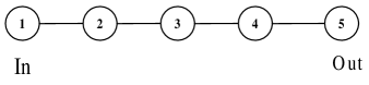
Figure 1: Five qudit cluster used in realization of $X^{\alpha}(\{m\})$ and $Z^{\alpha}(\{m\})$. A circle represents one qudit, number $n$ in the circle means the $n$-th qudit, $in$ or $out$ denote the input or output part of the cluster, and two qudits which are connected by a line is neighbors.

The corresponding cluster state is defined by the following system of equations:

$$X_{1}^{\dagger}Z_{2}|\phi\rangle_{\mathcal{C}} = |\phi\rangle_{\mathcal{C}},$$ (77)

$$Z_{1}X_{2}^{\dagger}Z_{3}|\phi\rangle_{\mathcal{C}} = |\phi\rangle_{\mathcal{C}},$$ (78)

$$Z_{2}X_{3}^{\dagger}Z_{4}|\phi\rangle_{\mathcal{C}} = |\phi\rangle_{\mathcal{C}},$$ (79)

$$Z_{3}X_{4}^{\dagger}Z_{5}|\phi\rangle_{\mathcal{C}} = |\phi\rangle_{\mathcal{C}},$$ (80)

$$Z_{4}X_{5}^{\dagger}|\phi\rangle_{\mathcal{C}} = |\phi\rangle_{\mathcal{C}}.$$ (81)

It follows from Eqs. (77-81) that

$$X_{1}X_{3}^{\dagger}X_{5}|\phi\rangle_{\mathcal{C}} = |\phi\rangle_{\mathcal{C}},$$ (82)

$$Z_{1}^{\dagger}X_{2}X_{4}^{\dagger}Z_{5}|\phi\rangle_{\mathcal{C}} = |\phi\rangle_{\mathcal{C}}.$$ (83)

Form Eq. (81), we obtain

$$Z_{4}^{\dagger\alpha}(\{m\})X_{5}^{\alpha}(\{m\})|\phi\rangle_{\mathcal{C}}=|\phi\rangle_{\mathcal{C}}.$$ (84)

Here we emphasizes that when we obtain the above equation, we have used the following condition On $\{m\}$. If $n_{4}+n_{5}=0\;(Mod(d))$, then

$$n_{4}+m_{n_{4}}+n_{5}+m_{n_{5}}=0,\;(n_{4},n_{5}\in Z_{d}).$$ (85)

From the above four equations, we have

$$X_{1}X_{3}^{\dagger}\left(X_{5}^{\alpha}\left(\{m\}\right)X_{5}X_{5}^{\dagger\alpha}\left(\{m\}\right)\right)|\phi\rangle_{\mathcal{C}} = |\phi\rangle_{\mathcal{C}},$$ (86)

$$Z_{1}^{\dagger}X_{2}\left(Z_{4}^{\dagger\alpha}(\{m\})X_{4}^{\dagger}Z_{4}^{\alpha}(\{m\})\right)\left(X_{5}^{\alpha}(\{m\})Z_{5}X_{5}^{\dagger\alpha}(\{m\})\right)|\phi\rangle_{\mathcal{C}} = |\phi\rangle_{\mathcal{C}}.$$ (87)

For a measurement pattern $\{X_{2},\,X_{3}^{\dagger},\,Z_{4}^{\dagger\alpha}(\{m\})X_{4}^{\dagger}Z_{4}^{\alpha}(\{m\})\}$, Theorem 2 concludes that the simulated unitary transformation is $X_{5}^{\alpha}(\{m\})U_{\Sigma}$, where

$$U_{\Sigma}=Z_{5}^{-s_{1}-s_{3}}X_{5}^{s_{2}+s_{4}}.$$

Because $U_{\Sigma}$ depends on the measurement results and can not be moved to the front of $X_{5}^{\alpha}(\{m\})$ trivially, different measurement results lead to different unitary transformations. In order to realize unique gate $X_{5}^{\alpha}(\{m\})$, we complete the measurement in two steps: In the first step, we measure $\{X_{1},X_{2},X_{3}^{\dagger}\}$. Then, when the obtained values are $s_{1}$ , $\lambda_{x}\,(=s_{3})$ and $s_{2}$, the byproduct operator reads $U_{\Sigma}=Z^{-s_{3}-s_{1}}X^{\lambda_{z}}$. At this time, $\lambda_{z}$ is still unknown since it depends on the measured result $s_{4}$. However, notice that $Z_{5}^{-s_{3}-s_{1}}X_{5}^{\alpha}(\{m\})Z_{5}^{s_{3}+s_{3}}$ is diagonal in the $X$ representation, we have

$$Z_{5}^{-s_{3}-s_{1}}X_{5}^{\alpha}(\{m\})Z_{5}^{s_{3}+s_{1}}=\prod_{\{m\}}X_{5}^{\alpha^{s_{1}s_{3}}_{\{m\}}}(\{m\}).$$ (88)

From Eq. (88), we can obtain $d$ equations of $\{\alpha^{s_{1}s_{3}}_{\{m\}}\}$, which determine the values of $\{\alpha^{s_{1}s_{3}}_{\{m\}}\}$.

Now we make a new choice depending on the known measurement results. Also from Eqs. (77-81), we obtain the following equation instead of Eq. (87)

$$Z_{1}^{\dagger}X_{2}\left(\prod_{\{m\}}Z_{4}^{\dagger\alpha^{s_{1}s_{3}}_{\{m\}}}(\{m\})X_{4}^{\dagger}\prod_{\{m\}}Z_{4}^{\alpha^{s_{1}s_{3}}_{\{m\}}}(\{m\})\right)$$

$$\left(\prod_{\{m\}}X_{5}^{\alpha^{s_{1}s_{3}}_{\{m\}}}(\{m\})Z_{5}\prod_{\{m\}}X_{5}^{\dagger\alpha^{s_{1}s_{3}}_{\{m\}}}(\{m\})\right)|\phi\rangle_{\mathcal{C}}=|\phi\rangle_{\mathcal{C}}.$$ (89)

Measuring the fourth qudit in the base

$$\prod_{\{m\}}Z_{4}^{\dagger\alpha^{s_{1}s_{3}}_{\{m\}}}(\{m\})X_{4}^{\dagger}\prod_{\{m\}}Z_{4}^{\alpha^{s_{1}s_{3}}_{\{m\}}}(\{m\}),$$

we obtain the value $s_{4}$ and therefore $\lambda_{z}=s_{2}+s_{4}$. According to Theorem 2, we obtain the final operation

$$UU_{\Sigma}=Z_{5}^{-s_{3}-s_{1}}X_{5}^{s_{2}+s_{4}}X_{5}^{\alpha}(\{m\}).$$ (90)

Finally, by measuring $Z_{5}$ we obtain the correct result

$$s=s_{5}+s_{2}+s_{4}.$$ (91)

The above equation does not mean that the final result depends only on the measurements to the second, fourth, and fifth qudit, because different values of $s_{1}$ and $s_{3}$ correspond to different measurement on the fourth qudit.

Based on the same cluster, we can also implement the single qudit rotation $Z^{\alpha}(\{m\})$. Similarly, we first measure $\{X_{1},X_{2},x^{\dagger}_{4}\}$; Then from Eqs. (77-81), we obtain

$$X_{1}\left(\prod_{m}Z_{3}^{\alpha^{s_{2}s_{4}}_{\{m\}}}(\{m\})X_{3}^{\dagger}\prod_{m}Z_{3}^{\dagger\alpha^{s_{2}s_{4}}_{\{m\}}}(\{m\})\right)$$

$$\left(\prod_{m}Z_{5}^{\alpha^{s_{2}s_{4}}_{\{m\}}}(\{m\})X_{5}\prod_{m}Z_{5}^{\dagger\alpha^{s_{2}s_{4}}_{\{m\}}}(\{m\})\right)|\phi\rangle_{\mathcal{C}} = |\phi\rangle_{\mathcal{C}},$$ (92)

$$Z_{1}^{\dagger}X_{2}X_{4}^{\dagger}Z_{5}|\phi\rangle_{\mathcal{C}} = |\phi\rangle_{\mathcal{C}}.$$ (93)

where $\{\alpha^{s_{2}s_{4}}_{\{m\}}\}$ is determined by

$$X_{5}^{s_{2}+s_{4}}Z_{5}^{\alpha}({\{m\}})X_{5}^{-s_{2}-s_{4}}=\prod_{\{m\}}Z_{5}^{\alpha_{\{m\}}^{s_{2}s_{4}}}({\{m\}}).$$ (94)

At the same time we make another measurement on

$$\prod_{m}Z_{3}^{\alpha^{s_{2}s_{4}}_{\{m\}}}(\{m\})X_{3}^{\dagger}\prod_{m}Z_{3}^{\dagger\alpha^{s_{2}s_{4}}_{\{m\}}}(\{m\}).$$

According to theorem 2, we conclude that the simulated unitary transformation indeed is

$$Z^{-s_{3}-s_{1}}X^{s_{2}+s_{4}}Z_{5}^{\alpha}({\{m\}}).$$

The correct result and the measurement values are also related by Eq. (91).

V.1.2 Realizations of single qudit elements in Clifford group

As implied in Eq. (76), we only need to realize the single qudit elements in the Clifford group. It is easy to show that not all elements in the Clifford group are required. In fact, we only need do the elements defined as

$$U^{mn}Z{U^{mn}}^{\dagger}=\bar{Z},$$ (95)

where

$$\bar{Z}=q_{d}^{-\frac{d-1}{2}mn}Z^{m}X^{n},$$ (96)

with

$$(m,n)=1.$$ (97)

We will show that we can do all the above Clifford unitary transformations through a series of four basic types of unitary transformations. The first is defined as

$$U^{1n}Z{{U^{1n}}^{\dagger}} = q_{d}^{-\frac{d-1}{2}n}ZX^{n},$$ (98)

$$U^{1n}X{{U^{1n}}^{\dagger}} = X;$$ (99)

The second is defined as

$$U^{n1}Z{{U^{n1}}^{\dagger}} = q_{d}^{-\frac{d-1}{2}n}Z^{n}X,$$ (100)

$$U^{n1}X{{U^{n1}}^{\dagger}} = Z^{\dagger};$$ (101)

The third is defined as

$$VZ{{V}^{\dagger}} = q_{d}^{-\frac{d-1}{2}}ZX,$$ (102)

$$VX{{V}^{\dagger}} = X;$$ (103)

The last is defined as

$$WZ{{W}^{\dagger}} = Z,$$ (104)

$$WX{{W}^{\dagger}} = q_{d}^{-\frac{d-1}{2}}ZX.$$ (105)

Theorem 3

For any unitary transformation $U^{mn}$ partially defined by Eq. (95), it can be factorized into a product of a series of the above four basic unitary transformations.

Proof. Let us prove it by induction. We denote $N_{d}\equiv\{1,2,\cdots,d\}$. When $m=1$ or $n=1$, it is the first or the second types of unitary transformations. Let us suppose the above theorem is valid at $m\in N_{d}$ or $n\in N_{d}$, i.e., we can do

$$U^{mn}\qquad(m\;\mbox{or}\;n\in N_{d},\,(m,n)=1).$$ (106)

For arbitrary positive integer $n$ that is relatively prime to $d+1$, there exists

$$n=i(d+1)+n^{\prime},\quad(i\in Z_{\infty},\,n^{\prime}\in N_{d}).$$ (107)

Obviously,

$$n^{\prime}\in N_{d},\,(d+1,n^{\prime})=1.$$ (108)

According to the assumption, we can do $U^{(d+1)n^{\prime}}$. Then let $V$ operate $i$ times,

$$V^{i}U^{(d+1)n^{\prime}}{V^{\dagger}}^{i}=U^{(d+1)n}.$$ (109)

According to the assumption, we can also do $U^{n^{\prime}(d+1)}$. Then let $W$ operate $i$ times,

$$W^{i}U^{n^{\prime}(d+1)}{W^{\dagger}}^{i}=U^{n(d+1)}.$$ (110)

Therefore the theorem is valid for $m\;\mbox{or}\;n\in N_{d+1}$. This completes the proof. $\Box$

Now we come to constructing the four basic unitary transformations. We will prove that the first (including the third) and the fourth can be realized on the five qudit cluster as Fig. 1. According to Eqs. (77-81), we have

$$X_{1}X_{3}^{\dagger}X_{5}|\phi\rangle_{\mathcal{C}} = |\phi\rangle_{\mathcal{C}},$$ (111)

$$Z_{1}^{\dagger}X_{2}({Z_{4}}^{n}X_{4})^{\dagger}Z_{5}{X_{5}}^{n}|\phi\rangle_{\mathcal{C}} = |\phi\rangle_{\mathcal{C}}.$$ (112)

According to theorem 2, when the measurement pattern is $\{X_{2},\,X_{3}^{\dagger},\,({q_{d}}^{-\frac{d-1}{2}n}{Z_{4}}^{n}X_{4})^{\dagger}\}$, the corresponding unitary transformation is

$${q_{d}}^{\frac{d-1}{2}(s_{1}+s_{3})n}Z^{-s_{1}-s_{3}}X^{s_{2}+s_{4}-n(s_{1}+s_{3})}U^{1n}.$$ (113)

Also from Eqs. (77-81), we obtain

$$X_{1}Z_{3}X_{3}^{\dagger}X_{4}^{\dagger}Z_{5}X_{5}|\phi\rangle_{\mathcal{C}} = |\phi\rangle_{\mathcal{C}},$$ (114)

$$Z_{1}^{\dagger}X_{2}X_{4}^{\dagger}Z_{5}|\phi\rangle_{\mathcal{C}} = |\phi\rangle_{\mathcal{C}}.$$ (115)

According to theorem 2, when the measurement pattern is $\{X_{2},\,{q_{d}}^{\frac{d-1}{2}n}Z_{3}X_{3}^{\dagger},\,X_{4}^{\dagger}\}$, the corresponding unitary transformation is

$${q_{d}}^{\frac{d-1}{2}(s_{2}+s_{4})}Z^{s_{2}-s_{1}-s_{3}}X^{s_{2}+s_{4}}W.$$ (116)

To realize the unitary transformation $U^{n1}$, we need a cluster composed of six qudits as Fig. 2.

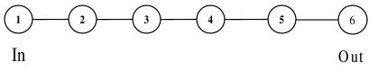
Figure 2: Six qudit cluster used in realization of $U^{n1}$. Meanings of the symbols in this Figure are the same as Fig. 1.

The cluster state is defined by the following system of equations

$$X_{1}^{\dagger}Z_{2}|\phi_{\mathcal{C}}\rangle = |\phi\rangle_{\mathcal{C}},$$ (117)

$$Z_{1}X_{2}^{\dagger}Z_{3}|\phi\rangle_{\mathcal{C}} = |\phi\rangle_{\mathcal{C}},$$ (118)

$$Z_{2}X_{3}^{\dagger}Z_{4}|\phi\rangle_{\mathcal{C}} = |\phi\rangle_{\mathcal{C}},$$ (119)

$$Z_{3}X_{4}^{\dagger}Z_{5}|\phi\rangle_{\mathcal{C}} = |\phi\rangle_{\mathcal{C}},$$ (120)

$$Z_{4}X_{5}^{\dagger}Z_{6}|\phi\rangle_{\mathcal{C}} = |\phi\rangle_{\mathcal{C}},$$ (121)

$$Z_{5}X_{6}^{\dagger}|\phi\rangle_{\mathcal{C}} = |\phi\rangle_{\mathcal{C}}.$$ (122)

It follows from the above equations that

$$X_{1}X_{3}^{\dagger}X_{5}Z_{6}^{\dagger}|\phi\rangle_{\mathcal{C}} = |\phi\rangle_{\mathcal{C}},$$ (123)

$$Z_{1}^{\dagger}X_{2}{Z_{4}}^{n}X_{4}^{\dagger}{X_{5}^{\dagger}}^{n}{Z_{6}}^{n}X_{6}|\phi\rangle_{\mathcal{C}} = |\phi\rangle_{\mathcal{C}}.$$ (124)

When the measurement pattern is $\{X_{2},\,X_{3}^{\dagger},\,{q_{d}}^{\frac{d-1}{2}n}{Z_{4}}^{n}X_{4}^{\dagger},\,X_{5}\}$, the corresponding unitary transformation is

$${q_{d}}^{(s_{1}+s_{3})(s_{2}+s_{4}-ns_{5}+\frac{d-1}{2}n)}Z^{n(s_{5}-s_{1}-s_{3})-s_{2}-s_{4}}X^{-s_{1}-s_{3}}U^{n1}.$$ (125)

V.2
Realization of an imprimitive two qudit gate

Now we come to the construction for simulating two qudit operations.

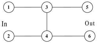
Figure 3: Six qudit cluster used in realization of an imprimitive two qudit gate $T$. Meanings of the symbols in this Figure are the same as Fig. 1.

The cluster composed of six qudits as Fig. 3 is considered with the following system of equations

$$X_{1}^{\dagger}Z_{3}|\phi_{C}\rangle = |\phi\rangle_{\mathcal{C}},$$ (126)

$$X_{2}^{\dagger}Z_{4}|\phi\rangle_{\mathcal{C}} = |\phi\rangle_{\mathcal{C}},$$ (127)

$$Z_{1}X_{3}^{\dagger}Z_{4}Z_{5}|\phi\rangle_{\mathcal{C}} = |\phi\rangle_{\mathcal{C}},$$ (128)

$$Z_{2}Z_{3}X_{4}^{\dagger}Z_{6}|\phi\rangle_{\mathcal{C}} = |\phi\rangle_{\mathcal{C}},$$ (129)

$$Z_{3}X_{5}^{\dagger}|\phi\rangle_{\mathcal{C}} = |\phi\rangle_{\mathcal{C}},$$ (130)

$$Z_{4}X_{6}^{\dagger}|\phi\rangle_{\mathcal{C}} = |\phi\rangle_{\mathcal{C}}.$$ (131)

It follows from the above equations that

$$X_{1}X_{5}^{\dagger}|\phi\rangle_{\mathcal{C}} = |\phi\rangle_{\mathcal{C}},$$ (132)

$$X_{2}X_{6}^{\dagger}|\phi\rangle_{\mathcal{C}} = |\phi\rangle_{\mathcal{C}},$$ (133)

$$Z_{1}^{\dagger}X_{3}Z_{5}^{\dagger}X_{6}^{\dagger}|\phi\rangle_{\mathcal{C}} = |\phi\rangle_{\mathcal{C}},$$ (134)

$$Z_{2}^{\dagger}X_{4}Z_{6}^{\dagger}X_{5}^{\dagger}|\phi\rangle_{\mathcal{C}} = |\phi\rangle_{\mathcal{C}}.$$ (135)

By measuring the system according to the measurement pattern $\{X_{1}X_{2}X_{3}X_{4}Z_{5}Z_{6}\}$, the simulated two qudit gate $T$ satisfies, and is also defined by

$$TX_{5}T^{\dagger} = X_{5}^{\dagger},$$ (136)

$$TX_{6}T^{\dagger} = X_{6}^{\dagger},$$ (137)

$$TZ_{5}T^{\dagger} = Z_{5}^{\dagger}X_{6}^{\dagger},$$ (138)

$$TZ_{6}T^{\dagger} = Z_{6}^{\dagger}X_{5}^{\dagger}.$$ (139)

According to Theorem 2, the above measurement pattern realize the following unitary gate

$$TZ_{5}^{-s_{1}}X_{5}^{s_{3}}Z_{6}^{-s_{2}}X_{6}^{s_{4}}={q_{d}}^{s_{1}s_{2}}Z_{5}^{s_{1}}X_{5}^{s_{2}-s_{3}}Z_{6}^{s_{2}}X_{6}^{s_{1}-s_{4}}T.$$ (140)

The next task is to prove that $T$ is an imprimitive two qudit operation. Ref. Bry tells us that a two gate $V$ is primitive if and only if $V=S_{1}\otimes S_{2}$ or $V=(S_{1}\otimes S_{2})P$. Here, $S_{1}$ and $S_{2}$ are different single qudit operators, $P$ is the interchanging operator obeying $P|x\rangle\otimes|y\rangle=|y\rangle\otimes|x\rangle$. Based on this fact, we can easily conclude that a primitive operator always maps a single qudit operator to another single qudit operator. Obviously, the above two qudit operator $T$ is imprimitive. Another way to prove it is to evaluate the unitary transformation directly. Then we can find that it maps all $Z\otimes Z-$ bases to the maximum entangle states.

As demonstrated in this section, any single qudit unitary gate and one imprimitive two qudit gate can be realized on qudit clusters. Therefore, the measurement based quantum computing on qudit clusters is universal.

VI Conclusions

We have introduced the concept of qudit cluster state in terms of finite dimensional representations of QPA. Based on these qudit cluster states, we have built all the elements of qudit clusters needed for implementation of universal measurement-based quantum computations. With generalizations of cluster states and measurement patterns, most of the results in qubit cluster can work well for qudit clusters in parallel ways. We also show that there still exists the celebrated theorem guaranteeing the availability of qudit cluster states to quantum computations. To prove the universality of this quantum computation, we show that we can implement all single qudit unitary transformations and one imprimitive two qudit gate on specific qudit clusters. In addition, we propose to build a one-way universal quantum computer with qudit cluster states practically since the high dimensional “Ising”model can be used to generate such cluster state dynamically.

References

• (1) M. A. Nielsen and I. S. Chuang, Quantm computation and quantum information, Cambridge University Press (2000).
• (2) H. J. Briegel and R. Raussendorf, Phys. Rev. Lett. 86, 910 (2001).
• (3) R. Raussendorf and H. J. Briegel, Phys. Rev. Lett. 86, 5188 (2001).
• (4) R. Raussendorf, D. E. Browne, and H. J. Briegel, quant-ph/0301052 (2003).
• (5) L. M. Duan, E. Demler, and M. D. Lukin, cond-mat/0201564 (2002).
• (6) C. P. Sun, in “Quantum Group and Quantum Integrable Systems”, ed by M. L. Ge, World Scientific, 1992, p.133; M. L. Ge, X. F. Liu, C. P. Sun, J. Phys A-Math Gen 25 (10): 2907, (1992).
• (7) S. D. Bartlett, H. de Guise, and B. C. Sanders, Phys. Rev. A65, 052316 (2002).
• (8) B. C. Sanders, S. D. Barlett, and H. de Guise, quant-ph/0208008(2002).
• (9) J. Jamil, X. G. Wang, and B. C. Sanders, quant-ph/0211185 (2002).
• (10) D. Gottemann, A. Kitaev and J. Preskill, Phys. Rev. A65, 044303 (2002).
• (11) J. Patera and H. Zassenhaus, J. Math. Phys. 29, 665 (1988).
• (12) E. Knill, quant-ph/9608048 (1996).
• (13) H. Weyl, Theory of groups and quantum mechanics, New York: E. P. Dutton Co., (1932).
• (14) J. Schwinger, Proceedings of the National Academy of Sciences, 46 (4), 570 (1960).
• (15) R. R. Puri, Mathematical methods of quantum optics, Springer press (2001).
• (16) J. L. Brylinski and R. Brylinski, quant-ph/0108062 (2001).
• (17) M. Blume, V. J. Emery, and R. B. Griffiths, Phys. Rev. A4, 1071 (1971).
• (18) J. Sivardiere and M. Blume, Phys. Rev. B5, 1126 (1972).
• (19) J. Kwo et al., Phys. Rev. Lett. 55, 1402 (1985).
• (20) C. F.Majkrzak et al., Phys. Rev. Lett. 56, 2700 (1986).
• (21) J. J. Krebs, P. Lubirtz, A. Chaiken, and G. A. Prinz, Phys. Rev. Lett. 63, 1645 (1989).
• (22) R. E. Camiey, J. Kwo, M. Hong, and C. L. Chien, Phys. Rev. Lett. 64, 2703 (1990).
• (23) N. Sh. Izmailian, arXiv:hep-th/9603080.
• (24) A. Mattoni, M. Bagagiolo, and A. Saber1, Chinese Journal of Physics 40, 3, 2002.
• (25) L. L. Hinchey and D. L. Mills, Phys. Rev. B33, 3329 (1986).
• (26) B. D. Qu, W. L. Zhong, P. L. Zhang, Phys. Lett. A189, 419 (1994).
• (27) F. Fisman, F. Schwabl, and D. Schwenk, Phys. Lett. A121, 192 (1987).
• (28) J. Gritz-Saaverda, F. Aguilra-Grania, and J. L. Moran-Lopez, Solid State Commun. 82, 5891 (1992).
• (29) H. K. Sy and M. H. Ow, J. Phys. Condens. Matter, 4, 5891 (1992).
• (30) A. Saber, A. Ainane, M. Saber, I. Essaoudi, F. Dujardin, and B. St eb e, Phys. Rev. B60, 4149 (1999).