Maximizing the Hilbert space for a finite number of distinguishable quantum states.

Abstract

We consider a quantum system with a finite number of distinguishable quantum states, which may be partitioned freely by a number of quantum particles, assumed to be maximally entangled. We show that if we partition the system into a number of qudits, then the Hilbert space dimension is maximized when each quantum particle is allowed to represent a qudit of order $e$. We demonstrate that the dimensionality of an entangled system, constrained by the total number quantum states, partitioned so as to maximize the number of qutrits will always exceed the dimensionality of other qudit partitioning. We then show that if we relax the requirement of partitioning the system into qudits, but instead let the particles exist in any given state, that the Hilbert space dimension is greatly increased.

Quantum computation bib:NielsenBook has, in remarkably short time, become one of the most interesting fields in applied quantum physics today. There are numerous suggestions for implementing quantum computers. One common feature of all scalable quantum computers, is their use of entangled particles bib:Blume-Kohout2002 .

Most quantum computer proposals focus on qubits (quantum bits) as the fundamental element of computing. These are two state quantum systems that can be entangled. Further work has begun to examine the possibility of performing computations with qudits (quantum digits) bib:QuditRef . Qudits are an extension of qubits, that are systems with any (integer) number of states greater than 1. The qubit is therefore the two-state qudit, and the qutrit is the three-state qudit. For convenience we will refer to the $x$-state qudit as an x-qudit.

Investigations into qudits have shown many significant results. Entanglement between two qutrits was first discussed by Caves and Milburn bib:QutritEntanglement . Bell inequalities for systems of qudits are more strongly violated than analogous systems of qubits bib:BellViolation , and recent experiments have shown entanglement of two qutrits, realized using the orbital angular momentum as the quantum state bib:VaziriPRL2002 . A quantum-communication protocol using qutrits has also been proposed bib:QutritCommunication . Universal quantum gates and gate fidelity have been studied for qudit systems bib:QuditGates , a readout method based on quantum state tomography has been proposed bib:QST and the extension of infinite-dimensional qudits to continuous-variable quantum computation has also been made bib:SandersPreprint2002 .

The Hilbert-space dimension of a quantum computer has been identified as the primary resource for any physical realization of such a device bib:Blume-Kohout2002 . To that end it is necessary to consider how best to maximize the Hilbert-space dimension for a given quantum computer geometry. It is obvious that for a given number of particles, the dimensionality of the Hilbert space, ${\cal D}$, will be increased by increasing the dimensionality of the particles, although it is not, in general, trivial to increase the dimensionality of the fundamental particles being used for the computation; nor is the added complexity involved necessarily favorable. However there are proposals for quantum computing which involve a number of quantum particles having available a finite number of distinguishable quantum states. Examples include the charge-qubit scheme bib:EkertRMP1996 ; bib:Hollenberg , superconducting Cooper-pair boxes bib:CooperPairBox , quantum computing based on photons in interferometers joined by lossless nonlinear optical elements bib:QNLO and the linear optics implementation bib:KLM . In all these proposals the fundamental quantum particles (electrons, Cooper-pairs or photons) may be in a finite number of distinguishable quantum states (positions, interferometer arms). These quantum states are grouped together and we term such groupings quantum elements. For qudits we have one particle per quantum element, which can be in a superposition of all states within the element. Ideally every particle will be entangled with every other particle.

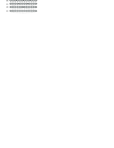
Figure 1: Possible groupings of a linear array of 12 distinguishable quantum sites into various quantum qudit partitions. Qudit groupings are shown schematically as dashed ovals, and open circles are quantum sites. (a) Partitioning into six qubits, (b) partitioning into four qutrits, (c) partitioning into three 4-qudits, (d) partitioning into two 6-qudits, (e) partitioning into one 12-qudit.

For concreteness, we will consider the charge scheme of Hollenberg et al. bib:Hollenberg , although the generalization to other schemes is straightforward. Without examining issues related to operational complexity or physical architecture we will show ways in which to optimize the Hilbert-space dimensionality for a system where the number of accessible quantum states is unchanging, although the logical groupings of those states into quantum elements, and the number of particles shared between those states is varied.

Consider a linear array of $N$ donor impurities, with controllable tunnelling probabilities and individual energy levels. If we partition the space into $x$-qudits, as shown in Fig. 1 for $x=2,3,4$, then we must introduce $N/x$ electrons. The dimension of the Hilbert space obtained by maximally entangling these N/x electrons is therefore:

$${\cal D}_{x}=x^{N/x}.$$ (1)

Simply differentiating Eq. 1 allows us to determine the value of $x$ which maximizes ${\cal D}$ for a given $N$

$$\frac{d{\cal D}}{dx}=-Nx^{\frac{N}{x}-2}(\ln x-1)=0,$$

$$\Rightarrow x=e.$$

As each particle needs to have an integer number of levels, we note that for identical qudits, the dimensionality is optimized for qutrits. The Hilbert-space dimensionality for qutrits over qubits will be larger by a factor ${\cal D}_{3}/{\cal D}_{2}=\exp\left[N\left(\ln 3/3-\ln 2/2\right)\right]$.

In Fig. 2 we show the Hilbert-space dimensionality of a twelve-state system as a function of the size of each quantum element. Each different case is explained through the text. The $+$ symbols in Fig. 2 show the dimensionality associated with qudit arrangements. As expected, the dimensionality is maximized by a qudit size of 3 (note that we are only showing integer qudit sizes). For the system with 12 quantum states, ${\cal D}_{2}=64$ whereas ${\cal D}_{3}=81$.

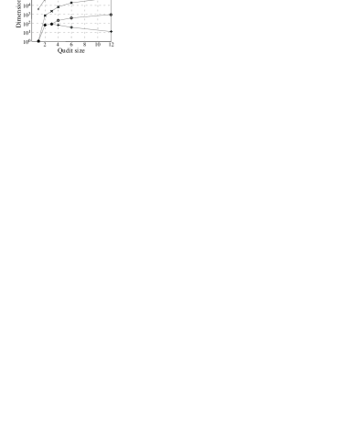
Figure 2: Hilbert space dimensionality for various geometries as a function of qudit size for $N$ distinguishable quantum states. $+$ corresponds to equipartitioning into qudits, $\circ$ to a $Q_{x}(x/2,1)$ partition, $\times$ to a $Q_{x}(x,2)$ partition and $\ast$ to spin referenced systems. Note that the dimensionalities are only valid when $N/x$ is an integer greater than one, i.e. for $x=2,3,4,6,12$. The lines are merely guides for the eye.

Conceivably, it may be possible to realize a quantum computer which uses a mixture of qubits and qutrits so as to optimize the total dimensionality of the Hilbert space, as recently discussed by Daboul et al. bib:DaboulPreprint2002 . For instance, suppose we partition the space into $y_{2}$ qubits and $y_{3}$ qutrits such that $2y_{2}+3y_{3}=N^{\prime}$ where $N^{\prime}\lesssim N$. One might guess that the dimensionality of the Hilbert space would be increased by mixing qubits and qutrits such that the average dimensionality of the system $(2y_{2}+3y_{3})/(y_{2}+y_{3})$ is closer to the optimal value $e$. However, this is not the case. To see why, note that the dimensionality of the Hilbert space of a system partitioned as suggested is given by $2^{y_{2}}3^{y_{3}}=2^{(N^{\prime}-3y_{3})/2}3^{y_{3}}$. With ${\cal D}_{e}=exp(N^{\prime}/e)$ this leads to

$${\cal D}/{\cal D}_{e}=\exp(my_{3}+b),$$

where $m=\ln(3)-\frac{3}{2}\ln(2)>0$ and $b=(\frac{\ln(2)}{2}-e^{-1})N^{\prime}$. Note that $\exp(my_{3}+b)=1$ if $y_{3}=-b/m\approx 0.36N^{\prime}$. Since $y_{3}\leq N^{\prime}/3$ on physical grounds, this implies $my_{3}+b<0$, i.e., the exponential is always less than one. Furthermore, since $m>0$, the value of the exponential increases with the number of qutrits $y_{3}$. Thus, the dimensionality of the Hilbert space is optimized if we partition the system into the largest available number of qutrits, except where adding a single qubit would more efficiently use all of the available quantum states.

Allowing the number of particles to vary within each quantum element changes the system dimensionality and generalizes the qudit scheme. We consider quantum elements which are groupings of $x$ quantum states (modes), with $k$ particles per quantum element and at most $l$ particles per state. Such an arrangement is shown schematically in Fig. 3. We term these structures $(k,l)$ packing x-qudits and use the shorthand notation $Q_{x}(k,l)$, writing the dimensionality of these structures as $\dim[Q_{x}(k,l)]$. In essence, this approach reverses the work of Abrams and Lloyd bib:AbramsPRL1997 where an algorithm for efficient simulation of many-body Fermi systems on a quantum computer was presented, by proposing a many-body system as a quantum computer in its own right, and is in keeping with Bravyi and Kitaev’s work on fermionic quantum computation bib:BravyiPreprint2000 . Blume-Kohout et al. bib:Blume-Kohout2002 calculated the dimensionality of Fermionic and Bosonic systems, which in our notation would correspond to $Q_{x}(k,1)$ and $Q_{x}(k,k)$ respectively. We note that analysis of two electrons in a polygonal dot ($Q_{x}(2,1)$), has been performed by Creffield et al. bib:Creffield . Creffield and Platero studied two electrons in a square dot bib:CreffieldPRB2002 , considering the possibility of double occupancy ($Q_{4}(2,2)$). This system (without double occupancy) has also been proposed as a scalable quantum element by Jefferson et al. bib:JeffersonPRA2002 ($Q_{4}(2,1)$).

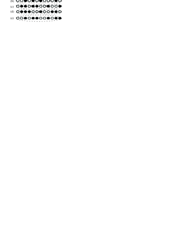
Figure 3: Possible groupings of a linear array of 12 distinguishable quantum sites into various $Q_{x}(k,1)$ partitions. The x-qudit groupings are shown schematically as dashed ovals, open circles are quantum sites and filled circles correspond to (randomly chosen) filled sites. (a) six $Q_{2}(1,1)$ partitions, (b) four $Q_{3}(1,1)$ partitions, (c) three $Q_{4}(2,1)$ partitions, (d) two $Q_{6}(3,1)$ partitions, (e) one $Q_{12}(6,1)$ partition.

We first consider the case that there can be no more than one particle per quantum state, but the number of particles per element is chosen to maximise the Hilbert-space dimensionality, i.e. the $Q_{x}(k,1)$ partition, or Fermionic system. In order to maximize the total Hilbert-space dimensionality, it is clear that the number of particles per quantum element must be equal to the number of sites divided by 2, i.e. $k=x/2$ for $x$ even, or $k=(x\pm 1)/2$ for $x$ odd, where the $\pm$ is due to symmetry between particles and holes. The total dimensionality for a system with $N$ sites, partitioned into $N/x$ elements will therefore be (assuming $x$ even and $N/x$ an integer)

$${\cal D}=\{\dim[Q_{x}(x/2,1)]\}^{N/x}={x\choose{x/2}}^{N/x}.$$

where ${n\choose m}$ is the number of possible identifiably different permutations of $n$ elements of two different types, $m$ of which are of type 1 (eg. particles) and $n-m$ of which are of type 2 (eg. holes or empty sites). The Hilbert-space dimensionality showing this form of partitioning is represented by the open circles $\circ$ in Fig. 2. The total dimensionality, $\dim[Q_{x}(x/2,1)]$, is clearly maximized when $x=N$, which corresponds to the case that all particles are allowed to roam freely in the lattice, which is the case of local fermionic modes discussed by Bravyi and Kitaev bib:BravyiPreprint2000 and is scalable, as discussed by Blume-Kohout bib:Blume-Kohout2002 . In a twelve state configuration, for example, Fig. 3(e) shows the configuration which maximizes the dimensionality of the Hilbert-space, with $\dim[Q_{12}(6,1)]=924$, an order of magnitude larger than case of qutrits. Despite this maximization, it is important to realize that there may well be advantages to partitioning into smaller subspaces (i.e. $x<N$) - for example it is not possible to do error correction without some degree of redundancy in coding.

The next obvious extension is to allow the maximum number of particles per site to increase to two. This could physically correspond to an electron based quantum computer, where the charging energy of two particles per dot can be overcome bib:CreffieldPRB2002 . In this case the dimensionality of the system will be

$${\cal D}=\{\dim[Q_{x}(k,2)]\}^{N/x}=\left[\sum_{j_{2}=0}^{k/2}{x\choose{j_{2}}}{{x-j_{2}}\choose{k-2j_{2}}}\right]^{N/x},$$

where $j_{2}$ indexes the number of sites with two electrons per site and is allowed to range from $0$ to $N/2$ for $x$ even, or $0$ to $(N-1)/2$ for $x$ odd. It is straightforward to show that the dimensionality of each partition is maximized when $k=x$, i.e. the number of particles per element is equal to the number of sites per element. The dimensionality in this case is shown by the crosses, $\times$, in Fig. 2, which is significantly larger than the case where at most one particle is allowed per site.

Another alternative is where we have an extra quantum number (for example spin), which would double the number of accessible quantum states. In this case the system returns to the standard Fermionic case and the dimensionality becomes simply

$${\cal D}={{2x}\choose k}^{N/x}.$$

This dimensionality is shown by the asterisks, $\ast$, in Fig. 2 which represents the largest dimensionality of all the cases under consideration.

In general, we note that if we allow the number of particles per site to be at most $z$, then the total Hilbert-space dimensionality is

$$\{\dim[Q_{x}(k,z)]\}^{N/x}=\left[\sum_{j_{z}=0}^{x/z}{x\choose{j_{z}}}\sum_{j_{z-1}=0}^{(k-zj_{z})/(z-1)}{{x-j_{z}}\choose{j_{z-1}}}\cdots\sum_{j_{2}=0}^{(k-\sum_{r=3}^{z}rj_{r})/2}{{x-\sum_{r=3}^{z}j_{r}}\choose{j_{2}}}{{x-\sum_{r=2}^{z}j_{r}}\choose{k-\sum_{r=2}^{z}rj_{r}}}\right]^{N/x}.$$

Note that if there is no restriction on the number of particles per site we retrieve the Bosonic case. We would then be looking to extend familiar bosonic quantum computing schemes to the multiple-particle limit, for example linear optical bib:KLM , nonlinear optical bib:QNLO or superconducting bib:CooperPairBox quantum computing schemes. The dimensionality is considerably simplified and is bib:Blume-Kohout2002 ; bib:MayerText

$$\dim[Q_{x}(k,k)]={{x+k-1}\choose{x-1}}.$$

This dimensionality can greatly exceed the fermionic case, for the same number of accessible quantum states, for a large enough number of particles. Furthermore this dimensionality monotonically increases with increasing particle number. This suggests that a quantum computing architecture based around bosons may be easier to upgrade than any other architecture.

We note in closing that there is far more to quantum computers than optimizing the Hilbert space dimension. Here we have not entered into issues of operational complexity, which will be specific to particular architectures, as well as decoherence which is expected to differ substantially between implementations. However, comparing qudit implementations, a system comprising qubits alone will maximize the amount of information that can be obtained in a single measurement step. This is because an optimum measurement would be to measure the state of every quantum particle. For qubits, that would yield $N/2$ values; for qutrits, it would only yield $N/3$ values. As a rough measure, we may say that to equalize the amount of information gained about the state of the computer, we would need to perform $(N/2)/(N/3)=1.5$ times as many measurements on a qutrit-based quantum computer as a qubit-based quantum computer. The dimensionality of the qutrit Hilbert space exceeds that of the qubit Hilbert space by $1.5$ when

$$\exp\left[N\left(\frac{\ln 3}{3}-\frac{\ln 2}{2}\right)\right]>1.5,\Rightarrow N>20.65.$$

Therefore when the number of quantum sites exceeds 20.65, the increase in dimensionality of the Hilbert space should more than compensate for the increased measurement complexity.

We have shown, using basic arguments, that for a quantum computer with a finite number of distinguishable states to be shared between a finite number of quantum particles arranged in qudits, the Hilbert space is maximized when the system is partitioned into the largest possible number of qutrits. Given that quantum computers suffer many limitations, this kind of optimization for a given geometry may make the difference between a practical and impractical implementation of quantum computing, despite the fact that both qubit and qutrit based quantum computers are scalable. The Hilbert-space dimensionality can be increased substantially by both relaxing the requirement that the particles be partitioned into qudits, and by implementing what we have termed a packing geometry where the particles are allowed to be present in any site, up to some maximum which would be determined by the physical properties of the quantum system.

ADG would like to acknowledge helpful discussions with Dr Stephen Bartlett of Maquarie University, Australia, and Dr Andrew White of the University of Queensland, Australia. SGS would like to acknowledge financial support from the CMI project on Quantum Information. This work was supported by the Australian Research Council.

References

- (1) M. A. Nielsen and I. L. Chuang, Quantum Computation and Quantum Information (Cambridge University Press, Cambridge, England, 2000).
- (2) R. Blume-Kohout, C. M. Caves, and I. H. Deutsch, Found. Phys. 32, 1641 (2002).
- (3) P. Rungta et al. in Directions in Quantum Optics edited by H. J. Carmichael, R. J. Glauber, and M.O. Scully (Springer-Verlag, Heidelberg 2001), p. 149.
- (4) C. M. Caves and G. J. Milburn, Opt. Commun. 179, 439 (2000).
- (5) D. Kaszlikowski et al. Phys. Rev. Lett. 85, 4418 (2000); T. Durt, D. Kaszlikowski, and M. Żukowski, Phys. Rev. A 64, 024101 (2001); J. L. Chen et al. ibid 64, 052109 (2001); D. Collins et al. Phys. Rev. Lett. 88, 040404 (2002); D. Kaszlikowski et al. Phys. Rev. A 66, 032103 (2002).
- (6) A. Vaziri, G. Weihs, and A. Zeilinger, Phys. Rev. Lett. 89, 240401 (2002).
- (7) Časlav Brukner, Marek Żukowski, and A. Zeilinger, Phys. Rev. Lett. 89, 197901 (2002).
- (8) M. A. Nielsen et al. Phys. Rev. A 66 022317 (2002); E. Bagan, M. Baig, and R. Muñoz-Tapia, e-print arXiv:quant-ph/0207152 v1 (2002); K. Fujii, eprint arXiv:quant-ph/0207002 v3 (2002); A. Yu. Vlasov, eprint arXiv:quant-ph/0210049 v1 (2002); X. Wang and B. C. Sanders, eprint arXiv:quant-ph/0210156 v1 (2002).
- (9) R. T. Thew, K. Nemoto, A. G. White, and W. J. Munro, Phys. Rev. A 66 012303 (2002).
- (10) B. C. Sanders, S. D. Bartlett, and H. de Guise, eprint arXiv:quant-ph/0208008 v1 (2002).
- (11) A. Ekert and R. Josza, Rev. Mod. Phys. 68, 733 (1996).
- (12) L.C.L. Hollenberg et al (unpublished).
- (13) Yu. Makhlin, G. Schön, A. Shnirman, Nature 398, 305 (1999); Y. Nakamura, Yu. A. Pashkin, and J. S. Tsai, ibid. 398, 786 (1999).
- (14) I. L. Chuang and Y. Yamamoto, Phys. Rev. A 52, 3489 (1995).
- (15) E. Knill, L. Laflamme, and G. J. Milburn, Nature 409, 46 (2001).
- (16) J. Daboul, X. Wang, B. C. Sanders, eprint arXiv:quant-ph/0211185 v1 (2002).
- (17) D. S. Abrams, and S. Lloyd, Phys. Rev. Lett. 79, 2586 (1997).
- (18) S. B. Bravyi, and A. Yu. Kitaev, Ann. Phys. (NY) 298, 210 (2002).
- (19) C. E. Creffield, W. Häusler, J. H. Jefferson, and S. Sarkar, Phys. Rev. B 59, 10 719 (1999).
- (20) C. E. Creffield and G. Platero, Phys. Rev. B 66, 235303 (2002).
- (21) J. H. Jefferson, M. Fearn, D. L. J. Tipton, and T. P. Spiller, Phys. Rev. A 66, 042328 (2002).
- (22) J. E. Mayer and M. G. Mayer Statistical Mechanics, (John Wiley and Sons, New York, 1940)