Bures volume of the set of mixed quantum states

Abstract

We compute the volume of the $N^{2}-1$ dimensional set ${\cal M}_{N}$ of density matrices of size $N$ with respect to the Bures measure and show that it is equal to that of a $N^{2}-1$ dimensional hyper-hemisphere of radius $1/2$. For $N=2$ we obtain the volume of the Uhlmann hemisphere, $\frac{1}{2}{\bf S}^{3}\subset{\mathbb{R}}^{4}$. We find also the area of the boundary of the set ${\cal M}_{N}$ and obtain analogous results for the smaller set of all real density matrices. An explicit formula for the Bures-Hall normalization constants is derived for an arbitrary $N$.

e-mail: sommers@theo-phys.uni-essen.de    karol@cft.edu.pl

I Introduction

Modern applications of quantum mechanics renewed interest in the properties of the set of density matrices of finite size. Its geometry depends on the metric used PS96 ; ZSlo01 . However, the simplest possible choices exhibit some drawbacks: the trace metric, defined by the trace distance

$$D_{\rm Tr}(\rho,\sigma)=||\rho-\sigma||_{1}:={\rm Tr}|\rho-\sigma|={\rm Tr}\sqrt{(\rho-\sigma)^{2}},$$ (1)

is monotone Ru94 , but not Riemannian, while the Hilbert–Schmidt metric, induced by the Hilbert–Schmidt scalar product, $\langle A|B\rangle={\rm Tr}A^{\dagger}B$ and related to the H–S distance,

$$D_{\rm HS}(\rho,\sigma)=||\rho-\sigma||_{2}:=\sqrt{{\rm Tr}[(\rho-\sigma)^{2}]}\ ,$$ (2)

is Riemannian but not monotone Oz01 . This fact provides an additional motivation to investigate other possible metrics and distances in the space of mixed quantum states.

Nowadays it is widely accepted that the Bures metric Bu69 ; Uh76 , is distinguished by its rather special properties: it is a Riemannian, monotone metric, which is Fisher–adjusted PS96 : in the subspace of diagonal matrices it induces the statistical distance BC94 . Moreover, it is also Fubini–Study–adjusted, since it agrees with this metric at the space of pure states Uh95 . The Bures distance between any two mixed states is a function of their fidelity Uh76 ; Jo94 and various properties of this distance are a subject of considerable interest (see Uh92 ; Hu92 ; Di93 ; Hu93 ; Uh94 ; Di95 ; Uh95 ; Di99 ).

A given distance between density matrices induces a certain measure in this space. The probability measure in the space of mixed quantum states induced by the Bures metric was defined by Hall Ha98 . He demonstrated that the eigenvectors of a random state of size $N$ generated according to this measure are distributed according to the Haar measure on $U(N)$, derived an explicit expression for the joint probability density for eigenvalues of a random state generated according to this measure and found for $N=2$ the normalization constant $C_{N}$ for the joint probability density of the eigenvalues. Further Bures–Hall normalization constants $C_{3}$ and $C_{4}$ were calculated by Slater Sl99b , but the problem of finding the constants $C_{N}$ for arbitrary $N$ remained unsolved.

The aim of this work is to compute the volume of the set ${\cal M}_{N}$ of all density matrices of size $N$ and the hyperarea of its boundary according to the Bures measure. This work is complementary to our parallel paper ZS03 , in which the volume was computed according to the Hilbert-Schmidt measure, but the notation and the structure of both papers are not exactly the same. In this work we treat in parallel two different cases: of complex density matrices, and its particular subset, of real density matrices. Both cases are labeled by the ’repulsion exponent’ $\beta=2$ for the complex case and $\beta=1$ for the real case.

The paper is organized as follows. In section II the Bures distance is defined and its remarkable properties are reviewed. In section III we derive the Bures measure and express the volume and the surface of the space of mixed states as a function of the Hall normalization constants. Key results of the paper are presented in section IV, in which we compute the normalization constants $C_{N}$ for arbitrary $N$, see (63), and calculate explicitly the Bures volume of ${\cal M}_{N}$, see Eq. (64). In section V we perform a similar analysis of the space of real density matrices. A concise presentation of the results obtained is provided by Eq. (88), from which one may read out the volume of the sets of complex and real density matrices, the surface of their boundaries and their ’edges’.

II Bures metric

We shall start the discussion considering the set of pure states $|\psi\rangle$ belonging to an $N$–dimensional Hilbert space ${\cal H}_{N}$. This set has the structure of a complex projective space, ${\mathbb{C}}P^{N-1}$, and there exists a distinguished, unitarily invariant measure, which corresponds to the geodesic distance on this manifold. It is called Fubini–Study distance Fu903 ; St05 ,

$$D_{\rm FS}(|\varphi_{A}\rangle,|\varphi_{B}\rangle)={\rm arccos}(2\kappa-1)=2{\rm arccos}(\sqrt{\kappa}),$$ (3)

where $\kappa=|\langle\varphi_{A}|\varphi_{B}\rangle|^{2}$ denotes the transition probability. This quantity was generalized for an arbitrary pair of mixed quantum states by Uhlmann Uh76

$$F(\rho_{A},\rho_{B})=\Bigl{[}\mbox{Tr}\bigl{(}\sqrt{{\rho}_{A}}\ {\rho}_{B}\ \sqrt{{\rho}_{A}}\bigr{)}^{1/2}\Bigr{]}^{2}=||\sqrt{{\rho}_{A}}\sqrt{\rho_{B}}||_{1}^{2}$$ (4)

and its remarkable proprieties were studied by Jozsa Jo94 who called it fidelity . It is a symmetric, non-negative, continuous, concave function of both states and is unitarily invariant. For any pair of pure states the fidelity reduces to their overlap, $F={\rm Tr}\rho_{A}\rho_{B}=|\langle\psi_{A}|\psi_{B}\rangle|^{2}=\kappa$. Hence a function of fidelity, called Bures length Uh95 or angle NC00 ,

$$D_{A}(\rho_{A},\rho_{B}):={\rm arccos}\sqrt{F(\rho_{A},\rho_{B})}=\frac{1}{2}{\rm arccos}\Bigl{(}2F(\rho_{A},\rho_{B})-1\Bigr{)},$$ (5)

coincides for any pair of pure states with their Fubini–Study distance (3).

Fidelity may also be defined Jo94 as the maximal overlap between the purifications of two mixed states, $|\langle\Phi_{A}|\Phi_{B}\rangle|^{2}$, where $|\Phi_{i}\rangle\in{\cal H}_{N^{2}}={\cal H}_{N}\otimes{\cal H}_{N}$ and both mixed states are obtained by partial tracing over the auxiliary subsystem _E, $\rho_{i}={\rm Tr}_{E}|\Phi_{i}\rangle\langle\Phi_{i}|$. Fidelity allows one to characterize the ”closeness” of a pair of mixed states: it is equal to unity only if both states do coincide. Another function of fidelity,

$$D_{B}(\rho_{A},\rho_{B})=\bigl{(}2-2\sqrt{F(\rho_{A},\rho_{B})}\bigr{)}^{1/2}=\sqrt{2-2{\rm Tr}\sqrt{\sqrt{\rho_{A}}\rho_{B}\sqrt{\rho_{A}}}}$$ (6)

satisfies all axioms of a distance and is called Bures distance Bu69 . Hence Bures metric is Fubini–Study adjusted, since for pure states it induces the same geometry. Several relevant papers on this subject are due to Uhlmann Uh76 ; Uh92 ; Uh95 , who showed that the topological metric of Bures is Riemannian. Hübner provided a detailed analysis of the $N=2$ Hu92 and $N=3$ case Hu93 , while Dittmann analyzed differential geometric properties of the Bures metric Di93 . Relations of the Bures metric to information theory can be seen in papers by Fuchs and Caves FC95 , Vedral and Plenio VP98 while the closely related fidelity is often used in the comprehensive book by Nielsen and Chang NC00 . It was shown by Braunstein and Caves BC94 that for neighbouring density matrices the Bures distance is proportional to the statistical distance introduced by Wootters Wo81 in the context of measurements which optimally resolve neighbouring quantum states.

For diagonal matrices, $\rho_{A}={\rm diag}({\vec{a}})$ and $\rho_{B}={\rm diag}({\vec{b}})$, the expression for the Bures distance simplifies and becomes a function of the Bhattacharyya coefficient Bh43 , $B({\vec{a}},{\vec{b}})$,

$$D_{B}^{2}(\rho_{A},\rho_{B})=2-2\sum_{i=1}^{N}\sqrt{a_{i}b_{i}}=2-2B({\vec{a}},{\vec{b}})\ .$$ (7)

This is the Euclidean distance between two points on a unit circle, the corresponding vectors form the angle $\theta$ such that $\cos\theta={\vec{a}}\cdot{\vec{b}}$. The geodesic distance along the circle $\vartheta=2\arccos(1-D_{B}^{2}/2)=2D_{A}$, is called in this case the statistical distance, since it provides a measure of distinguishability between both probability distributions by statistical sampling. Another function is called the Hellinger distance LV87

$$D_{H}({\vec{a}},{\vec{b}})=\sqrt{\sum_{i=1}^{N}(\sqrt{a_{i}}-\sqrt{b_{i}})^{2}}=\sqrt{2-2B({\vec{a}},{\vec{b}})}\ .$$ (8)

It is clear that for any two diagonal density matrices their fidelity reduces to the squared Bhattacharyya coefficient, $F(\rho,\sigma)=B^{2}({\vec{a}},{\vec{b}})$, while the Bures distance between both states coincides with the Hellinger distance between both vectors of eigenvalues, $D_{B}(\rho,\sigma)=D_{H}({\vec{a}},{\vec{b}})$.

Let us write the Bures distance for infinitesimally closed diagonal states defined by the vectors $\vec{a}$ and ${\vec{a}}^{\prime}={\vec{a}}+{\rm d}{\vec{a}}$,

$${\rm d}s_{B}^{2}=\bigl{(}D_{B}(\rho_{A},\rho_{A}^{\prime})\bigl{)}^{2}=2-2\sum_{i=1}^{N}a_{i}\sqrt{1+\frac{{\rm d}a_{i}}{a_{i}}}\ .$$ (9)

Since $\sum_{i=1}^{N}a_{i}=1$ and $\sum_{i=1}^{N}{\rm d}a_{i}=0$, so computing the Bures line element d$s^{2}_{B}$ we need to expand the square root up to the second order, and obtain

$${\rm d}s^{2}_{B}=\frac{1}{4}\sum_{i=1}^{N}\frac{{\rm d}a_{i}{\rm d}a_{i}}{a_{i}}={\rm{Tr}}\bigl{(}{\rm d}\sqrt{\rho}\bigr{)}^{2}$$ (10)

– precisely the metric on a sphere, or also, the statistical metric on the simplex, also called Fisher-Rao metric Fi25 . Hence the Bures metric is Fisher–adjusted – restricted to the simplex of diagonal matrices it agrees with this metric. For $N=2$ the simplex of diagonal matrices is one-dimensional, and from the point of view of Bures metric it forms a semicircle.

It is instructive to compare the geometry induced by the Bures (6) and the Hilbert-Schmidt metric (2). Any $N=2$ density matrix $\rho$ may be expressed in the Bloch representation

$$\rho=\frac{1}{2}\bigl{(}{\mathbb{I}}+{\vec{\tau}}\cdot{\vec{\sigma}}\bigr{)}$$ (11)

where $\vec{\sigma}$ denotes a vector of three Pauli matrices, $\{\sigma_{x},\sigma_{y},\sigma_{z}\}$, while the Bloch vector $\vec{\tau}=\{x,y,z\}$ belongs to ${\mathbb{R}}^{3}$. With respect to the HS metric the set of mixed states ${\cal M}_{2}$ forms the Bloch ball $B^{3}$ with the set of all pure states at its boundary, called Bloch sphere. The H–S distance between any mixed states of a qubit is proportional to the Euclidean distance inside the ball, so the H–S metric induces the flat geometry in ${\cal M}_{2}$. The radius of the Bloch ball depends on the normalization of the Bloch vector, and is equal to unity while using the definition (11).

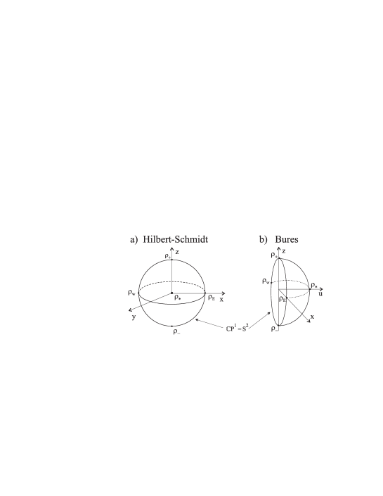
Figure 1: Geometry of the set of the mixed states for $N=2$: a) – the $3$-ball embedded in ${\mathbb{R}}^{3}$ induced by the Hilbert-Schmidt distance, b) – hemisphere of ${\bf S}^{3}$ embedded in ${\mathbb{R}}^{4}$, (shown as a cross-section of $R^{4}$ taken at $y=0$), induced by the Bures distance. The maximally mixed state $\rho_{*}$ is located at the center of the ball (a), and at the hyper-pole of ${\bf S}^{3}$ (b). The set of pure states is represented by the Bloch sphere ${\bf S}^{2}$ (a) and by the Uhlmann equator ${\bf S}^{2}\in{\bf S}^{3}$ (b). The cross-section of ${\cal M}_{2}$ with the plane $z=0$ produces a full circle in the equatorial plane (a), or a half of a hyper-meridian joining the states $\rho_{W}$ and $\rho_{E}$ (b).

Working in a Cartesian coordinate system we may rewrite (11) as

$${\rho}=\frac{1}{2}\left(\begin{array}[]{cc}1+z&x-iy\\ x+iy&1-z\end{array}\right)\ ,\hskip 28.45274ptx^{2}+y^{2}+z^{2}\leq 1\$$ (12)

Setting ${\rho}_{A}=\rho$, $\rho_{B}=\rho+{\rm d}\rho$ in the expression for the Bures distance (6) and expanding to second order we obtain one–fourth times the round metric on the 3-sphere,

$${\rm d}s^{2}_{B}=\frac{1}{4}\left(dx^{2}+dy^{2}+dz^{2}+\frac{(xdx+ydy+zdz)^{2}}{1-x^{2}-y^{2}-z^{2}}\right)\ .$$ (13)

Uhlmann noticed this fact in Uh92 and suggested embedding of the three dimensional space of the $N=2$ mixed states in ${\mathbb{R}}^{4}$. The transformation

$$\rho(x,y,z)\to{\frac{1}{2}}\Bigl{(}x,y,z,u:=\sqrt{1-x^{2}-y^{2}-z^{2}}\Bigr{)}$$ (14)

blows up the $3$-ball into the Uhlmann hyper-hemisphere of ${\bf S}^{3}$ of radius $R_{2}=1/2$. The maximally mixed state $\rho_{*}$, mapped into a hyper-pole, is equally distant from all pure states located at the hyper-equator - see Fig. 1. The hyper-equator is equivalent to an ordinary two dimensional sphere and hence isometric to ${\mathbb{C}}P^{1}$. The comparison between both metrics is very transparent for real density matrices: the space of all rebits, which in the HS-metric has the structure of the $2$-ball, in the Bures metric has the from of a hemisphere of ${\bf S}^{2}$.

Since the radius $R_{B}$ of the Uhlmann hemisphere is equal to $1/2$ we obtain immediately the Bures volume $V$ and the Bures area $S$ for $N=2$

$$V_{2}^{(2)}={\mbox{vol}_{B}}\bigl{(}{\cal M}_{2}\bigr{)}=\frac{1}{2}S_{3}R_{B}^{3}=\frac{\pi^{2}}{8}\ ,\quad\quad S_{2}^{(2)}={\mbox{vol}_{B}}\bigl{(}\partial{\cal M}_{2}\bigr{)}=S_{2}R_{B}^{2}=\pi,$$ (15)

where $S_{k}$ denotes the volume of the unit sphere ${\bf S}^{k}$. This result was obtained by Caves Ca02 , who also expressed the Bures volume of the set of mixed states in form of an integral. In the further sections of our work we are going to compute such integrals to derive an explicit result for the Bures volume for an arbitrary matrix size $N$.

The last property of the Bures metric, we are going to review, concerns monotonicity. In the classical case of commuting diagonal density matrices, one studies the space of probability vectors ${\vec{a}}=\{a_{1},...a_{N}\}$, where $a_{i}\geq 0$ and $\sum_{i=1}^{N}a_{i}=1$. This space is isomorphic with an $N-1$ dimensional simplex $\Delta_{N-1}$. A discrete dynamics in this space, ${\vec{a}}^{\prime}=T{\vec{a}}$, is given by an arbitrary stochastic matrix $T$ of size $N$. This matrix contains non–negative entries, $T_{ij}\geq 0$, and the stochasticity condition, $\sum_{j=1}^{N}T_{ji}=1$ for $i=1,...,N$ assures that the output vector ${\vec{a}}^{\prime}$ is normalized. A distance in the space $\Delta_{N-1}$ of $N$–dimensional probability vectors is called monotone, if it does not increase under the action of any stochastic matrix $T$,

$$D_{\rm mon}\bigr{(}{\vec{a}},{\vec{b}}\bigl{)}\ \geq\ D_{\rm mon}\bigr{(}T{\vec{a}},T{\vec{b}}\bigl{)}.$$ (16)

If a geodesic distance in the probability simplex is monotone, the corresponding Riemannian metric is called monotone. Chentsov showed Ce82 that every monotone Riemannian distance in this space is a function of the Fisher statistical distance Fi25 , or the Bhattacharyya coefficient $B$ defined in (7).

The quantum case is more complicated. Any discrete dynamics may be described by a quantum operation, $\Phi:{\cal M}_{N}\to{\cal M}_{N}$, which is trace preserving, Tr$\Phi(\rho)={\rm Tr}\rho=1$, and completely positive. Positivity means that $\Phi(\rho)\geq 0$, i.e. $\Phi$ sends positive operators into positive operators. From a physical point of view it is necessary to assure that an operation is well defined on the system coupled to an ancilla - an auxiliary system which describes the environment. Hence one requires that $\Phi$ is completely positive, which means that any extension of the map by an identity operator, $\Phi\otimes{\mathbb{I}}$, is positive OP93 . Completely positive trace preserving maps play the role of stochastic matrices $T$ in the quantum case, and are thus called stochastic maps. In full analogy to (16) any distance $D$ in the space of mixed quantum states ${\cal M}^{(N)}$ is called monotone if it does not grow under the action of a stochastic map,

$$D_{\rm mon}\bigr{(}\rho,\sigma\bigl{)}\geq D_{\rm mon}\bigr{(}\Phi(\rho),\Phi(\sigma)\bigl{)}\ .$$ (17)

If a monotone distance is geodesic the corresponding metric on ${\cal M}_{N}$ is called monotone.

Figure 2: Morozova–Chentsov functions $f(t)$: minimal function for maximal metric (dotted line), Kubo–Mori metric (dashed line), and maximal function for the minimal, Bures metric (upper line). These metrics are Fisher–adjusted, $f(1)=1$, while Bures metric is also Fubini–Study adjusted, $f(0)=1/2$.

In contrast to the classical case, there exist infinitely many monotone Riemannian metrics on the space of mixed quantum states. However, as shown by Morozova and Chentsov MC90 and Petz and Sudár PS96 , they may be characterized by a symmetric function $c(x,y)$. In general, the length of a vector (matrix) $B_{ij}$ may be position dependent; at a diagonal point $A={\rm diag}(a_{1},a_{2},...,a_{N})$ the squared length of $B$ is given by PS96

$$||B||^{2}_{A}=\sum_{j=1}^{N}\frac{B_{jj}}{a_{j}}+2\sum_{j<k=1}^{N}c(a_{j},a_{k})|B_{jk}|^{2}\ .$$ (18)

For a diagonal matrix $B$ the second term vanishes and the first term gives back the unique statistical metric on the simplex. The off–diagonal elements, which enter the second term in (18), allow for more freedom in the choice of a monotone Riemannian metric. The Morozova-Chentsov function satisfies $c(sx,sy)=s^{-1}c(x,y)$. The symmetry of this two–argument function $c$ enables to express it by a function of a single parameter, $c(x,y)=f(x/y)/y$, such that $f(1/t)=f(t)/t$.

A function $f$ is called operator monotone, if for any matrices $G$, $H$ the relation $0\leq G\leq H$ implies $0\leq f(G)\leq f(H)$. Here $G\leq H$ denotes that their difference is semi positive, $H-G\geq 0$. Taking for $G$ and $H$ real numbers we see that operator monotonicity implies that $f$ maps ${\mathbb{R}}_{+}\to{\mathbb{R}}_{+}$ and is concave. The result of Morozova and Chentsov MC90 , completed and extended by Petz and Sudár Pe96 ; PS96 , states that every monotone metric may be written in the form (18) up a proportionality constant. Conversely, this equation determines a monotone Riemannian metric, if the function $f(t)=1/c(t,1)$ is: a) operator monotone, and b) self–transposed, $f(1/t)=f(t)/t$. Such functions $f$ are called Morozova–Chentsov functions. Comparison of different metrics is meaningful under a certain normalization. Usually one requires: c) $f(1)=1$, since for diagonal matrices such a metric agrees with the statistical (Fisher) metric, and is called Fisher–adjusted. There exists infinitely many functions $f$ satisfying all three conditions a)–c), and leading to Fisher–adjusted metrics PS96 . Let us mention three examples here:

$$f_{\rm min}(t)=\frac{2t}{t+1},{\quad\quad}f_{\rm KM}(t)=\frac{t-1}{\ln t},{\quad\quad}f_{\rm max}(t)=\frac{1+t}{2}$$ (19)

containing both extremal cases and the intermediate Kubo-Mori (Bogolioubov) metric used in quantum statistical mechanics BAR86 and distinguished by the fact that both affine connections with respect to this metric are mutually dual GS01 . These functions, plotted in Fig. 2, correspond to

$$c_{\rm min}(x,y)=\frac{x+y}{2xy},{\quad\quad}c_{\rm KM}(x,y)=\frac{\ln x-\ln y}{x-y},{\quad\quad}c_{\rm max}(x,y)=\frac{2}{x+y},$$ (20)

so the inverse, $1/c$, is equal to the harmonic, logarithmic and arithmetic mean, respectively. It is known that among all normalised, self-transposed, operator monotone functions $f$ there is a minimal and a maximal one KA80 . They are distinguished above by the appropriate labels. The maximal concave function $f_{\rm max}(t)$, the straight line $t/2+1/2$, induces the Bures metric and the Bures distance PS96 ; LR99 .

If $f(0)=1/2$ the metric induces the natural Riemannian metric on the subspace ${\mathbb{C}}P^{N-1}$ of pure states and is called Fubini-Study adjusted Uh95 ; PS96 . The Bures metric is the only monotone metric which is simultaneously Fisher–adjusted and Fubini–Study–adjusted. This property, valid for any matrix size $N$, is easiest to discuss for $N=2$. All metrics defined by (18) are rotationally invariant, i.e. the uniform angular distribution (of eigenvectors of the density matrix) is independent of the radial distribution (of its eigenvalues). In the one–qubit case the metric depends only on the radius $r=\sqrt{x^{2}+y^{2}+z^{2}}$ in the unit Bloch ball, and may be divided into the radial and the normal (tangential) components Pe96 ,

$${\rm d}s^{2}=\frac{1}{1-r^{2}}{\rm d}r^{2}+\frac{1}{1+r}g\Bigl{(}\frac{1-r}{1+r}\Bigr{)}{\rm d}n^{2}\quad{\rm with\quad}g(t)=\frac{1}{f(t)}$$ (21)

The radial component is independent of the function $f$. It is easy to see that the value of $f(t)$ at $t=0$ determines the metric at the subspace of pure states, $r=1$. If $f(0)=0$, then the metric diverges at the manifold of pure states, which is the case for $f_{\rm KM}$ and $f_{\rm min}$.

The relation between the Morozova-Chentsov function and the metric $g=1/f$ shows that the larger the (normalized) function $f$, the smaller the metric and the corresponding distance. The Bures metric given by the maximal function $f_{\rm max}(t)$, is therefore the minimal Fisher–adjusted, monotone Riemannian metric. These properties single out the Bures metric and provide an additional motivation to study the geometry it induces in the set of mixed quantum states.

III Bures measure

III.1 Infinitesimal distance

We are going to compute the Bures distance (6) between two infinitesimally close density matrices of size $N$. Let us set $\rho_{A}=\rho,\ \rho_{B}=\rho+\delta\rho$:

$$\sqrt{\rho_{A}^{1/2}\rho_{B}\ \rho_{A}^{1/2}}=\rho+X+Y$$ (22)

where the matrix $X$ is of order $1$ in $\delta\rho$, while $Y$ is of order $2$. Squaring this equation we obtain to first and second order

$$\rho^{1/2}\delta\rho\ \rho^{1/2}=X\rho+\rho X\ ,\ \ \ \ \ \ -X^{2}=Y\rho+\rho Y$$ (23)

or in the basis in which $\rho$ is diagonal with eigenvalues $\rho_{\nu}>0$

$$X_{\nu\mu}=\delta\rho_{\nu\mu}\ \frac{\rho_{\nu}^{1/2}\rho_{\mu}^{1/2}}{\rho_{\nu}+\rho_{\mu}}\ ,\quad\quad Y_{\nu\mu}=-(X^{2})_{\nu\mu}\frac{1}{\rho_{\nu}+\rho_{\mu}}\ .$$ (24)

Since ${\rm Tr}\rho=1$, hence ${\rm Tr}\delta\rho=0$ and ${\rm Tr}X={\rm Tr}\ \delta\rho/2=0$, while

$${\rm Tr}Y=-\sum_{\nu\mu}{1\over 2\rho_{\nu}}|X_{\nu\mu}|^{2}=-\sum_{\nu\mu}{1\over 4}{|\delta\rho_{\nu\mu}|^{2}\over{\rho_{\nu}+\rho_{\mu}}}\ .$$ (25)

Thus we arrive at the result of Hübner Hu92 for the Bures metric

$$({\rm d}s)_{B}^{2}=(D(\rho,\rho+\delta\rho))^{2}={1\over 2}\sum_{\nu\mu}{|\delta\rho_{\nu\mu}|^{2}\over{\rho_{\nu}+\rho_{\mu}}}\ .$$ (26)

Note, that if $\rho_{\nu}=0$ and $\rho_{\mu}=0$, $\delta\rho_{\nu\mu}$ does not appear and therefore terms where the denominator vanishes have to be excluded.

III.2 The volume

Let us rewrite the metric (26) distinguishing the diagonal elements

$$({\rm d}s)_{B}^{2}=\sum_{\nu=1}^{N}{|\delta\rho_{\nu\nu}|^{2}\over{4\rho_{\nu}}}+\sum_{\nu<\mu}{|\delta\rho_{\nu\mu}|^{2}\over{\rho_{\nu}+\rho_{\mu}}}\ .$$ (27)

For diagonal matrices the second term vanishes and the above expression reduces to (10). Since ${\rm Tr}\rho=1$ so $\sum_{\nu=1}^{N}{\delta\rho_{\nu\nu}}=0$ and not all $\delta\rho_{\nu\nu}$ are independent. Eliminating $\delta\rho_{NN}$ we obtain

$$\sum_{\nu=1}^{N}{(\delta\rho_{\nu\nu})^{2}\over{\rho_{\nu}}}=\sum_{\nu=1}^{N-1}{{(\delta\rho_{\nu\nu})}^{2}\over{\rho_{\nu}}}+(\sum_{\nu=1}^{N-1}{\delta\rho_{\nu\nu}})^{2}{1\over\rho_{N}}\ .$$ (28)

The metric (28) in the $(N-1)$–dimensional subspace is of the form $g_{ik}=(\delta_{ik}/\rho_{i}+1/\rho_{N})$ with determinant $\det g=(\rho_{1}+\rho_{2}+...+\rho_{N})/(\rho_{1}\rho_{2}...\rho_{N})=1/\det\rho$ using ${\rm Tr}\rho=1$. Thus the volume element gains a factor $\sqrt{{\rm det}g}=(\det\rho)^{-1/2}$:

$${\rm d}V_{B}={1\over 2^{{N^{2}}-1}}(\det\rho)^{-1/2}\prod_{\nu=1}^{N-1}{\rm d}\rho_{\nu\nu}\ \prod_{\nu<\mu}{2\over\rho_{\nu}+\rho_{\mu}}\ \prod_{\nu<\mu}\bigl{(}\sqrt{2}\ {\rm d}{\rm Re}(\rho_{\nu\mu})\sqrt{2}\ {\rm d}{\rm Im}(\rho_{\nu\mu})\bigr{)}\ .$$ (29)

The total volume of the set ${\cal M}_{N}$ is given by:

$$V_{B}={2^{1-{N^{2}}}}\int D\rho\ {\delta({\rm Tr}\rho-1)\over{\det\rho^{1/2}}}\theta(\rho)\prod_{\nu<\mu}{2\over{\rho_{\nu}+\rho_{\mu}}}\$$ (30)

with $\theta(\rho)=\theta(\rho_{1})...\theta(\rho_{N})$ a step function that restricts integration to nonnegative $\rho$. We introduced the volume element

$$D\rho=\prod_{\nu=1}^{N}{\rm d}\rho_{\nu\nu}\prod_{\nu<\mu}\bigl{(}\sqrt{2}\ {\rm dRe}(\rho_{\nu\mu})\sqrt{2}\ {\rm dIm}(\rho_{\nu\mu})\bigr{)}\ .$$ (31)

which differs from the usual definition by a factor $2^{N(N-1)/2}$. It follows from the metric for unrestricted Hermitian matrices:

$$({\rm d}s)^{2}=\sum_{\nu=1}^{N}{(\delta\rho_{\nu\nu})^{2}}+2\sum_{\nu<\mu}{|\delta\rho_{\nu\mu}|^{2}}\ .$$ (32)

Above we considered the case of Hermitian density matrices ($\beta=2$). In the case of real density matrices ($\beta=1$) there are no imaginary parts ${\rm Im}\rho_{\nu\mu}$.

III.3 Radial coordinates

Let us diagonalize the matrices $\rho$

$$\rho=U\Lambda U^{-1}\quad{\rm or}\quad\rho=O\Lambda O^{-1}\ \$$ (33)

with $U$ unitary for $\beta=2$, $O$ orthogonal for $\beta=1$, $\Lambda={\rm diag}(\rho_{1},\rho_{2},...,\rho_{N})$. Then we have

$${\rm d}\rho=U[{\rm d}\Lambda+U^{-1}{\rm d}U\Lambda-\Lambda U^{-1}{\rm d}U]U^{-1}\ {\rm or}\ {\rm d}\rho=O[{\rm d}\Lambda+O^{-1}{\rm d}O\Lambda-\Lambda O^{-1}{\rm d}O]O^{-1}\ \ .$$ (34)

Let us first rewrite the Bures metric in a basis independent way,

$$({\rm d}s)_{B}^{2}={1\over 2}\int_{0}^{\infty}{\rm d}t\ {\rm Tr}({\rm d}\rho{\rm e}^{-\rho t}{\rm d}\rho{\rm e}^{-\rho t})\ .$$ (35)

This means it contains left and right multiplications with $\rho$. Inserting now the expressions for d$\rho$ we see that again we can go to the representation where $\rho$ is diagonal and obtain metrics in the cases of complex density matrices,

$$({\rm d}s)^{2}=\sum_{\nu=1}^{N}\frac{({\rm d}\rho_{\nu})^{2}}{4\rho_{\nu}}+\sum_{\nu<\mu}{(\rho_{\nu}-\rho_{\mu})^{2}\over{\rho_{\nu}+\rho_{\mu}}}|(U^{-1}{\rm d}U)_{\nu\mu}|^{2}\ ,$$ (36)

and real density matrices

$$({\rm d}s)^{2}=\sum_{\nu=1}^{N}\frac{({\rm d}\rho_{\nu})^{2}}{4\rho_{\nu}}+\sum_{\nu<\mu}{(\rho_{\nu}-\rho_{\mu})^{2}\over{\rho_{\nu}+\rho_{\mu}}}|(O^{-1}{\rm d}O)_{\nu\mu}|^{2}\ .$$ (37)

In both cases the Bures measure has the following product form

$${\rm d}V_{B}^{(\beta)}={\rm d}\mu^{(\beta)}(\rho_{1},\rho_{2},...,\rho_{N})\times{\rm d}\nu_{\beta}.$$ (38)

The first factor depends only on the eigenvalues $\rho_{i}$, while the latter, determining the distribution of the eigenvectors of the density matrix, is the unique, unitarily invariant, Haar measure on $U(N)$ for $\beta=2$ or on $O(N)$ for $\beta=1$. In the general case of complex density matrices, ($\beta=2)$, the Bures measure in the simplex of eigenvalues reads

$$P_{B}(\Lambda)=P_{B}(\rho_{1},\rho_{2},...,\rho_{N})=C_{N}\frac{\delta\bigl{(}\rho_{1}+\rho_{2}+...+\rho_{N}-1)}{\sqrt{\rho_{1}\rho_{2}\cdots\rho_{N}}}\prod_{\nu<\mu}\frac{(\rho_{\nu}-\rho_{\mu})^{2}}{\rho_{\nu}+\rho_{\mu}},$$ (39)

where the normalization constant $C_{N}$ assures that the integral of $P$ over all eigenvalues equals to unity. The measure was derived by Hall Ha98 , and was later analyzed in BS01 ; ZS01 . To compute the area of the surface of the set of complex density matrices, and to find the volume of the set of real density matrices we will need a family of generalized constants $C_{N}(\alpha,\beta)$ defined by

$${1\over C_{N}(\alpha,\beta)}=\int_{0}^{\infty}\prod_{\nu=1}^{N}{{\rm d}\rho_{\nu}\over\rho_{\nu}^{1/2}}\ {\delta(\rho_{1}+...+\rho_{N}-1)}\left[\prod_{\nu<\mu}^{1...N}{(\rho_{\nu}-\rho_{\mu})^{2}\over\rho_{\nu}+\rho_{\mu}}\right]^{\beta/2}\prod_{\kappa={1}}^{N}\rho_{\kappa}^{\alpha-1}\ .$$ (40)

The standard Hall constants entering (39) become a special case of this definition, $C_{N}=C_{N}(1,2)$. They will be needed to compute the Bures volume of ${\cal M}_{N}$.

Integrating the Bures measure over the eigenvectors distributed according to the Haar measure on $U(N)$ or $O(N)$ we obtain

$$dV_{B}^{(\beta)}=2^{1-N[1+(N-1)\beta/2]}\det\rho^{-1/2}\prod_{\nu=1}^{N-1}{\rm d}\rho_{\nu}\ \prod_{\nu<\mu}\left[{2(\rho_{\nu}-\rho_{\mu})^{2}\over\rho_{\nu}+\rho_{\mu}}\right]^{\beta/2}\ V_{\rm Flag}^{(\beta)}(N)\ .$$ (41)

where $V_{\rm Flag}^{(\beta)}(N)$ denotes the volume of the flag manifold, $Fl_{N}^{\mathbb{C}}=U(N)/U(1)^{N}$ or $Fl_{N}^{\mathbb{R}}=O(N)/O(1)^{N}$ for $\beta=2,1$. Although these volumes

$$V_{\rm Flag}^{(2)}(N)={\rm Vol}\bigl{(}Fl_{N}^{\mathbb{C}}\bigr{)}={(2\pi)^{N(N-1)/2}\over\Gamma(1)\Gamma(2)...\Gamma(N)}\quad{\rm and}\quad V_{\rm Flag}^{(1)}(N)={\rm Vol}\bigl{(}Fl_{N}^{\mathbb{R}}\bigr{)}={(2\pi)^{N(N-1)/4}\pi^{N/2}\over\Gamma(1/2)\Gamma(2/2)...\Gamma(N/2)}\$$ (42)

were computed by Hua several years ago Hu63 , we provide their short derivation in ZS03 and show that various results for the volumes of the unitary groups and flag manifolds present in the literature Fu01 ; BST02 ; TS02 ; Ca02 are due to different choice of normalization. Formally we may write the volumes in the form:

$$V_{\rm Flag}^{(\beta)}(N)=\prod_{j=1}^{N}(2\pi)^{(j-1)\beta/2}\frac{\Gamma(\beta/2)}{\Gamma(j\beta/2)}\ ,$$ (43)

which shows that it is the product of the volumes of projective spaces with increasing dimension $j-1$, real for $\beta=1$, complex for $\beta=2$, and the radius rescaled by a factor $\sqrt{2}$ coming from the factor $2^{\beta N(N-1)/4}$ – see appendix of ZS03 .

Since the unitary or orthogonal rotations produce all permutations, in (41) we have to restrict to a certain order of eigenvalues, $\rho_{1}<\rho_{2}<...<\rho_{N}$. In order to lift this condition we need to divide the result by the number of permutations, equal to $N!$,

$$V_{B}^{(\beta)}=2^{1-N[1+(N-1)\beta/2]}\int_{0}^{\infty}{{\rm d}\rho_{1}...{\rm d}\rho_{N}\over\det\rho^{1/2}}\delta({\rm Tr}\rho-1)\ \prod_{\nu<\mu}\left[{2(\rho_{\nu}-\rho_{\mu})^{2}\over\rho_{\nu}+\rho_{\mu}}\right]^{\beta/2}\ {V_{\rm Flag}^{(\beta)}(N)\over N!}\ .$$ (44)

III.4 The surface

The surface consists of the N pieces with one eigenvalue $=0$. To calculate the metric on the surface (with $\rho_{1}=0$) we put first ${\rm d}\rho_{1}=0$ and then $\rho_{1}=0$ (remember that terms with vanishing denominator have to be excluded):

$$({\rm d}s)^{2}=\sum_{\nu=2}^{N}{({\rm d}\rho_{\nu})^{2}\over{4\rho_{\nu}}}+\sum_{\nu<\mu}^{2...N}{(\rho_{\nu}-\rho_{\mu})^{2}\over{\rho_{\nu}+\rho_{\mu}}}|(U^{-1}{\rm d}U)_{\nu\mu}|^{2}+\sum_{\mu=2}^{N}\rho_{\mu}|(U^{-1}{\rm d}U)_{1\mu}|^{2}\ .$$ (45)

Then with the same reasoning as above the surface element is given by

$${\rm d}S=2^{1-(N-1)(1+N\beta/2)}\prod_{\nu=2}^{N-1}{{\rm d}\rho_{\nu}\over\rho_{\nu}^{1/2}}\ \left[\prod_{\nu<\mu}^{2...N}{2(\rho_{\nu}-\rho_{\mu})^{2}\over\rho_{\nu}+\rho_{\mu}}\prod_{\kappa=2}^{N}2\rho_{\kappa}\right]^{\beta/2}\ V_{\rm Flag}^{(\beta)}(N)\$$ (46)

and the total surface:

$$S_{N}^{(\beta)}=S_{N,1}^{(\beta)}=2^{1-(N-1)(1+N\beta/2)}\int\prod_{\nu=2}^{N}{{\rm d}\rho_{\nu}\over\rho_{\nu}^{1/2}}\ {\delta(\rho_{2}+...+\rho_{N}-1)\over(N-1)!}\left[\prod_{\nu<\mu}^{2...N}{2(\rho_{\nu}-\rho_{\mu})^{2}\over\rho_{\nu}+\rho_{\mu}}\prod_{\kappa=2}^{N}2\rho_{\kappa}\right]^{\beta/2}\ V_{\rm Flag}^{(\beta)}(N)\ ,$$ (47)

where we have taken into account all permutations of the $N-1$ non–zero eigenvalues.

III.5 The edges and hyperedges

There are $N(N-1)/2$ edges which correspond to two vanishing eigenvalues. Hence there are $(N-2)!$ different permutations of positive, generically different eigenvalues which form the edges. To calculate the metric on the edges we put first ${\rm d}\rho_{1}={\rm d}\rho_{2}=0$ and then $\rho_{1}=\rho_{2}=0$:

$$({\rm d}s)^{2}=\sum_{\nu=3}^{N}{({\rm d}\rho_{\nu})^{2}\over{4\rho_{\nu}}}+\sum_{\nu<\mu}^{3...N}{(\rho_{\nu}-\rho_{\mu})^{2}\over{\rho_{\nu}+\rho_{\mu}}}|(U^{-1}{\rm d}U)_{\nu\mu}|^{2}+\sum_{\mu=3}^{N}\rho_{\mu}(|(U^{-1}{\rm d}U)_{1\mu}|^{2}+|(U^{-1}{\rm d}U)_{2\mu}|^{2})\ .$$ (48)

We see that there do not appear terms $(U^{-1}{\rm d}U)_{\nu\mu}$ with $\nu,\mu=1,2$. Thus the corresponding coset space which has to be integrated over is the flag manifold $U(N)/[U(2)\times U(1)^{N-2}]$ for $\beta=2$ or $O(N)/[O(2)\times O(1)^{N-2}]$ for $\beta=1$. Since their volume is equal to the ratio Vol$(Fl_{N})/{\rm Vol}(Fl_{2})$, the edge element is then given by

$${\rm d}S_{N,2}^{(\beta)}={2^{-d_{2}}}\prod_{\nu=3}^{N-1}{{\rm d}\rho_{\nu}\over\rho_{\nu}^{1/2}}\ \left[\prod_{\nu<\mu}^{3...N}{2(\rho_{\nu}-\rho_{\mu})^{2}\over\rho_{\nu}+\rho_{\mu}}\prod_{\kappa=3}^{N}(2\rho_{\kappa})^{2}\right]^{\beta/2}\ {V_{\rm Flag}^{(\beta)}(N)\over V_{\rm Flag}^{(\beta)}(2)}\$$ (49)

with the dimension $d_{n}$

$$d_{n}=(N-n)(1+(N+n-1)\beta/2)-1\ .$$ (50)

The total area of the edges is

$$S_{N,2}^{(\beta)}={2^{-d_{2}}}\int_{0}^{\infty}\prod_{\nu=3}^{N}{{\rm d}\rho_{\nu}\over\rho_{\nu}^{1/2}}\ {\delta(\rho_{3}+...+\rho_{N}-1)\over(N-2)!}\left[\prod_{\nu<\mu}^{3...N}{2(\rho_{\nu}-\rho_{\mu})^{2}\over\rho_{\nu}+\rho_{\mu}}\prod_{\kappa=3}^{N}(2\rho_{\kappa})^{2}\right]^{\beta/2}\ {V_{\rm Flag}^{(\beta)}(N)\over V_{\rm Flag}^{(\beta)}(2)}\ .$$ (51)

It is straightforward to generalize this to hyperedges: the manifold of states of rank $N-n$ with $n=0,1,...N-1$ has the volume

$$S^{(\beta)}_{N,n}={2^{-d_{n}}}\int_{0}^{\infty}\prod_{\nu=n+1}^{N}{{\rm d}\rho_{\nu}\over\rho_{\nu}^{1/2}}\ {\delta(\rho_{n+1}+...+\rho_{N}-1)\over(N-n)!}\left[\prod_{\nu<\mu}^{n+1...N}{2(\rho_{\nu}-\rho_{\mu})^{2}\over\rho_{\nu}+\rho_{\mu}}\prod_{\kappa={n+1}}^{N}(2\rho_{\kappa})^{n}\right]^{\beta/2}\ {V_{\rm Flag}^{(\beta)}(N)\over V_{\rm Flag}^{(\beta)}(n)}\ .$$ (52)

IV Bures volume

IV.1 Normalization constants

The above formulae for the volumes of manifolds of states of rank $N-n$ may be expressed in a compact way with use of the generalized Hall constants (40)

$$S^{(\beta)}_{N,n}={2^{-d_{n}+(N-n)(N+n-1)\beta/4}\over(N-n)!C_{N-n}(1+n\beta/2,\ \beta)}\ {V_{\rm Flag}^{(\beta)}(N)\over V_{\rm Flag}^{(\beta)}(n)}\ .$$ (53)

We are going to compute the constants $C_{N}(\alpha,\beta)$ for integer $\alpha,\beta$ and then continue analytically to general positive $\alpha$ and $\beta$. Let us go to variables $\rho_{i}=t_{i}^{2}$. Then the integral (40) is an integral over the full sphere $R^{2}=t_{1}^{2}+t_{2}^{2}+...+t_{N}^{2}=1$ with an homogeneous function in R of order $\beta N(N-1)/2+2N(\alpha-1)$ as integrand. The radial integral may be replaced by a $\Gamma$ function, which amounts to replacing $\delta(R^{2}-1)$ by ${\rm e}^{-R^{2}}$. The result is the same up to a factor. Afterwards we may go back to the variables $\rho_{i}$ and obtain

$${\Gamma[N(2\alpha+(N-1)\beta/2-1)/2]\over C_{N}(\alpha,\beta)}=\int_{0}^{\infty}\prod_{\nu=1}^{N}{{\rm d}\rho_{\nu}\over\rho_{\nu}^{1/2}}\ {\rm e}^{-(\rho_{1}+...+\rho_{N})}\left[\prod_{\nu<\mu}^{1...N}{(\rho_{\nu}-\rho_{\mu})^{2}\over\rho_{\nu}+\rho_{\mu}}\right]^{\beta/2}\prod_{\kappa={1}}^{N}\rho_{\kappa}^{\alpha-1}\ .$$ (54)

In the next step we want to eliminate the denominators in (54). In this section we discuss the case $\beta=2$ of complex density matrices,

$${1\over(\rho_{1}...\rho_{N})^{1/2}}\prod_{\nu<\mu}{1\over\rho_{\nu}+\rho_{\mu}}=\int{\rm e}^{-\sum\rho_{i}X_{ii}^{2}-\sum_{i<j}|X_{ij}|^{2}(\rho_{i}+\rho_{j})}\prod_{i=1}^{N}{{\rm d}X_{ii}\over\sqrt{\pi}}\prod_{i<j}{{\rm d\ Re}X_{ij}~{}{\rm d\ Im}X_{ij}\over\pi}$$ (55)

Using the volume element $DX$ of a Hermitian Matrix X (31) we may rewrite this as

$${1\over(\rho_{1}...\rho_{N})^{1/2}}\prod_{\nu<\mu}{1\over\rho_{\nu}+\rho_{\mu}}=\pi^{-N^{2}/2}\ 2^{-N(N-1)/2}\ \int DX\ {\rm e}^{-{\rm Tr}\ \rho X^{2}}\ .$$ (56)

This expression is basis independent and provides a way to describe the Bures probability distribution in a random matrix description. With this we may write for $\beta=2$

$${\Gamma(N^{2}/2+N(\alpha-1))\over C_{N}(\alpha,2)}=\pi^{-N^{2}/2}\ 2^{-N(N-1)/2}{N!\over V_{\rm Flag}^{(2)}(N)}\ \int D\rho\ \theta(\rho)\det\rho^{\alpha-1}\ \int DX\ {\rm e}^{-{\rm Tr}\ \rho(1+X^{2})}\ .$$ (57)

Now we use a formula which is an extension of the Ingham-Siegel integral Fy02

$$\left[\det\left({\delta\over\delta\rho}\ +\epsilon\right)\right]^{-N}\ \delta(\rho)=A_{N}\theta(\rho)\ {\rm e}^{-{\rm Tr}\ \epsilon\rho}\$$ (58)

valid for a positive Hermitian matrix $\epsilon$ and with a constant $A_{N}$. Let us derive this formula:

$$\left[\det\left({\delta\over\delta\rho}\ +\epsilon\right)\right]^{-N}\ \delta(\rho)=\pi^{-N^{2}}\int{\rm d}\psi_{1}...{\rm d}\psi_{N}\ {\rm e}^{-[\psi_{1}^{\dagger}(\delta/\delta\rho+\epsilon)\psi_{1}+...+\psi_{N}^{\dagger}(\delta/\delta\rho+\epsilon)\psi_{N}]}\ \delta(\rho)\$$ (59)

with $N$-dimensional complex vectors $\psi_{1},...,\psi_{N}$. The translation operator shifts the argument $\rho$ of the $\delta$–function by the matrix $\psi_{1}\otimes\psi_{1}^{\dagger}+...+\psi_{N}\otimes\psi_{N}^{\dagger}$. Then the integration can be done and yields

$$\left[\det\left({\delta\over\delta\rho}\ +\epsilon\right)\right]^{-N}\ \delta(\rho)={\rm e}^{-{\rm Tr}\ \epsilon\rho}\ \pi^{-N^{2}}\ \int{\rm d}\psi_{1}...{\rm d}\psi_{N}\ \delta(\rho-(\psi_{1}\otimes\psi_{1}^{\dagger}+...+\psi_{N}\otimes\psi_{N}^{\dagger}))\ .$$

For $\rho>0$ we may rescale $\psi\to\sqrt{\rho}\psi$. The Jacobian cancels out and the result is equation (58). The constant $A_{N}$ can be calculated from integrating this equation (58) over $\rho$. With partial integration we find

$${2^{N(N-1)/2}\over\det\epsilon^{N}}=A_{N}\ \int D\rho\ \theta(\rho)\ {\rm e}^{-{\rm Tr}\ \epsilon\rho}\ .$$

This is valid for any Hermitian matrix $\epsilon>0$. The coefficient $A_{N}$ is independent of the matrix $\epsilon$. To calculate $A_{N}$ we put $\epsilon={\mathbb{I}}$. The integral can again be done using the Laguerre ensemble:

$${1\over A_{N}}={V_{\rm Flag}^{(2)}(N)\over 2^{N(N-1)/2}N!}\ \prod_{j=1}^{N}\ \Gamma(1+j)\Gamma(j)=\pi^{N(N-1)/2}\ \Gamma(1)...\Gamma(N)\ .$$ (60)

IV.2 Main results

Using equations (57, 58, 60) we may write

$${\Gamma(N^{2}/2+N(\alpha-1))\over C_{N}(\alpha,2)}={\pi^{-N^{2}/2}\ 2^{-N(N-1)/2}\over A_{N}}{N!\over V_{\rm Flag}^{(2)}(N)}\ \int D\rho\int DA\ \det\rho^{\alpha-1}\ \left[\det\left({\delta\over\delta\rho}+1+A^{2}\right)\right]^{-N}\ \delta(\rho)\ .$$ (61)

For $\alpha=1$ we obtain immediately by partial integration:

$${\Gamma(N^{2}/2)\over C_{N}(1,2)}={\pi^{-N^{2}/2}N!\over A_{N}V_{\rm Flag}^{(2)}(N)}\ \int{DA\over\det(1+A^{2})^{N}}\ ={\pi^{-N^{2}/2}\over A_{N}}\int\prod_{i=1}^{N}{{\rm d}a_{i}\over(1+a_{i}^{2})^{N}}\ \prod_{i<j}(a_{i}-a_{j})^{2}\ .$$ (62)

The last integral may be calculated in the complex plane and yields: $(2\pi)^{N}N!2^{-N^{2}}$, such that the Bures–Hall constants are given by

$$C_{N}=C_{N}(1,2)={2^{N^{2}-N}\ \Gamma(N^{2}/2)\over\pi^{N/2}\ \Gamma(1)...\Gamma(N+1)}\ .$$ (63)

This coincides with the known values for the Bures–Hall constants, $C_{2}=2/\pi$, $C_{3}=35/\pi$ and $C_{4}=2^{11}35/\pi^{2}$ and confirms some conjectures of Slater concerning $C_{5}$ and $C_{6}$ Sl99b . The Bures volume of the set of complex density matrices of size $N$ is now given by

$$V_{N}^{(2)}={2^{1-N(N+1)/2}\over C_{N}(1,2)}\ {V_{\rm Flag}^{(2)}(N)\over N!}=2^{1-N^{2}}{\pi^{N^{2}/2}\over\Gamma(N^{2}/2)}$$ (64)

and for $N=2$ reduces to (15). Note that the factor $2^{1-N^{2}}$ enters from the beginning in the definition. It disappears, if we increase d$s$ (27) by a factor of $2$. The Bures volume is exactly equal to the $(N^{2}-1)$-dimensional volume of an $(N^{2}-1)$ dimensional hemisphere with radius $1/2$. Equations (63) and (64) constitute the central results of this work.

IV.3 Area of surface and edges

For the surface and the edges of the Bures manifold we need $\alpha\neq 1$. Scaling $\rho\to\epsilon^{-1/2}\ \rho\ \epsilon^{-1/2}$ for $\epsilon$ any Hermitian matrix $>0$ shows that the integral (61) can be obtained from

$$\int D\rho\det\rho^{\alpha-1}\ \left[\det\left({\delta\over\delta\rho}+\epsilon\right)\right]^{-N}\ \delta(\rho)=B_{N}\ \det\epsilon^{1-N-\alpha}\$$ (65)

with $B_{N}$ independent of $\epsilon$. To compute $B_{N}$ we put $\epsilon={\mathbb{I}}$ and go back using equation (58). This again leads to an integral over the Laguerre ensemble and we obtain:

$$B_{N}=A_{N}\ {V_{\rm Flag}^{(2)}(N)\over N!}\ \prod_{j=1}^{N}\Gamma(1+j)\Gamma(\alpha+j-1)=2^{N(N-1)/2}\prod_{j=1}^{N}{\Gamma(\alpha+j-1)\over\Gamma(j)}\ .$$ (66)

Such an integral appeared already for the H–S metric ZS03 . Thus we have

$${\Gamma[N^{2}/2+N(\alpha-1)]\over C_{N}(\alpha,2)}={\pi^{-N^{2}/2}N!\over A_{N}\ V_{\rm Flag}^{(2)}(N)}\ \int{DX\over\det(1+X^{2})^{N+\alpha-1}}$$

$$=\prod_{j=1}^{N}{\Gamma(\alpha+j-1)\over\Gamma(1/2)}\ \int_{-\infty}^{+\infty}\prod_{i=1}^{N}{{\rm d}x_{i}\over(1+x_{i}^{2})^{N-1+\alpha}}\ \prod_{j<k}(x_{j}-x_{k})^{2}\ .$$ (67)

Thus the ensemble is reduced to a kind of the Lorentz ensemble. The last integral can be found in the book by Mehta Me91 , (page 350) following from the Selberg’s integral:

$$J(1,1,N+\alpha-1,N+\alpha-1,1,N)=\pi^{N}2^{-N^{2}+N-2N(\alpha-1)}\prod_{j=1}^{N}{\Gamma(1+j)\Gamma(N+2\alpha-1-j)\over\Gamma(N+\alpha-j)^{2}}\ .$$ (68)

As a result we obtain

$${\Gamma(N^{2}/2+N(\alpha-1))\over C_{N}(\alpha,2)}=\pi^{N/2}2^{-N^{2}+N-2N(\alpha-1)}\prod_{j=1}^{N}{\Gamma(1+j)\Gamma(2\alpha-2+j)\over\Gamma(\alpha+j-1)}\ .$$ (69)

From equation (53) we obtain for the volumes of submanifolds of rank $N-n$ of the space of complex density matrices

$$S^{(2)}_{N,n}={2^{-d_{n}+(N-n)(N+n-1)/2}\over C_{N-n}(1+n,2)(N-n)!}\ {V_{\rm Flag}^{(2)}(N)\over V_{\rm Flag}^{(2)}(n)}\ .$$ (70)

The result is rather simple

$$S^{(2)}_{N,n}=2^{-d_{n}}{\pi^{(d_{n}+1)/2}\over\Gamma[(d_{n}+1)/2]}\prod_{j=0}^{N-n-1}\frac{j!(j+2n)!}{[(j+n)!]^{2}}$$ (71)

and reduces to (64) for $n=0$. Here $d_{n}=N^{2}-n^{2}-1$ denotes the dimensionality of each submanifold. Observe that the above prefactor equals to the volume of a $d_{n}$–dimensional hyper-hemisphere with radius $1/2$. The above results allows us to find the ratio between the surface and the volume,

$$\gamma_{B}={S^{(2)}_{N,1}\over S^{(2)}_{N,0}}={2\over\sqrt{\pi}}{\Gamma(N^{2}/2)\over\Gamma(N^{2}/2-1/2)}\ N\ .\$$ (72)

It behaves as $N^{2}$ and in the limit of large matrix size it grows proportionally to the dimensionality $N^{2}-1$ of the space of mixed states. Note that such a ratio for the hemispheres of dimensionality $N^{2}$ is proportional to $N$. For pure states $n=N-1$ we obtain the volume

$$S^{(2)}_{N,N-1}={\rm Vol}({\mathbb{C}}P^{N-1})={\pi^{N-1}\over(N-1)!}\ ,$$ (73)

which is equal to the volume of a $2(N-1)$ dimensional real ball of radius $1$ and this equals the volume of a $(N-1)$–dimensional complex projective space, which is a correct consequence of the Bures metric for pure states. By the way, up to a scale factor this is the same for the Hilbert-Schmidt metric ZS03 . Differences come only for mixed states.

V Real density matrices & Lorentz type ensemble

To compute the volume of the set of real density matrices we need to find the generalized Hall constants (40) for $\beta=1$. To do so we write

$${1\over(\rho_{1}...\rho_{N})^{1/2}}\prod_{\nu<\mu}{1\over\ (\rho_{\nu}+\rho_{\mu})^{1/2}}=\int{\rm e}^{-\sum\rho_{i}X_{ii}^{2}-\sum_{i<j}X_{ij}^{2}(\rho_{i}+\rho_{j})}\prod_{i=1}^{N}{{\rm d}X_{ii}\over\sqrt{\pi}}\prod_{i<j}{{\rm d}X_{ij}\over\sqrt{\pi}}$$ (74)

Let us introduce the volume element of a real symmetric matrix $X$ with the metric

$$({\rm d}s)^{2}={\rm Tr}({\rm d}X)^{2}=\sum_{i=1}^{N}{({\rm d}X_{ii})^{2}}+2\sum_{i<j}{{\rm d}X_{ij}^{2}}\ ,$$ (75)

$$DX=\prod_{i}{\rm d}X_{ii}\ \prod_{j<k}({\rm d}X_{jk}\sqrt{2}).$$ (76)

Then we have

$${1\over(\rho_{1}...\rho_{N})^{1/2}}\prod_{\nu<\mu}{1\over(\rho_{\nu}+\rho_{\mu})^{1/2}}=\pi^{-N(N+1)/4}\ 2^{-N(N-1)/4}\ \int DX\ {\rm e}^{-{\rm Tr}\ \rho X^{2}}\ .$$ (77)

With this we may write the formula for $\beta=1$

$${\Gamma(N(\alpha-1/2+(N-1)/2))\over C_{N}(\alpha,1)}=(2\pi)^{-N(N+1)/4}\ 2^{N/2}\int_{0}^{\infty}{\rm d}\rho_{1}...{\rm d}\rho_{N}\prod_{\nu<\mu}|\rho_{\nu}-\rho_{\mu}|^{1}\det\rho^{\alpha-1}\int DA\ {\rm e}^{-{\rm Tr}(\rho(1+A^{2})}\ .$$ (78)

Now with $\epsilon$ a real symmetric positive matrix we want to calculate for real symmetric $\rho$:

$$\left[\det\left({\delta\over\delta\rho}\ +\epsilon\right)\right]^{-N/2}\ \delta(\rho)=\pi^{-N^{2}/2}\int{\rm d}\psi_{1}...{\rm d}\psi_{N}\ {\rm e}^{-[\psi_{1}^{\top}(\delta/\delta\rho+\epsilon)\psi_{1}+...+\psi_{N}^{\top}(\delta/\delta\rho+\epsilon)\psi_{N}]}\ \delta(\rho)$$

$$={\rm e}^{-{\rm Tr}\ \epsilon\rho}\ \pi^{-N^{2}}\ \int{\rm d}\psi_{1}...{\rm d}\psi_{N}\ \delta(\rho-(\psi_{1}\otimes\psi_{1}^{\top}+...+\psi_{N}\otimes\psi_{N}^{\top}))\ ,$$ (79)

with real vectors $\psi_{1},...,\psi_{N}$. For $\rho>0$ we may rescale $\psi\to\sqrt{\rho}\psi$, then the volume element is $\propto\det\rho^{N/2}$ and the $\delta$-function $\propto\det\rho^{-(N+1)/2}$. This implies

$$\left[\det\left({\delta\over\delta\rho}\ +\epsilon\right)\right]^{-N/2}\ \delta(\rho)=K_{N}\ \theta(\rho)\ {\rm e}^{-{\rm Tr}\ \epsilon\rho}\det\rho^{-1/2}\$$ (80)

with $K_{N}$ a constant independent of $\epsilon$. With partial integration we find

$${2^{N(N-1)/4}\over\det\epsilon^{N/2}}=K_{N}\ \int D\rho\ \theta(\rho)\ {\rm e}^{-{\rm Tr}\ \epsilon\rho}\ \det\rho^{-1/2}\ .$$

To calculate $K_{N}$ we put $\epsilon={\mathbb{I}}$ and find again with the help of the Laguerre ensemble Me91 (page 354)

$${1\over K_{N}}={V_{\rm Flag}^{(1)}(N)\over 2^{N(N-1)/4}N!}\ \prod_{j=1}^{N}\ {\Gamma(1+j\beta/2)\Gamma[1/2+(j-1)\beta/2]\over\Gamma(1+\beta/2)}\ .$$ (81)

To obtain the generalized normalization constants for $\beta=1$ and arbitrary $\alpha$ we may write

$$\frac{\Gamma\bigl{[}N\bigl{(}2\alpha-1+(N-1)/2\bigr{)}/2\bigr{]}}{C_{N}(\alpha,1)}={(2\pi)^{-N(N-1)/4}2^{N/2}N!\over K_{N}V_{\rm Flag}^{(1)}(N)}\ \int D\rho\int DX\ \det\rho^{\alpha-1/2}\ \left[\det\left({\delta\over\delta\rho}+1+X^{2}\right)\right]^{-N/2}\ \delta(\rho)\ .$$ (82)

Scaling $\rho\to\epsilon^{-1/2}\ \rho\ \epsilon^{-1/2}$ for $\epsilon$ any real symmetric matrix $>0$ shows the identity

$$\int D\rho\det\rho^{\alpha-1}\ \left[\det\left({\delta\over\delta\rho}+\epsilon\right)\right]^{-N/2}\ \delta(\rho)=L_{N}\ \det\epsilon^{(1-N-2\alpha)/2}\$$ (83)

with $L_{N}$ a constant independent of the matrix $\epsilon$. To compute $L_{N}$ we put $\epsilon={\mathbb{I}}$ and go back. Again we obtain an integral over the Laguerre ensemble with the result:

$$L_{N}=2^{N(N-1)/4}\prod_{j=1}^{N}{\Gamma[\alpha+(j-1)/2]\over\Gamma[1/2+(j-1)/2]}\ .$$ (84)

This formula is very similar to (66) for the constant $B_{N}$ in the complex case. In fact it is not difficult to rewrite both results in one expression as a function of $\beta$. This allows us to write down an equation, which is valid as well in the complex or in the real case, for $\beta=2$ and $\beta=1$, respectively,

$$\frac{\Gamma\bigl{[}N\bigl{(}2\alpha-1+(N-1)\beta/2\bigl{)}/2\bigr{]}}{C_{N}(\alpha,\beta)}=\prod_{j=1}^{N}{\Gamma[\alpha+(j-1)\beta/2]\over\Gamma(1/2)}\ \int_{-\infty}^{+\infty}\prod_{i=1}^{N}{{\rm d}x_{i}\over(1+x_{i}^{2})^{(N-1)\beta/2+\alpha}}\ \prod_{j<k}|x_{j}-x_{k}|^{\beta}\ .$$ (85)

As result we have a Lorentz type ensemble. The last integral can be found in the book by Mehta (page 350) with $\gamma=(N-1)\beta/2+\alpha$:

$$J(1,1,\gamma,\gamma,\beta/2,N)=\pi^{N}2^{N((N-1)\beta/2+2-2\gamma)}\prod_{j=0}^{N-1}{\Gamma[1+(j+1)\beta/2]\ \Gamma[2\gamma-(N+j-1)\beta/2-1]\over\Gamma(1+\beta/2)\ [\Gamma(\gamma-j\beta/2)]^{2}}\ .$$ (86)

Inserting this into equ.(85) we obtain

$$\frac{\Gamma\bigl{[}N\bigl{(}2\alpha-1+(N-1)\beta/2\bigr{)}/2\bigr{]}}{C_{N}(\alpha,\beta)}={\pi^{N/2}\over 2^{N((N-1)\beta/2+2(\alpha-1))}}\prod_{j=1}^{N}{\Gamma(1+j\beta/2)\ \Gamma[(N-j)\beta/2+2\alpha-1]\over\Gamma(1+\beta/2)\ \Gamma[(N-j)\beta/2+\alpha]}\ .$$ (87)

From the above equality expression we may read out the explicit form of the generalized Hall constants $C_{N}(\alpha,\beta)$. They allow us to obtain a fairly general expression for the Bures volume of the submanifold of the states of rank $N-n$ of the set of complex ($\beta=2$) or real ($\beta=1$) density matrices

$$S^{(\beta)}_{N,n}=2^{-d_{n}}{\pi^{(d_{n}+1)/2}\over\Gamma((d_{n}+1)/2)}\prod_{j=1}^{N-n}{\Gamma(j\beta/2)\ \Gamma[1+(2n+j-1)\beta/2]\over\Gamma[(n+j)\beta/2]\ \Gamma[1+(n+j-1)\beta/2]}\$$ (88)

where $d_{n}=(N-n)[1+(N+n-1)\beta/2]-1$ represents the dimensionality of the manifold. In a sense, this formula may be considered as a brief summary of the paper: for $n=0$ the last factor simply equals unity and (88) gives the Bures volume of the entire space of density matrices, equal to that of a $d_{0}$-dimensional hyper–hemisphere with radius $1/2$. In the case $n=1$ we obtain the volume of the surface of this set, while for $n=N-1$ we get the volume of the set of pure states

$$S^{(\beta)}_{N,N-1}={\pi^{(N-1)\beta/2}\Gamma(\beta/2)\over\Gamma(N\beta/2)}\ ,$$ (89)

which for $\beta=1(2)$ gives correctly the volume of the real (complex) projective space of dimension $N-1$. This result can be seen directly from equations (52,43). In the case of a real projective space the volume is equal to that of a hemisphere of dimension $N-1$ and radius $1$: $\pi^{N/2}/\Gamma(N/2)$. The final formulas are probably correctly continued to general positive $\beta$, though we have strictly proven them only for $\beta=1,2$.

VI Concluding remarks

In this work we have computed the volume of the set of complex (real) density matrices with respect to the Bures measure. Interestingly, this volume is equal to that of a hyper-hemisphere of radius $1/2$ and the same dimensionality. However, this fact does not mean that the geometry of the set of complex density matrices induced by the Bures metric is identical with the geometry of a hemisphere of dimensionality $N^{2}-1$ embedded in ${\mathbb{R}}^{N^{2}}$. This is the case for $N=2$, for which the set ${\cal M}_{2}$ is isomorphic with the Uhlmann hemisphere $\frac{1}{2}{\bf S}^{3}$, of a constant constant positive curvature, embedded in ${\mathbb{R}}^{4}$.

On the other hand, in the general case, $N\geq 3$, the curvature of the set ${\cal M}_{2}$ induced by the Bures metric is not constant. To explain this fact, rigorously analyzed by Dittmann Di99b , consider the set of pure states for $N=3$. This manifold forms a complex projective space, ${\mathbb{C}}P^{2}$, and contains, on one hand, the sphere ${\bf S}^{2}={\mathbb{C}}P^{1}$ and on the other, the real projective space ${\mathbb{R}}P^{2}$. The latter is equivalent to a hemisphere, (with all antipodal points identified), so it has a different geodesic length and curvature different than ${\mathbb{C}}P^{1}$. Hence the set of mixed states for $N>2$ analyzed with respect to the Bures metric, which preserves the geometry of the manifold of pure states, cannot have a constant curvature. Note that the Hilbert–Schmidt distance induces a flat geometry of the space of mixed states, (i.e. with the curvature equal to zero), for an arbitrary dimensionality $N$.

The Bures measure, related to statistical distance, Fisher information and Jeffreys’ prior, is often used to define and compute the probability that a random density matrix satisfies a certain condition. For instance such an approach was applied to find the probability that a random state acting on a given composed Hilbert space is separable Sl99 ; Sl02 ; Sl03 . In this work we computed the Bures-Hall normalization constants, which may be useful to extend such calculations for higher–dimensional problems.

Results presented in this work may also be considered as a contribution to the theory of random matrices. A closest work in this field is due to Eynard and Kristjansen EK95 , who analyzed the O(n) model on a random lattice. We introduced a different class of ensembles of random matrices defined by the joint probability density of eigenvalues

$$P^{(\beta)}(\rho_{1},\rho_{2},...,\rho_{N})=C_{N}(1,\beta)\frac{\delta\bigl{(}\rho_{1}+\rho_{2}+...+\rho_{N}-1)}{\sqrt{\rho_{1}\rho_{2}\cdots\rho_{N}}}\prod_{\nu<\mu}\frac{|\rho_{\nu}-\rho_{\mu}|^{\beta}}{(\rho_{\nu}+\rho_{\mu})^{\beta/2}},$$ (90)

with normalization constants computed in (87), which for $\beta=2$ and $\beta=1$ gives the Bures measure on the set of complex and real density matrices, respectively. The density of eigenvalues for these ensembles will be studied in a forthcoming publication SZ04 . It might be also instructive to analyze a family of such ensembles by allowing the parameter $\beta$ to admit arbitrary real values. In the limit $\beta\to 0$ this distribution tends to the Dirichlet distribution of order $1/2$. It describes the distribution of squared components of a real random vector, i.e. a column (or a row) of a random ortogonal matrix generated according to the Haar measure on $O(N)$ Zy99 ; ZS01 .

It is a pleasure to thank P. Slater for inspiring correspondence and many helpful remarks. We are also grateful to U. Ambresch, I. Bengtsson and W. Słomczyński for fruitful discussions. Financial support by Komitet Badań Naukowych in Warsaw under the grant 2P03B-072 19 and the Sonderforschungsbereich /Transregio 12 der Deutschen Forschungsgemeinschaft is gratefully acknowledged.

References

- (1) Petz D and Sudár C 1996 J. Math. Phys. 37 2662
- (2) Życzkowski K and Słomczyński W 2001 J. Phys. A 34 6689
- (3) Ruskai M B 1994 Rev. Math. Phys. 5 1147
- (4) Ozawa M 2001 Phys. Lett. A 268 158
- (5) Bures D J C 1969 Trans. Am. Math. Soc. 135, 199
- (6) Uhlmann A 1976 Rep. Math. Phys. 9 273
- (7) Braunstein S L and Caves C M 1994 Phys. Rev. Lett. 72 3439
- (8) Uhlmann A 1995 Rep. Math. Phys. 36 461
- (9) Jozsa R 1994 J. Mod. Opt. 41 2315
- (10) Uhlmann A 1992 in Groups and related Topics Gierelak R et. al. (eds.), (Dodrecht: Kluver)
- (11) Hübner M 1992 Phys. Lett. A 163 239
- (12) Dittmann J 1993 Sem. S. Lie 3 73
- (13) Hübner M 1993 Phys. Lett. A 179 226
- (14) Uhlmann A 1996 J. Geom. Phys. 18 76
- (15) Dittmann J 1995 Rep. Math. Phys. 36 309
- (16) Dittmann J 1999 J. Phys. A 32 2663
- (17) Hall M J W 1998 Phys. Lett. A 242 123
- (18) Slater P B 1999 J. Phys. A 32 8231
- (19) Życzkowski K and Sommers H.-J. 2003 J. Phys. A 36 10115
- (20) Fubini G 1903 Atti Instituto Veneto 6 501
- (21) Study E 1905 Math. Annalen 60 321
- (22) Nielsen M A and Chuang I L 2000, Quantum Computation and Quantum Information (Cambridge: Cambridge University Press)
- (23) Fuchs C A and Caves C M 1995 Open Sys. Inf. Dyn 3 1
- (24) Vedral V and Plenio M B 1998 Phys. Rev. A 57 1619
- (25) Wootters W K 1981 Phys. Rev. D 23 357
- (26) Bhattacharyya A 1943 On a measure of divergence between two statistical populations defined by their probability distributions Bull. Calcutta Math. Soc. 35 99
- (27) F. Liese and Vajda I 1987 Convex Statistical Distances (Leipzig: Teubner)
- (28) Fisher R A 1925 Proc. Cambridge Philos. Soc. 22 700
- (29) Caves C 2002 unpublished notes ”Measures and volumes for spheres, the probability simplex, projective Hilbert space and density operators”; see http://info.phys.unm.edu/ caves/reports/reports.html
- (30) Cencov N N 1982 Statistical decision rules and optimal inference Translation of Math. Monogr. 53 (Providence: American Mathematical Society)
- (31) Ohya M and Petz D 1993 Quantum Entropy and Its Use (Berlin: Springer)
- (32) Morozova E A and Chentsov N N 1990 Itogi Nauki Tehniki 36 135
- (33) Petz D 1996 Linear Algebr. Appl 244, 81
- (34) Balian R, Alhassid Y and Reinhardt H 1986 Phys. Rep 131 1
- (35) Grasselli M R and Streater R F 2001 Inf. Dim. Analysis, Quantum Prob. 4, 173-182
- (36) Kubo F and Ando T 1980 Math. Ann. 246 205
- (37) Lesniewski A and Ruskai M B 1999 J. Math. Phys. 40 5702
- (38) Byrd M S and Slater P B 2001 Phys. Lett. A 283 152
- (39) Życzkowski K and Sommers H-J 2001 J. Phys. A 34 7111
- (40) Hua L K 1963 Harmonic Analysis of Functions of Several Variables in the Classical Domains (Providnece: American Mathematical Society); Chinese original 1958, Russian translation, Moskva 1959
- (41) Fuiji K 2002 J. Appl. Math. 2 371
- (42) Boya L J, Sudarshan E C G and Tilma T 2002 Volumes of compact manifolds Preprint math-ph/0210033
- (43) Tilma T and Sudarshan E C G 2002 J. Phys. A 35 10467
- (44) Mehta M L 1991 Random Matrices, II ed. (New York: Academic)
- (45) Fyodorov Y V 2002 Nucl. Phys. B 621 643
- (46) Dittmann J 1999 J.Geom.Phys. 31 16
- (47) Slater P B 1999 J. Phys. A 32 5261
- (48) Slater P B 2002 Quantum Inf. Proc. 1 397
- (49) Slater P B 2003 Preprint quant-ph/0306132
- (50) Eynard B and Kristjansen C 1995 Nucl. Phys. B455 577
- (51) Sommers H–J and Życzkowski K 2004 J. Phys. A 37 8457
- (52) Życzkowski K 1999 Phys. Rev. A 60 3496