Creation of effective magnetic fields in optical lattices:
The Hofstadter butterfly for cold neutral atoms

Abstract

We investigate the dynamics of neutral atoms in a 2D optical lattice which traps two distinct internal states of the atoms in different columns. Two Raman lasers are used to coherently transfer atoms from one internal state to the other, thereby causing hopping between the different columns. By adjusting the laser parameters appropriately we can induce a non vanishing phase of particles moving along a closed path on the lattice. This phase is proportional to the enclosed area and we thus simulate a magnetic flux through the lattice. This setup is described by a Hamiltonian identical to the one for electrons on a lattice subject to a magnetic field and thus allows us to study this equivalent situation under very well defined controllable conditions. We consider the limiting case of huge magnetic fields – which is not experimentally accessible for electrons in metals – where a fractal band structure, the Hofstadter butterfly, characterizes the system.

I Introduction

The recent experimental progress in manipulating and controlling trapped neutral atoms in optical lattices by quantum optical means bloch02 ; bloch0201 allows for a number of novel applications in a variety of different fields like quantum information processing brennen99 ; fermi ; jaksch99 ; jaksch00 ; qineu ; spinchain , atom interferometry spinchain , and atomic and molecular physics atommol ; atommol1 ; atommol2 . One of the most important features in all of these applications is the large degree of control by quantum optical techniques over the structure and the parameters of the Hamiltonian describing the atomic system. This control allows to realize and deploy a number of lattice Hamiltonians Molmer1 ; Vidal ; spinchain which are frequently used as toy models for strongly correlated condensed matter systems and therefore theoretically very well studied. However, many of the most interesting effects in strongly correlated 2D systems appear if an external magnetic field is applied 2dmagn . Apart from rotating an atomic cloud bosereview , as assumed for example in the study of Laughlin states with bosonic atoms in Ref. paredes , there seems to be at present no obvious way of implementing lattice Hamiltonians resembling the effects of magnetic fields with neutral atoms.

In this paper we propose a 2D setup for neutral atoms which allows to engineer terms in single-band Hubbard Hamiltonians corresponding to an external magnetic field. An optical lattice provides the discrete periodic spatial structure and we will use lasers instead of a magnetic field to induce a phase for particles hopping around a closed path in the lattice resembling an effective magnetic field. We will show that the strength of this effective magnetic field can be varied by laser parameters and be made arbitrarily large, a situation first theoretically investigated by Hofstadter Hofstadter for electrons. The studies by Hofstadter predicted the emergence of fractal energy bands $\epsilon$ that resemble the shape of a butterfly when plotted against the parameter $\alpha=ABe/2\pi\hbar$, where $A$ is the area of one of the elementary cells of the lattice, $B$ is the strength of the magnetic field, and $e$ is the charge of the particles (cf. Fig 1). The phase $2\pi\alpha$ is gained by the wave function of a particle due to the magnetic field when it hops around a plaquette of the lattice. As shown by Hofstadter the nature of the energy bands depends crucially on the parameter $\alpha$. If $\alpha=p/r$ with $p,r$ integers, i.e. $\alpha$ is a rational number, the energy spectrum splits into a finite number of exactly $r$ bands whereas if $\alpha$ is irrational the energy spectrum breaks up in infinitely many bands and thus the fractal structure shown in Fig. 1 emerges (for a detailed discussion on the properties of the Hofstadter butterfly see Hofstadter ).

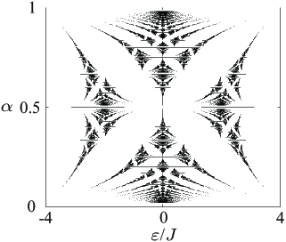
Figure 1: The Hofstadter butterfly: The eigenenergies $\epsilon$ are shown as black dots for different $\alpha$, and $J$ is the hopping energy as defined in the text. The most dominant feature is the splitting of the energy band into $r$ subbands for $\alpha=1/r$. For further details of this plot see Hofstadter .

Fractal energy band structures are believed to play an important role for a number of effects like the quantum Hall effect induced by magnetic fields in strongly correlated electron systems 2dmagn ; qhall . Therefore it is desirable to study the Hofstadter butterfly experimentally under well defined conditions. However, it turns out that the area of the elementary cells in metals where fractal energy bands could possibly be seen is so small that huge magnetic fields would be required to obtain values of $\alpha$ which are on the order of $1$ Hofstadter . Also in more sophisticated superlattice setups with larger area $A$ it is experimentally very difficult to obtain direct clear experimental evidence of the Hofstadter butterfly hofexp .

We will consider a 2D system of ultracold atoms trapped in one layer in the $xy$ plane of a three dimensional optical lattice. The atoms are in the lowest motional band which can be achieved e.g. by loading the optical lattice from a Bose-Einstein condensate bloch02 ; jaksch98 . Hopping along the $z$ direction is turned off completely by the lattice potential. Different columns of the lattice trap atoms in internal states $|g\rangle$ ($|e\rangle$) (denoted in Fig. 2a by open (closed) circles) bloch0201 ; jaksch99 . In addition the optical lattice is either accelerated along the $x$-axis or an inhomogeneous static electric field is applied and two Raman lasers driving transitions between the states $|g\rangle$ and $|e\rangle$ induce hopping along the $x$-axis while hopping along the $y$-axis is controlled by the depth of the optical lattice along this direction. This setup corresponds to applying a magnetic field with a parameter $\alpha=q\lambda/4\pi$ where $q$ is the wave number of the Raman lasers along the $y$ direction and $\lambda$ the wave length of the lasers creating the optical lattice. We also note that the atomic setup we are going to describe here can be used for a large number of other purposes. It is straightforward to add terms to the system that correspond to an external electric field. Also the atoms will interact with each other via collisional contact interactions jaksch99 and off site interactions can be engineered by dipolar Rydberg interactions jaksch00 . Therefore the setup presented here can be used for a number of studies related to the behavior of charged particles in a 2D configuration subject to magnetic and electric fields and also to study strongly interacting and thus strongly correlated systems. Furthermore it might be possible to extend this model to different geometries of optical lattices.

In this work we will concentrate on a possible setup required to implement the effective magnetic field in an optical lattice. We will discuss in detail the laser setup which leads to an effective magnetic flux through the optical lattice, and calculate the corresponding matrix elements in Sec. II. We also show that it is possible to reach each point within the Hofstadter butterfly apart from a negligibly small region around $\alpha=0$ with the proposed setup. In Sec. III we suggest one possibility of measuring some of the basic properties of the Hofstadter butterfly and discuss the limitations on the resolution for measuring the energy bands. We also give a brief account of the interaction effects. Finally we conclude with a short outlook on how the present setup could be extended in Sec. IV. While the focus of the present work is the derivation of the single-particle terms in the Hubbard Hamiltonian mimicking a strong magnetic field, we see as one of the main motivations the extension of strongly correlated many-atom systems in strong (effective) magnetic fields.

II Setup and model

In this section we discuss the experimental setup required to produce a Hofstadter butterfly for neutral atoms. We first present the optical lattice setup, then introduce an additional acceleration or static electric field and finally describe in detail the additional lasers required for our purpose.

II.1 Optical lattice

We consider a three dimensional optical lattice created by standing wave laser fields which generate a potential for the atomic motion of the form (we use $\hbar=1$ throughout the paper)

$$V(\vec{x})=V_{0x}\sin^{2}(kx)+V_{0y}\sin^{2}(ky)+V_{0z}\sin^{2}(kz),$$ (1)

with $k=2\pi/\lambda$ the wave-vector of the light and spatial coordinate ${\bf x}=\{x,y,z\}$. The recoil energy is given by $E_{R}=k^{2}/2M$ with $M$ the mass of the atoms. We assume the lattice to trap atoms in two different internal hyperfine states $|e\rangle$ and $|g\rangle$ and the depth of the lattice in $x$- and $z$-direction to be so large that hopping in these directions due to kinetic energy is prohibited jaksch98 . Furthermore we assume that adjusting the polarization of the lasers which confine the particles in the $x$-direction allows to place the potential wells trapping atoms in the different internal states at distances $\lambda/4$ with respect to each other jaksch99 ; brennen99 ; bloch0201 as shown in Fig. 1a. Therefore the resulting 2D lattice has a lattice constant (disregarding the internal state) in $x$-direction of $a_{x}=\lambda/4$ and in $y$-direction of $a_{y}=\lambda/2$. We restrict our analysis to one layer of the optical lattice in the $xy$ plane since in the following there will neither be hopping nor interactions between different layers. The dynamics of bosonic atoms occupying the lowest Bloch band of this optical lattice is well described by the Bose-Hubbard model (BHM) jaksch98

$$H_{\rm latt}=\sum_{n,m}J^{y}\left(a^{\dagger}_{n,m}a_{n,m-1}+\rm{h.c.}\right)$$

$$\quad+\sum_{n\in\text{even},m}\omega_{eg}a^{\dagger}_{n,m}a_{n,m}+\sum_{n,m}U_{n}a^{\dagger}_{n,m}a^{\dagger}_{n,m}a_{n,m}a_{n,m}$$

$$\quad+U_{x}\sum_{n,m}a^{\dagger}_{n,m}a^{\dagger}_{n+1,m}a_{n+1,m}a_{n,m},$$ (2)

where $J^{y}$ is the hopping matrix element for particles to tunnel between adjacent sites along the $y$-direction. The energy difference between the two hyperfine states is $\omega_{eg}>0$ and the operators $a_{n,m}$ ($a^{\dagger}_{n,m}$) are bosonic destruction (creation) operators for atoms in the lowest motional band located at the site which is centered at ${\bf x}_{n,m}=\{x_{n},y_{m}\}$, where $x_{n}=n\lambda/4$ and $y_{m}=m\lambda/2$. The corresponding mode functions are the localized Wannier functions $w({\bf x-\bf x}_{n,m})$ jaksch98 found by suitable superpositions of the Bloch functions for the lowest Bloch band of the lattice. Since in $x$-direction the separation between two neighboring atoms is half the original lattice constant $\lambda/2$ the overlap of the mode functions of particles in adjacent lattice sites might lead to significant nearest neighbor interactions described by $U_{x}$ whereas we neglect any other offsite interactions jaksch98 . The parameter $U_{n}$ describes the onsite interaction between two particles occupying the same site. This onsite interaction may depend on the column index $n$ because of different internal states with different scattering lengths occupying different columns. Since for even [odd] $n$ the operator $a_{n,m}$ describes atoms in internal states $|e\rangle$, [$|g\rangle$] and the Wannier functions for sites which are separated by multiples of the original lattice constant $\lambda/2$ are orthogonal to each other we find the commutation relations $[a_{n,m},a^{\dagger}_{n^{\prime},m^{\prime}}]=\delta_{n,n^{\prime}}\delta_{m,m^{\prime}}$ with $\delta_{n,n^{\prime}}$ the Kronecker delta. The details of the derivation of the above Hamiltonian can be found in jaksch98 where also the definitions for the parameters $U$, $U_{x}$, and $J^{y}$ are given.

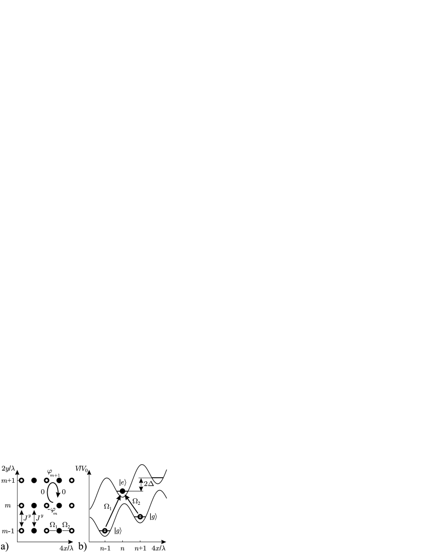
Figure 2: Optical lattice setup: Open (closed) circles denote atoms in state $|g\rangle$ ($|e\rangle$). a) Hopping in the $y$-direction is due to kinetic energy and described by the hopping matrix element $J^{y}$ being the same for particles in states $|e\rangle$ and $|g\rangle$. Along the $x$-direction hopping amplitudes are due to the additional lasers. b) Trapping potential in $x$-direction. Adjacent sites are set off by an energy $\Delta$ because of the acceleration or a static inhomogeneous electric field. The laser $\Omega_{1}$ is resonant for transitions $|g\rangle\leftrightarrow|e\rangle$ while $\Omega_{2}$ is resonant for transitions between $|e\rangle\leftrightarrow|g\rangle$ due to the offset of the lattice sites. Because of the spatial dependence of $\Omega_{1,2}$ atoms hopping around one plaquette get phase shifts of $2\pi\alpha=-\varphi_{m}+0+\varphi_{m+1}+0$ where $\varphi_{m}=mq\lambda/4\pi$ as indicated in a).

II.2 Acceleration or static electric field

In addition to the above setup we assume an energy offset of $\Delta$ between two adjacent sites in $x$-direction as shown in Fig. 2b. This can be done by accelerating the optical lattice along the $x$-axis with a constant acceleration $a_{\rm acc}$ leading to an additional potential energy term for one atom of $H_{\rm acc}=Ma_{\rm acc}x$. Alternatively, if both of the internal atomic states $|e\rangle$ and $|g\rangle$ have the same static polarizability $\mu$ an inhomogeneous static electric field of the form $E(x)=\delta Ex$ can be applied to the optical lattice yielding a potential energy term $H_{\rm acc}=\mu\delta Ex$. We keep this additional potential energy small compared to the optical lattice potential and treat $H_{\rm acc}$ as a perturbation. In second quantization this yields $H_{\rm acc}=\Delta\sum_{n,m}na^{\dagger}_{n,m}a_{n,m}$ where $\Delta=\mu\delta E\lambda/4$ in the case of an inhomogeneous electric field and $\Delta=Ma_{\rm acc}\lambda/4$ if the lattice is accelerated. The condition for this perturbative treatment to be valid is $\Delta\ll\nu_{x}$ with $\nu_{x}=\sqrt{4E_{R}V_{0x}}$ the trapping frequency of the optical lattice in the $x$-direction.

II.3 Additional lasers

Finally, we want to induce hopping along the $x$-direction by two additional lasers driving Raman transitions between the states $|g\rangle$ and $|e\rangle$. Each of them consists of two running plane waves chosen to give space dependent Rabi frequencies of the form

$$\Omega_{1,2}=\Omega e^{\pm iqy},$$ (3)

with $\Omega$ the magnitude of the Rabi frequencies, and detunings $\pm\Delta$. We choose the parameters $\Omega>0$, $\Delta>0$, and $q>0$. As discussed in detail in Appendix A this can always be achieved by superimposing two running wave laser beams incident in the $xy$-plane for $q>(\Delta+\omega_{eg})/c$ with $c$ the speed of light. We assume the lasers not to excite any higher lying motional Bloch bands and also no transitions with detunings of the order of $\Delta$, i.e., $\Omega\ll\Delta\ll\nu_{x}$. Then the lasers $\Omega_{1(2)}$ will only drive transitions $n-1\leftrightarrow n$ if $n$ is even (odd) and we can neglect any influence of the nonresonant transitions. We find the following Hamiltonian describing the effect of the additional lasers

$$H_{\rm las} = \sum_{m,n}\left(\gamma_{n,m}a^{\dagger}_{n,m}a_{n-1,m}+{\rm h.c.}\right)$$ (4)

$$\quad-\Delta\sum_{n,m}na^{\dagger}_{n,m}a_{n,m},$$

where we have neglected all other terms due to being nonresonant and defined matrix elements $\gamma_{n}$ for even $n$

$$\gamma_{n,m}=\frac{1}{2}\int d^{3}\!x\;{\bf w}^{*}({\bf x}-{\bf x}_{n,m})\Omega_{1}{\bf w}({\bf x}-{\bf x}_{n-1,m}),$$ (5)

and for odd $n$

$$\gamma_{n,m}=\frac{1}{2}\int d^{3}\!x\;{\bf w}^{*}({\bf x}-{\bf x}_{n,m})\Omega^{*}_{2}{\bf w}({\bf x}-{\bf x}_{n-1,m}).$$ (6)

For an optical lattice potential of the form Eq. (1) the Wannier functions can be written as a product of three normalized Wannier functions, i.e. ${\bf w}({\bf x})=w(x)w(y)w(z)$ jaksch98 , and we can write

$$\gamma_{n,m}=\frac{1}{2}e^{2\pi i\alpha m}\Gamma_{y}(\alpha)\Gamma_{x},$$ (7)

where we have defined the matrix elements

$$\Gamma_{x} = \int d\!x\;w^{*}(x)w(x-\lambda/4),$$

$$\Gamma_{y}(\alpha) = \int d\!y\;w^{*}(y)\cos(4\alpha\pi y/\lambda)w(y),$$ (8)

and $\alpha=q\lambda/4\pi$. The values of $\Gamma_{x}$ and $\Gamma_{y}(\alpha)$ as a function of the depth of the optical lattice $V_{0}$ are shown in Fig. 3. Both matrix elements are sufficiently large so that the above inequality $\Omega\ll\Delta\ll\nu_{x}$ can be fulfilled if we want to achieve hopping amplitudes $J^{x}=\Omega\Gamma_{x}\Gamma_{y}/2\approx J^{y}$ of the order of kHz. We simplify $H_{\rm las}$ to find

$$H_{\rm las} = \sum_{m,n}\left(J^{x}e^{2\pi i\alpha m}a^{\dagger}_{n,m}a_{n-1,m}+{\rm h.c.}\right)$$ (9)

$$\quad-\Delta\sum_{n,m}na^{\dagger}_{n,m}a_{n,m}.$$

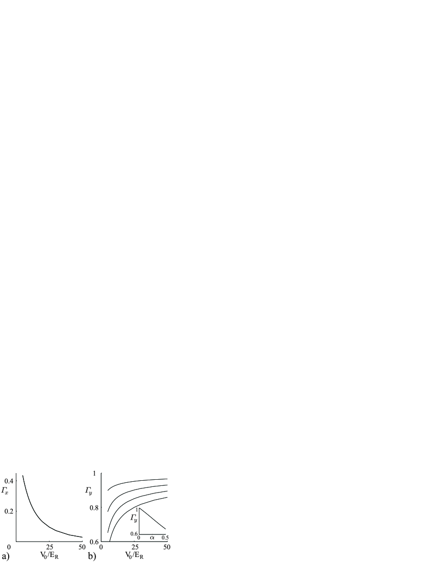
Figure 3: Matrix elements: a) $\Gamma_{x}$ as a function of the depth of the optical lattice $V_{0}/E_{R}$. b) Matrix element $\Gamma_{y}(\alpha)$ as a function of the depth of the optical lattice $V_{0}/E_{R}$ for different values of $\alpha=\{1/8,1/4,3/8,1/2\}$ decreasing with increasing $\alpha$. The inset shows $\Gamma_{y}(\alpha)$ against $\alpha$ at $V_{0}/E_{R}=10$.

II.4 Total Hamiltonian

The total Hamiltonian describing the configuration shown in Fig. 2 is given by $H=H_{\rm latt}+H_{\rm acc}+H_{\rm las}$ and we will for simplicity assume $J^{x}=J^{y}=J$. In this work we will mainly consider small filling factors of the optical lattice $\bar{n}\ll 1$ with $\bar{n}$ the average number of particles per lattice site and thus only look at one particle effects neglecting the interaction terms $U_{n}$ and $U_{x}$. Then the Hamiltonian can be written as

$$H(\alpha)=J\sum_{n,m}\left(e^{2\pi i\alpha m}a^{\dagger}_{n,m}a_{n+1,m}+a^{\dagger}_{n,m}a_{n,m+1}+{\rm h.c.}\right).$$ (10)

This Hamiltonian $H(\alpha)$ is equivalent to the Hamiltonian for electrons with charge $e$ moving on a lattice in an external magnetic field $B=2\pi\alpha/Ae$ Hofstadter , where $A=a_{x}a_{y}$ is the area of one elementary cell. In the remainder of this paper we will study the properties of $H$ for neutral atoms in optical lattices and in particular show that it can be used to study the whole of the Hofstadter butterfly shown in Fig. 1. We note that we have chosen the detunings of the additional lasers $\Omega_{1,2}$ to exactly cancel the term $H_{\rm acc}$ arising from the acceleration or electric field. If these two terms did not cancel the remaining terms resemble a homogeneous electric field.

III Discussion

In this section we show how to detect basic properties of the fractal energy spectrum in an experiment. We also briefly discuss the effects of fluctuations in the laser parameters, of finite system sizes, and interactions between the atoms.

III.1 Measurement

One way of experimentally identifying the number of energy bands in the case of rational $\alpha$ is to measure the time evolution of the particle density $\bar{n}(y,t)$ in the lattice. We assume the lattice to be loaded from a Bose-Einstein condensate bloch02 neglect any interaction between the atoms and consider only a single atom. The initial wave function of the system is assumed to be

$$|\Psi(t=0)\rangle=\frac{1}{\cal N}\sum_{n,m}a_{n,m}^{\dagger}|\text{vac}\rangle,$$ (11)

with $|\text{vac}\rangle$ the vacuum state and $\cal N$ a normalization constant. We then turn on the additional lasers to simulate a magnetic field and find the density of particles given by

$$\bar{n}(y,t)=\langle\Psi(t)|a_{n,m}^{\dagger}a_{n,m}|\Psi(t)\rangle,$$ (12)

to be independent of $x$. If we choose $\alpha=1/r$ a periodic interference pattern emerges in the time evolution of $|\Psi(t)\rangle$. Different paths for hopping around in the lattice interfere with periodic phase relations (cf. Fig. 4a). The periodicity of interference pattern is determined by $r$ and repeats itself after exactly $r$ lattice sites as can be seen in Fig. 4a for $\alpha=1/6$. The periodicity is destroyed for values of $\alpha$ which are irrational. An example can be seen in Fig. 4b where a value of $\alpha=1/2\pi$ is chosen which differs by about $5\%$ from $\alpha=1/6$. This little change in $\alpha$ is sufficient to considerably alter the density of particles in the lattice and to destroy any periodicity.

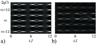
Figure 4: Particle density: $\bar{n}(y,t)$ (in arbitrary units) as a function of time $t$ and spatial coordinate $y$. Light (dark) areas indicate a large (small) particle density. a) For $\alpha=1/6$ a periodic particle density with a period of exactly $6$ lattice sites emerges. b) For a value of $\alpha=1/2\pi$ the periodicity in the particle density disappears and the visibility of the interference fringes decreases.

III.2 Parameter fluctuations

As discussed by Hofstadter Hofstadter the maximum number of energy bands shown in Fig. 1, which can in principle be distinguished in an experiment, depends on the fluctuations in the parameter $\alpha$. In our case these fluctuations are determined by the frequency stability of the lasers and will thus not be significant. In an experiment with neutral atoms the resolution of the energy bands will rather be determined by the size of the whole sample, i.e. by the number $2L/\lambda$ where $L$ is the size of the whole sample, and by the spatial resolution in measuring interference patterns as described in Sec. III.1.

III.3 Interaction effects

For large filling $\bar{n}\geq 1$ the interaction terms in the Hamiltonian Eq. 2, especially the onsite interactions become significant and cannot be neglected. We postpone a detailed study of these effects to a further publication and only include a graph of how the ground state in an optical lattice with a superimposed 2D harmonic trap of trapping frequency $\omega_{T}$

$$V(x,y)=\frac{M\omega_{T}^{2}}{2}\left(x^{2}+y^{2}\right)$$ (13)

looks like in the presence of the effective magnetic field. We use mean field theory in the form of the Gutzwiller ansatz (as described in jaksch98 ), and numerically solve for the ground state of the system for finite $U_{n}=U$ . In Fig. 5 we plot the particle number fluctuations $\sigma_{n,m}^{2}=(\langle\hat{n}_{n,m}^{2}\rangle-\langle\hat{n}_{n,m}\rangle^{2})/\langle\hat{n}_{n,m}\rangle$ with $\hat{n}_{n,m}=a^{\dagger}_{n,m}a_{n,m}$ and the modulus of the superfluid parameter $\phi_{n,m}=\langle a_{n,m}\rangle$. The effective magnetic field alters these properties of the ground state significantly in comparison to the case of $\alpha=0$. The effective magnetic field leads to a decrease of the particle number fluctuations and the superfluid density in the center of the trap which is typical for the onset of a Mott-insulating phase even for $U<U_{c}$ with $U_{c}$ the critical interaction strength for the transition to the Mott insulator. A similar behavior has already been found in monien . In addition we find from the numerics that interference effects lead to point like increase/decraese in $|\phi|$ and $\sigma$ in several of the lattice sites.

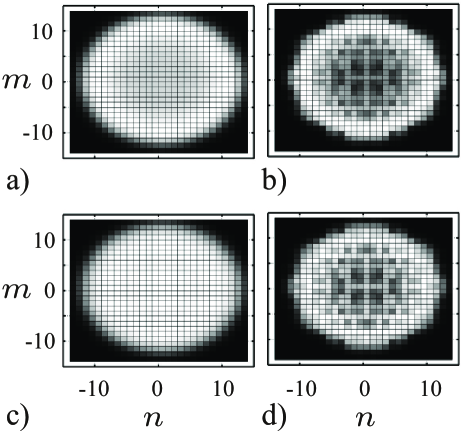
Figure 5: Ground state with interactions: Particle number fluctuations $\sigma_{n,m}$ [a), b)] and superfluid parameter $|\Phi_{n,m}|$ [c), d)] as a function of $n$ and $m$ for $U=16J<U_{c}\approx 5.8\times 4J$, $\omega_{T}=0.06J$ and chemical potential $\mu_{c}=6J$. The plots a), c) [b), d)] show the case $\alpha=0$ [$\alpha=1/6$]. Light (dark) areas indicate large (small) values of the functions (black corresponds to 0 white to 1).

IV Conclusions

In conclusion we have shown that quantum optical techniques allow to implement Hamiltonians often used to model charged particles subject to an external magnetic field in a lattice. We have shown that all of the physically interesting parameter regime can be explored by this setup and proposed one method to measure some of the most striking features of the fractal energy bands of the Hofstadter butterfly.

The setup we have investigated possesses a lot of possibilities for further extensions towards quantum simulations of strongly correlated systems of charged particles like interacting electrons moving on a lattice subject to electric and magnetic fields. The major difference and at the same time one of the most attractive features of the atomic system is a large degree of control that can be exerted by quantum optical means. In comparison to condensed matter systems the Hamiltonian describing the system is very well known and the parameters appearing can be controlled and varied over a much wider range than is usually the case for strongly correlated systems. Also, the time scale over which these parameters can be changed is short in comparison to decoherence time scales in the system. This allows to study coherent dynamical effects that are not easily accessible in most condensed matter systems. The detailed investigation of such aspects lies beyond the scope of this paper and will be dealt with in future publications.

Appendix A Laser configuration

We describe the configuration for realizing $\Omega_{1}$, the realization of $\Omega_{2}$ is then straightforward if lasers with sufficiently different frequencies to avoid interferences between $\Omega_{1}$ and $\Omega_{2}$ are used. Two running laser waves with Rabi frequencies $\Omega_{e(g)}$ and corresponding laser frequencies $\omega_{e(g)}$ for driving the transitions $|e\rangle\leftrightarrow|r\rangle$ ($|g\rangle\leftrightarrow|r\rangle$) with a large detuning $\delta_{r}$ are superimposed. We adiabatically eliminate the auxiliary internal level $|r\rangle$ and the resulting Rabi frequency for the Raman transition between $|e\rangle$ and $|g\rangle$ is then given by

$$\Omega_{1}=\frac{\Omega_{e}\Omega_{g}}{2\delta_{r}}e^{i({\bf k}_{e}-{\bf k}_{g}){\bf x}}$$ (14)

where ${\bf k}_{e(g)}=k_{e(g)}\{\cos(\phi_{e(g)}),\pm\sin(\phi_{e(g)}),0\}$ is the wave vector of the laser $\Omega_{e(g)}$. Both lasers are assumed to be incident in the $xy$ plane at angles $\phi_{e}$ and $-\phi_{g}$, respectively. If a $z$ component of the wave vectors is avoided the experiment can be done in several identically prepared planes of the lattice simultaneously which enhances the measurement signal. For a given $q=k_{e}\sin(\phi_{e})+k_{g}\sin(\phi_{g})$, $\Delta^{\prime}=(\Delta+\omega_{eg})/c=k_{g}-k_{e}$ fulfilling the requirement that $k_{e}\cos(\phi_{e})-k_{g}\cos(\phi_{g})=0$ we find

$$\cos\phi_{e}=\frac{\Gamma}{2q(k_{g}-\Delta^{\prime})},\qquad\cos\phi_{g}=\frac{\Gamma}{2qk_{g}},$$ (15)

where $\Gamma=\sqrt{(q^{2}-\Delta^{\prime 2})(4k_{g}^{2}-q^{2}-4k_{g}\Delta^{\prime}+\Delta^{\prime 2})}$. These solutions are only physically meaningful for $\Delta^{\prime}<q<\sqrt{4k_{g}(k_{g}-\Delta^{\prime})+\Delta^{\prime 2}}$. Since $\Delta^{\prime}\ll 1/\lambda$ the resulting limitations on possible values of $q$ do not constrain possible values of $\alpha$ severely. Only a negligibly small range of values of $\alpha\approx 0$ will not be realizable due to these constraints. We note that if we allow the lasers to have a $z$-component of their wave vector any value of $\alpha$ is possible.

References

- (1) M. Greiner, O. Mandel, T. Esslinger, T.W. Haensch, I. Bloch, Nature 415, 39 (2002).
- (2) O. Mandel, M. Greiner, A. Widera, T. Rom, T.W. Haensch, I. Bloch, cond-mat/0301169.
- (3) G.K. Brennen, C.M. Caves, P.S. Jessen, and I.H. Deutsch, Phys. Rev. Lett. 82, 1060 (1999); G.K. Brennen, I.H. Deutsch, and P.S. Jessen, Phys. Rev. A 61, 062309 (2000).
- (4) W. Hofstetter, J.I. Cirac, P. Zoller, E. Demler, and M. Lukin, Phys. Rev. Lett. 89, 220407 (2002).
- (5) D. Jaksch, H.-J. Briegel, J.I. Cirac, C.W. Gardiner, and P.Zoller, Phys. Rev. Lett. 82 , 1975 (1999).
- (6) D. Jaksch, J.I. Cirac, P. Zoller, S.L. Rolston, R. Cote, and M.D. Lukin, Phys. Rev. Lett. 85, 2208 (2000).
- (7) R. Raussendorf and H.-J. Briegel, Phys. Rev. Lett. 86, 5188 (2001).
- (8) U. Dorner, P. Fedichev, D. Jaksch, M. Lewenstein, and P. Zoller, quant-ph/0212039.
- (9) D. Jaksch, V. Venturi, J.I. Cirac, C.J. Williams, and P. Zoller, Phys. Rev. Lett. 89, 040402 (2002).
- (10) T. Esslinger, K. Molmer, cond-mat/0210324.
- (11) K. Molmer, Phys. Rev. Lett. 90, 110403 (2003).
- (12) A. Sorensen and K. Molmer, Phys. Rev. Lett. 83, 2274 (1999).
- (13) E. Jane, G. Vidal, W. Dür, P. Zoller, J.I. Cirac, quant-ph/0207011.
- (14) H.L. Stormer, D.C. Tsui, and A.C. Gossard, Rev. Mod. Phys. 71, S298 (1999).
- (15) For a review of quantum degenerate gaes, and in particular vortices in rotating Bose Einstein condensates see: Nature, 416, 206 (2002).
- (16) B. Paredes, P. Fedichev, J.I. Cirac, and P. Zoller, Phys. Rev. Lett. 87, 010402 (2001).
- (17) D.R. Hofstadter, Phys. Rev. B 14, 2239 (1976).
- (18) V.Y. Demikhovskii, D.V. Khomitskiy, cond-mat/0212629; M. Koshino, H. Aoki, T. Osada, K. Kuroki, and S. Kagoshima, Phys. Rev. B 65, 045310 (2002).
- (19) C. Albrecht, J.H. Smet, K. von Klitzing, D. Weiss, V. Umansky, and H. Schweizer Phys. Rev. Lett. 86, 147 (2001).
- (20) D. Jaksch, C. Bruder, J.I. Cirac, C.W. Gardiner and P. Zoller, Phys. Rev. Lett. 81, 3108 (1998).
- (21) M. Niemeyer, J.K. Freericks, and H. Monien, Phys. Rev. B 60, 2357 (1999).