Unambiguous quantum state filtering

Abstract

In this paper, we consider the generalized measurement where one particular quantum signal is unambiguously extracted from a set of non-commutative quantum signals and the other signals are filtered out. Simple expressions for the maximum detection probability and its POVM are derived. We applyl such unambiguous quantum state filtering to evaluation of the sensing of decoherence channels. The bounds of the precision limit for a given quantum state of probes and possible device implementations are discussed.

I Introduction

Discrimination of non-commutative quantum states is one of the central issues in the field of quantum information processing. Since quantum mechanics does not allow us to discriminate non-commutative states perfectly, several quantum measurement strategies have been studied for various figures of merits, such as average error probability Helstrom_QDET , mutual information Davies78 ; Sasaki99 , and success probability of unambiguous state discrimination Chefles98-1 ; Chefles98-2 ; Eldar03 ; Herzog02 ; Sun02 ; Rudolph03 . These studies have been motivated not only by academic interest, but also more technological interests from the viewpoints of quantum communication, quantum cryptography, and interferometric sensing.

In this paper, we discuss an alternative class of quantum measurement, where a signal is unambiguously extracted when it is in a particular target state, i.e., unambiguous quantum state filtering. Suppose a signal set consists of arbitrary quantum states $\hat{\rho}_{0}$ and $\hat{\rho}_{1}$, and the signals are detected by the measurement operators $\hat{\Pi}_{0}$ and $\hat{\Pi}_{1}$. We consider the measurement which maximizes the success probability of detecting $\hat{\rho}_{0}$, $P={\rm Tr\,}[\hat{\Pi}_{0}\hat{\rho}_{0}]$, under the condition that $\hat{\rho}_{1}$ never be detected incorrectly as $\hat{\rho}_{0}$, i.e., ${\rm Tr\,}[\hat{\Pi}_{0}\hat{\rho}_{1}]=0$. This is the special case of Neyman-Pearson hypothesis testing NeymanPearson33 , namely, a strategy to maximize the success probability (to follow the conventional theory, we call it the ‘detection probability’) while keeping the false-alarm probability equal to zero.

The Neyman-Pearson approach is effective for a decision problem where the prior probabilities of signals are unreliably known or unknown. Its quantum version has recently been applied to quantum interferometric sensing Paris97 ; D'Ariano02 ; Takeoka02 . The problem of the quantum Neyman-Pearson approach is, however, that the analytical solution is only known for pure state signals Helstrom_QDET . Our formulation includes mixed state signals and we show that the maximum detection probability and its corresponding detection operators are given by quite simple expressions. We also generalize the problem to the case of more than two signals. Figure 1 compares our state filtering scenario to the other measurement scenarios discussed so far. It is stressed again that the cost of our testing scenario does not include the prior probabilities of the signals. We also note that the pure state filtering scenarios with Bayesian hypothesis testing have been discussed in context of minimum-error and unambiguous discriminations of quantum signal subsets Herzog02 ; Sun02 , and the latter one was recently recasted by the more general theory of mixed state unambiguous discrimination Rudolph03 .

After discussing the formulation of unambiguous state filtering, we apply it to the sensing of quantum channels consisting of non-unitary operations as an example of applications. This scenario would be important for practical applications because various kinds of decoherence in quantum channels are described by non-unitary operators. To sense small decoherence parameters of such channels, we need to detect the mixed state probes appropriately. We discuss the detection strategy based on unambiguous state filtering and propose possible experimental implementations.

The paper is organized as follows. In Sec. II, the general formulation of the problem treated in this paper is given. In Sec. III and IV, we apply our formalism to the problem of non-unitary quantum channel sensing. As concrete examples, we consider the sensing of two practically important operations, i.e., depolarizing and linear loss in discrete and continuous variable quantum channels, respectively. Section V contains our concluding remarks.

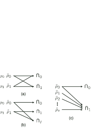
Figure 1: Various generalized quantum measurement scenarios: (a) minimum-error state discrimination, (b) unambiguous state discrimination and (c) unambiguous state filtering. Here, $p_{i}$’s in (a) and (b) are the prior probabilities of signals.

II Optimal measurement for unambiguous state filtering

In this section, we derive a rigorous formulation of the optimal measurement for our problem. We discuss first the filtering strategy for a binary signal set and then generalize it to the case of more than two signals. The generalization can be done straightforwardly.

Let us review the problem. Arbitrary quantum signals $\hat{\rho}_{0}$ and $\hat{\rho}_{1}$ are detected by the positive operator-valued measure (POVM) $\{\hat{\Pi}_{0},\,\hat{\Pi}_{1}\}$, where $\hat{\Pi}_{0}+\hat{\Pi}_{1}=\hat{I}$, and our task is to maximize the detection probability, $P={\rm Tr\,}[\hat{\Pi}_{0}\hat{\rho}_{0}]$, under the condition that ${\rm Tr\,}[\hat{\Pi}_{0}\hat{\rho}_{1}]=0$. We note that this kind of measurement is described by the Z-channel model and was first discussed by Kennedy for the detection of binary phase-shift keyed coherent signals with quasi-minimum average error probability Kennedy73 .

We denote the Hilbert spaces supporting $\hat{\rho}_{0}$ and $\hat{\rho}_{1}$ by ${\cal H}_{0}$ and ${\cal H}_{1}$, respectively, and their union by ${\cal H}={\cal H}_{0}\cup{\cal H}_{1}$. We assume that the dimensions of ${\cal H}$ and ${\cal H}_{1}$ are $n=\dim{\cal H}>0$ and $m=\dim{\cal H}_{1}>0$, respectively, where obviously $n\geq m$. Since we can limit the support spaces of $\hat{\Pi}_{0}$ and $\hat{\Pi}_{1}$ within the Hilbert space ${\cal H}$, these operators are expressed as

$$\hat{\Pi}_{0} = \sum_{k=1}^{n}\pi_{k}|\phi_{k}\rangle\langle\phi_{k}|\ ,$$ (1)

$$\hat{\Pi}_{1} = \sum_{k=1}^{n}(1-\pi_{k})|\phi_{k}\rangle\langle\phi_{k}|\ ,$$ (2)

where the set $\{|\phi_{1}\rangle,|\phi_{2}\rangle,...,|\phi_{n}\rangle\}$ is the complete orthonormal basis set in ${\cal H}$ and the positivity of detection operators requires $0\leq\pi_{k}\leq 1$ for all $k$. As a consequence, our problem is now to decide the eigenvalues $\{\pi_{k}\}$ and eigenvectors $\{|\phi_{k}\rangle\}$ of these operators.

From Eq. (1), the necessary condition for our measurement is now rewritten as

$${\rm Tr\,}[\hat{\Pi}_{0}\hat{\rho}_{1}]=\sum_{k=1}^{n}\pi_{k}\langle\phi_{k}|\hat{\rho}_{1}|\phi_{k}\rangle=0\ .$$ (3)

Since $\hat{\rho}_{1}$ is supported by the $m$-dimensional Hilbert space ${\cal H}_{1}$, its spectral decomposition is given by

$$\hat{\rho}_{1}=\sum_{\mu=1}^{m}\lambda_{\mu}|\psi_{\mu}\rangle\langle\psi_{\mu}|\ ,$$ (4)

where $\lambda_{\mu}>0$ and $\sum\lambda_{\mu}=1$ ($\mu=1,2,...,m$). The set $\{|\psi_{1}\rangle,|\psi_{2}\rangle,...,|\psi_{m}\rangle\}$ is the complete orthonormal basis set in ${\cal H}_{1}$. Equations (3) and (4) give the condition,

$$\sum_{k=1}^{n}\sum_{\mu=1}^{m}\lambda_{\mu}\pi_{k}|\langle\phi_{k}|\psi_{\mu}\rangle|^{2}=\sum_{\mu=1}^{m}\lambda_{\mu}\left(\sum_{k=1}^{n}\pi_{k}|\langle\phi_{k}|\psi_{\mu}\rangle|^{2}\right)=0\ .$$ (5)

In other words, the condition

$$\pi_{k}=0\quad{\rm or}\quad\langle\phi_{k}|\psi_{\mu}\rangle=0\ ,$$ (6)

must be satisfied for all $k$ and $\mu$ ($k=1,2,...,n;\,\mu=1,2,...,m$). Since the set $\{|\phi_{1}\rangle,|\phi_{2}\rangle,...,|\phi_{n}\rangle\}$ is complete and orthonormal in ${\cal H}={\cal H}_{0}\cup{\cal H}_{1}$, if $\langle\phi_{k}|\psi_{\mu}\rangle=0$ for all $k$, then $|\psi_{\mu}\rangle=0$, and this contradicts the assumption $m=\dim{\cal H}_{1}>0$. Eventually, there is at least one index $k_{\mu}$, such that $\pi_{k_{\mu}}=0$ for each $\mu$, that is, at least $m$ eigenvalues take a zero value,

$$\pi_{k_{1}}=\pi_{k_{2}}=...=\pi_{k_{m}}=0\ .$$ (7)

Now let us maximize the detection probability $P$,

$$P={\rm Tr\,}[\hat{\Pi}_{0}\hat{\rho}_{0}]=\sum_{k=1}^{n}\pi_{k}\langle\phi_{k}|\hat{\rho}_{0}|\phi_{k}\rangle\ .$$ (8)

Since $\langle\phi_{k}|\hat{\rho}_{0}|\phi_{k}\rangle\geq 0$, we should choose $\pi_{k}$ ($k=1,2,...,n$) to be as large as possible to maximize $P$. From Eq. (7) and $0\leq\pi_{k}\leq 1$, we find that $P$ is maximized when

$$\left\{\begin{array}[]{l}\pi_{k_{1}}=\pi_{k_{2}}=...=\pi_{k_{m}}=0,\\ \pi_{k}=1\quad(k\neq k_{1},k_{2},...,k_{m})\ ,\end{array}\right.$$ (9)

is satisfied.

Next, we derive the relation between $\{|\phi_{k}\rangle\}$ and $\{|\psi_{\mu}\rangle\}$. Let us consider the case that every index $k_{\mu}$ is not equal to each other, i.e., $\mu_{i}\neq\mu_{j}\to k_{\mu_{i}}\neq k_{\mu_{j}}$ comment1 . Since Eq. (9) means that, for each $\mu$, there is only one index $k_{\mu}$ such that $\langle\phi_{k_{\mu}}|\psi_{\mu}\rangle\neq 0$, $|\psi_{\mu}\rangle$ can be expressed as

$$|\psi_{\mu}\rangle=\sum_{k=1}^{n}g_{\mu}(k)|\phi_{k}\rangle=|\phi_{k_{\mu}}\rangle\ .$$ (10)

As a consequence, the detection operator $\hat{\Pi}_{0}$

$$\hat{\Pi}_{0} = \sum_{k=1}^{n}|\phi_{k}\rangle\langle\phi_{k}|\quad(k\neq k_{1},k_{2},...,k_{m})$$ (11)

$$= \hat{I}-\sum_{\mu=1}^{m}|\psi_{\mu}\rangle\langle\psi_{\mu}|\ .$$

Then we arrive at the optimal POVM,

$$\hat{\Pi}_{0}=\hat{I}-\sum_{\mu=1}^{m}|\psi_{\mu}\rangle\langle\psi_{\mu}|,\quad\hat{\Pi}_{1}=\sum_{\mu=1}^{m}|\psi_{\mu}\rangle\langle\psi_{\mu}|\ .$$ (12)

Apparently, if $n=m$, then $\hat{\Pi}_{0}=0$, that is, when the support of $\hat{\rho}_{0}$ is included in that of $\hat{\rho}_{1}$ (${\cal H}_{0}\subseteq{\cal H}_{1}$), unambiguous detection of $\hat{\rho}_{0}$ is impossible comment2 . On the other hand, $P=1$ can be obtained when ${\cal H}_{0}\cap{\cal H}_{1}=\emptyset$ or, equivalently, $\hat{\rho}_{0}\hat{\rho}_{1}=\hat{\rho}_{1}\hat{\rho}_{0}=0$. When we are given a pure state $\hat{\rho}_{1}=|\psi\rangle\langle\psi|$, the optimal POVM is given by

$$\hat{\Pi}_{0}=\hat{I}-|\psi\rangle\langle\psi|\quad\hat{\Pi}_{1}=|\psi\rangle\langle\psi|\ .$$ (13)

This POVM is the same as that for pure state discrimination in Takeoka02 . This means that the physical implementation scheme proposed in Takeoka02 can be applied to mixed state signals. We further discuss this issue in the later section.

Finally, let us consider the following more general problem: we are given $s+1$ quantum states, $\hat{\rho}_{0},\hat{\rho}_{1},...,\hat{\rho}_{s}$, and to find the measurement such that (1) $\hat{\rho}_{1},\hat{\rho}_{2},...,\hat{\rho}_{s}$ never be recognized as $\hat{\rho}_{0}$, and (2) the detection probability of $\hat{\rho}_{0}$ be maximized (Fig. 1(b)). For this purpose, we rewrite Eq. (12) as

$$\hat{\Pi}_{0}=\hat{I}_{{\cal H}_{0}\cup{\cal H}_{1}}-\hat{I}_{{\cal H}_{1}},\quad\hat{\Pi}_{1}=\hat{I}_{{\cal H}_{1}}\ ,$$ (14)

where $\hat{I}_{{\cal H}}$ is the identity operator defined in the Hilbert space ${\cal H}$. When we denote the support space of $\hat{\rho}_{k}$ as ${\cal H}_{k}$, Eq. (14) is easily generalized as

$$\begin{array}[]{ccl}\hat{\Pi}_{0}&=&\hat{I}_{{\cal H}_{0}\cup{\cal H}_{1}\cup{\cal H}_{2}\cup\cdot\cdot\cdot\cup{\cal H}_{s}}-\hat{I}_{{\cal H}_{1}\cup{\cal H}_{2}\cup\cdot\cdot\cdot\cup{\cal H}_{s}}\ ,\\ \hat{\Pi}_{1}&=&\hat{I}_{{\cal H}_{1}\cup{\cal H}_{2}\cup\cdot\cdot\cdot\cup{\cal H}_{s}}\ .\end{array}$$ (15)

The maximum detection probability $P$ is then given by

$$P={\rm Tr\,}[\hat{\Pi}_{0}\hat{\rho}_{0}]=1-\sum_{k=1}^{M}\langle\Psi_{k}|\hat{\rho}_{0}|\Psi_{k}\rangle,$$ (16)

where $\{|\Psi_{1}\rangle,|\Psi_{2}\rangle,...,|\Psi_{M}\rangle\}$ is the complete orthonormal vector set of the Hilbert space ${\cal H}_{1}\cup{\cal H}_{2}\cup\cdot\cdot\cdot\cup{\cal H}_{s}$.

III Application I: Sensing of depolarization in a discrete channel

In the following two sections, we apply our measurement strategy to sensing applications. One of the simplest quantum sensing scenarios can be described as follows Paris97 : A probe field, initially prepared in $\hat{\rho}_{1}$, travels through a sample in which the probe field may or may not be perturbed. A perturbation is generally described by a completely positive (CP) map ${\cal L}$. If a perturbation occurs, the probe field is then modified to $\hat{\rho}_{0}={\cal L}\,\hat{\rho}_{1}$. Eventually, we may have an unperturbed state $\hat{\rho}_{1}$ or a perturbed state $\hat{\rho}_{0}$ as output. The task is to maximize the probability that the signal will be unambiguously detected when it suffers a perturbation ${\cal L}$.

First, let us consider a discrete quantum channel consisting of an $n$-dimensional depolarizing channel ${\cal L}_{D}$ which is characterized by the depolarizing probability $p$ NielsenChuang . This example is simple and instructive to see how non-classical probes and appropriate generalized measurements enhance the detection probability. We probe the channel, in which depolarization ${\cal L}_{D}$ may or may not occur, using a pure state input $\hat{\rho}_{1}=|\psi\rangle\langle\psi|$. If depolarizing occurs, the output state is given by NielsenChuang

$$\hat{\rho}_{0}={\cal L}_{D}|\psi\rangle\langle\psi|=(1-p)|\psi\rangle\langle\psi|+\frac{p}{n}\hat{I}\ .$$ (17)

Then, following Eqs. (8) and (13), the maximum detection probability of inferring the state $\hat{\rho}_{0}$ is given by

$$P_{D}=1-\langle\psi|\left({\cal L}_{D}|\psi\rangle\langle\psi|\right)|\psi\rangle=\frac{n-1}{n}p\ ,$$ (18)

where $P_{D}$ is independent of the input quantum state.

Next, let us consider an entangled input. An arbitrary entangled state in an $n$-dimensional space is described by $|\Psi\rangle=\sum_{k}\sqrt{\lambda_{k}}|k\rangle\otimes|k\rangle$ $(k=1,2,...,n$, $\sum_{k}\lambda_{k}=1)$ and now one part of the state is incident on the channel. The maximum detection probability of inferring the state $\hat{\rho}_{0}=({\cal L}_{D}\otimes{\cal I})|\Psi\rangle\langle\Psi|$ is then given by

$$P_{D}^{\rm ent}=1-\langle\Psi|[({\cal L}_{D}\otimes{\cal I})|\Psi\rangle\langle\Psi|]|\Psi\rangle=\left(1-\frac{1}{n}\sum_{k=1}^{n}\lambda_{k}^{2}\right)p\ .$$ (19)

Here the maximum value of $P_{D}^{\rm ent}$ is obtained when $\lambda_{1}=\lambda_{2}=\cdot\cdot\cdot=\lambda_{n}=1/n$, that is, the state is maximally entangled. On the other hand, when one of $\lambda_{k}$ is 1 and the others are 0 (i.e., the state is not entangled), $P_{D}^{\rm ent}$ takes its minimum value and becomes equal to $P_{D}$ in Eq. (18). Therefore, we see that $P_{D}^{\rm ent}\geq P_{D}$ is always held, that is, entanglement always improves the detection probability. Use of an entangled input increases the Hilbert space of the output state, enhancing the overlap between $\hat{\rho}_{0}$ and $\hat{\rho}_{1}$, as has been pointed out in D'Ariano01 .

IV Application II: Sensing of linear loss in a continuous variable channel

In this section, we examine the sensing of linear loss through probing by continuous variable quantum states. Linear loss caused by coupling between the system and a vacuum environment is one of common problems of decoherence in quantum optics and quantum information processing. When we assume that a probe is in a pure state $\hat{\rho}_{1}=|\psi\rangle\langle\psi|$, such as a coherent state, squeezed state or two-mode squeezed state, the optimal POVM is given by Eq. (13). As mentioned in Section II, this is the same as that described in Takeoka02 . Therefore, the physical implementation scheme for unitary operation sensing proposed in Takeoka02 can be directly applied to this problem. The purpose of this section is to clarify the ultimate sensing limits of linear loss for concretely given probe states.

The CP map of linear loss is given by QuantumOptics

$${\cal L}_{L}=\exp\left[g\left(\hat{\cal K}_{-}-\hat{\cal K}_{0}\right)\right]\ ,$$ (20)

where $g$ is a positive parameter and the superoperators $\hat{\cal K}_{-}$ and $\hat{\cal K}_{0}$ are defined by

$$\hat{\cal K}_{-}\hat{X}=\hat{a}\hat{X}\hat{a}^{\dagger}\qquad\hat{\cal K}_{0}\hat{X}={\textstyle\frac{1}{2}}(\hat{a}\,\hat{a}^{\dagger}\hat{X}+\hat{X}\hat{a}^{\dagger}\hat{a})\ ,$$ (21)

for an arbitrary operator $\hat{X}$. Here, $\hat{a}$ and $\hat{a}^{\dagger}$ are, respectively, annihilation and creation operators. The CP map ${\cal L}_{L}$ transforms a coherent state into another coherent state with reduced complex amplitude as

$${\cal L}_{L}|\alpha\rangle\langle\beta|=E(\alpha,\beta)\,|\alpha\sqrt{T}\rangle\langle\beta\sqrt{T}|\ ,$$ (22)

where $T=\exp(-g)$ corresponds to the transmittance of the CP map and

$$E(\alpha,\beta)=\exp\left[-\frac{1}{2}(1-T)\left(|\alpha|^{2}+|\beta|^{2}-2\alpha\beta^{*}\right)\right]\ .$$ (23)

In this section, we use $R=1-T$ as a parameter of the degree of loss.

Following the previous works Paris97 ; D'Ariano02 ; Takeoka02 , we compare the ultimate sensitivities for various probes in terms of $R_{M}$, which is defined by the solution of Eq. (8) for $R$. Here, $R_{M}$ is the minimum detectable loss for a fixed detection probability $P$. This probability may be called the acceptance probability $P_{\rm ac}$ and the value of $P_{\rm ac}$ should be determined by referring to the actual experimental conditions.

IV.1 Coherent state

A simple example is that the probe field is in a coherent state $|\psi\rangle=|\alpha\rangle$. The detection probability is given by

$$P_{L}^{\rm coh} = 1-\langle\alpha|\left({\cal L}_{L}(R)|\alpha\rangle\langle\alpha|\right)|\alpha\rangle\ ,$$ (24)

$$= 1-\exp\left[-\left|\left(1-\sqrt{1-R}\right)\alpha\right|^{2}\right]\ .$$

Then we find $R_{M}$ as

$$R_{M}^{\rm coh}=\frac{1}{\sqrt{\langle n\rangle}}\sqrt{\log\frac{1}{1-P_{\rm ac}}}\left(2-\frac{1}{\sqrt{\langle n\rangle}}\sqrt{\log\frac{1}{1-P_{\rm ac}}}\right)\ ,$$ (25)

where $\langle n\rangle=|\alpha|^{2}$ is the average photon number of the probe field. We can easily find that $R_{M}^{\rm coh}$ is proportional to $1/\sqrt{\langle n\rangle}$ within the limit of large $\langle n\rangle$, which is the same as in the case of sensing unitary operations described in Paris97 ; Takeoka02 . On the other hand, when $\langle n\rangle$ is small, $\langle n\rangle$ has to satisfy

$$\langle n\rangle\geq\langle n\rangle_{\rm min}=\log\frac{1}{1-P_{\rm ac}}\ ,$$ (26)

since $R_{M}\leq 1$. This is different from that for the sensing of unitary operations. Here, $\langle n\rangle_{\rm min}$ is the minimum required power for sensing. In other words, $\langle n\rangle_{\rm min}$ is the average power required to unambiguously detect the signal with detection probability $P_{\rm ac}$, when $|\psi\rangle$ is mapped to a vacuum state.

IV.2 Squeezed state

As a second example let us consider the squeezed state $|\psi\rangle=D(\alpha)S(\zeta)|0\rangle$ as a probe field where $\zeta=re^{i\theta}$ is the complex squeezing parameter. After tedious calculation, we get the detection probability

$$P_{L}^{\rm sq} = 1-\langle\psi|\left({\cal L}_{L}|\psi\rangle\langle\psi|\right)|\psi\rangle$$

$$= 1-\frac{1}{\sqrt{1+|\nu|^{2}R(2-R)}}\exp\left[-\frac{(1-\sqrt{1-R})^{2}}{1+|\nu|^{2}R(2-R)}\left\{|\alpha|^{2}+(2-R)\left(|\nu|^{2}|\alpha|^{2}+\frac{1}{2}\mu(\nu^{*}\alpha^{2}+\nu\alpha^{*2})\right)\right\}\right]\ ,$$

where

$$\mu=\cosh r,\quad\nu=e^{i\theta}\sinh r\ .$$ (28)

Obviously, Eq. (IV.2) depends on the phases of the coherent amplitude and squeezing. To maximize $P_{L}^{\rm sq}$, these factors should be optimized. Labeling the phase of the coherent amplitude as $\alpha=|\alpha|e^{i\varphi}$, we easily find that Eq. (IV.2) is maximized when $2\varphi-\theta=0$ is held. Now we can take $\varphi=\theta=0$ (amplitude squeezing) without loss of generality. Then Eq. (IV.2) is simplified to

$$P_{L}^{\rm sq}=1-\frac{1}{\sqrt{1+\sinh^{2}r\,R(2-R)}}\exp\left[-\frac{(1-\sqrt{1-R})^{2}}{1+\sinh^{2}r\,R(2-R)}(1-e^{-r}\sinh r\,R)e^{2r}\alpha^{2}\right]\ .$$ (29)

In the following, we apply the power constraint condition, $\langle n\rangle=\bar{n}+\bar{m}$, where $\langle n\rangle$ is the total average number of photons, $\bar{n}=|\alpha|^{2}$ and $\bar{m}=\sinh^{2}r$. In Fig. 2, $R_{M}^{\rm sq}$ with $P_{\rm ac}=1/2$ for a given $\langle n\rangle$ is plotted with $\bar{m}=0$ (coherent state), $\bar{m}=0.2\langle n\rangle$, $\bar{m}=0.9\langle n\rangle$, and $\bar{m}=\langle n\rangle$ (squeezed vacuum). This figure shows that the optimal power distribution to $\bar{n}$ and $\bar{m}$ depends on the total power $\langle n\rangle$ of the probe field.

Before further considering the optimization of power distribution for a squeezed input, we give analytical expressions for some limited cases. When the power for the probe field is fully used for squeezing ($\bar{m}=\langle n\rangle$), i.e., the probe is in a squeezed vacuum state, $P_{L}$ is simply given by

$$P_{L}^{\rm sv}=1-\frac{1}{\sqrt{1+\langle n\rangle R(2-R)}}\ .$$ (30)

Then we find $R_{M}$ and the minimum required power as

$$R_{M}^{\rm sv}=1-\sqrt{1-\frac{1}{\langle n\rangle}\left\{\left(\frac{1}{1-P_{\rm ac}}\right)^{2}-1\right\}}\ ,$$ (31)

and

$$\langle n\rangle_{\rm min}=\left(\frac{1}{1-P_{\rm ac}}\right)^{2}-1\ ,$$ (32)

respectively. Within the limit of large $\langle n\rangle$, $R_{M}^{\rm sv}$ is approximately proportional to $\langle n\rangle$ as

$$R_{M}^{\rm sv}\approx\frac{1}{2\langle n\rangle}\left\{\left(\frac{1}{1-P_{\rm ac}}\right)^{2}-1\right\}\ .$$ (33)

On the other hand, when we assume $\bar{n}\gg\bar{m}$, which is important from a practical point of view, Eq. (29) can be approximated to

$$P_{L}^{\rm sq}\approx 1-\exp\left[-(1-\sqrt{1-R})^{2}e^{2r}\alpha^{2}\right]\ ,$$ (34)

and then

$$R_{M}^{\rm sq}\approx\frac{1}{e^{r}\sqrt{\bar{n}}}\sqrt{\log\frac{1}{1-P_{\rm ac}}}\left(2-\frac{1}{e^{r}\sqrt{\bar{n}}}\sqrt{\log\frac{1}{1-P_{\rm ac}}}\right)\ ,$$ (35)

which shows that a bright squeezed probe field improves the minimum detectable loss by a factor of $e^{r}$.

Figure 3 shows $R_{M}^{\rm opt}$ with $P_{\rm ac}=1/2$, where the power distribution for squeezing is numerically optimized. For reference, the optimal power ratio $\bar{m}/\langle n\rangle$ and the ratio between $R_{M}^{\rm opt}$ and $R_{M}^{\rm sv}$ are plotted in the same figure. We found that $R_{M}^{\rm opt}$ asymptotically reached about 92% of $R_{M}^{\rm sv}$, which means that $R_{M}^{\rm opt}$ is also proportional to $\langle n\rangle$ within the limit of large $\langle n\rangle$. The minimum required power is about $\langle n\rangle_{\rm min}=0.60$, which is slightly better than that of coherent state probing ($\langle n\rangle_{\rm min}=0.69$).

Figure 2: Minimum detectable loss $R_{M}$ as a function of total photon number $\langle n\rangle$. $\bar{m}=\sinh^{2}r$ is a function of the squeezing parameter $r$. $P_{\rm ac}=1/2$.

Figure 3: Minimum detectable loss $R_{M}$ for the squeezed probe in which the power distribution to $\bar{n}$ and $\bar{m}$ are optimized. For reference, the corresponding power distribution $\bar{m}/\langle n\rangle$ and the ratio of $R_{M}$ between the optimized squeezed probe and the squeezed vacuum probe are plotted. $P_{\rm ac}=1/2$.

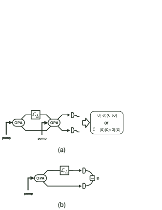
Figure 4: Sensing of linear loss by a two-mode squeezed vacuum probe and (a) optimal measurement or (b) measurement of the photon number difference.

IV.3 Two-mode squeezed vacuum

Our final example is a probe field consisting of the two-mode squeezed vacuum state,

$$|\Psi\rangle=\sqrt{1-\lambda^{2}}\sum_{n=0}^{\infty}\lambda^{n}|n\rangle|n\rangle\ ,$$ (36)

where $\lambda=\tanh r$ and we assume that the squeezing parameter $r$ is real and positive without loss of generality. Let us consider the sensing scheme in which one part of the two-mode squeezed vacuum state is incident on a tested channel and then all of the output modes are measured collectively. The optimal POVM is described by $\{\hat{\Pi}_{0}=\hat{I}-|\Psi\rangle\langle\Psi|,\,\hat{\Pi}_{1}=|\Psi\rangle\langle\Psi|\}$ and thus we obtain the detection probability as

$$P_{L}^{\rm tmsv} = 1-\langle\Psi|\left[\left({\cal L}_{L}\otimes{\cal I}\right)|\Psi\rangle\langle\Psi|\right]|\Psi\rangle$$ (37)

$$= 1-\left(\frac{1-\lambda^{2}}{1-\lambda^{2}\sqrt{1-R}}\right)^{2}\ .$$

Note that this measurement can be physically implemented through the same strategy as used by Takeoka02 , for example, through a system consisting of parametric three-wave mixing and photo-detection to discriminate between zero and non-zero photons, as shown in Fig. 4(a). From Eq. (37), we find $R_{M}$ as

$$R_{M}^{\rm tmsv} = \frac{1}{\langle n\rangle}\left(\frac{1}{\sqrt{1-P_{\rm ac}}}-1\right)$$ (38)

$$\times\,\left\{2-\frac{1}{\langle n\rangle}\left(\frac{1}{\sqrt{1-P_{\rm ac}}}-1\right)\right\}\ ,$$

where the minimum required power is

$$\langle n\rangle_{\rm min}=\frac{1}{\sqrt{1-P_{\rm ac}}}-1\ .$$ (39)

Here, $\langle n\rangle=\lambda^{2}/(1-\lambda^{2})$ is the average power incident on a tested channel. Obviously, within the limit of large $\langle n\rangle$, $R_{M}^{\rm tmsv}$ is almost proportional to $1/\langle n\rangle$.

Finally, we briefly discuss another strategy that is based on measurement of the photon number (photocurrent) difference, which works effectively in some interferometric schemes using entanglement D'Ariano02 . The schematic is shown in Fig. 4(b). Here the state is discriminated by observing whether the difference in the photon number between two photo-detectors is zero or non-zero, i.e., by the set of measurement operators $\{\hat{\Pi}_{0}=\hat{I}-\sum_{n}|n\rangle|n\rangle\langle n|\langle n|,\,\hat{\Pi}_{1}=\sum_{n}|n\rangle|n\rangle\langle n|\langle n|\}$. Although this is not optimal since the support space of $\sum_{n}|n\rangle|n\rangle\langle n|\langle n|$ is obviously larger than that of Eq. (36), to find the precision limit of this simpler measurement scheme is still interesting from a practical point of view. The detection probability is calculated to be

$$P_{L}^{\rm tmsv} = 1-\sum_{n=0}^{\infty}\langle n|\langle n|\left[\left({\cal L}_{L}\otimes{\cal I}\right)|\Psi\rangle\langle\Psi|\right]|n\rangle|n\rangle$$ (40)

$$= 1-\frac{1-\lambda^{2}}{1-\lambda^{2}(1-R)}\ ,$$

and we find the minimum detectable loss and the minimum required power as

$$R_{M}^{\rm tmsv}=\frac{1}{\langle n\rangle}\left(\frac{P_{\rm ac}}{1-P_{\rm ac}}\right)\ ,$$ (41)

and

$$\langle n\rangle_{\rm min}=\frac{P_{\rm ac}}{1-P_{\rm ac}}\ ,$$ (42)

respectively.

To summarize, we plotted the $R_{M}$’s for coherent, squeezed, and two-mode squeezed probes with $P_{\rm ac}=1/2$ in Fig. 5. Again, a two-mode squeezed (entangled) probe showed better performance than single-mode squeezed probes. Since the total power for a probe is defined by the power incident on a tested channel only, the expansion of the output Hilbert space due to an entangled probe clearly enables greater sensitivity. Fortunately, we can also see that when the input power is sufficiently larger than $\langle n\rangle_{\rm min}$, the strategy of detecting the photon number difference is near optimal. This strategy may be simpler than the optimal one in regions of large $\langle n\rangle$ where currently available photodetectors can operate. However, an entangled probe provides the most drastic gain in regions where the input power is extremely limited, when it is measured by the optimal measurement scheme.

Figure 5: Minimum detectable loss $R_{M}$ for various probe fields.

V Concluding remarks

In this paper, we have discussed the measurment scenario of unambiguous quantum state filtering where one particular signal is unambiguously extracted from a set of non-orthogonal signals. The maximum detection probability and its corresponding measurement operators are given by simple expressions although our formulation includes mixed state signals.

As an application, we have considered the sensing of decoherence in quantum channels. We applied this formalism to the sensing of two kinds of decoherence channels, a depolarizing channel and a channel which included linear loss. A probe field is initially in a pure state and the output is probably in a mixed state. The latter channel is especially important in practice since we often encounter such decoherence in optical quantum communication networks. Our results suggest that the asymptotic behavior of the precision limit is the same as that of unitary operation sensing, for example, phase shift sensing Paris97 ; D'Ariano02 ; Takeoka02 . On the other hand, in the region of a weak probe field, for probes to have non-zero detection probabilities there are minimum required powers. These results show how a non-classical, especially an entangled, probe and an appropriate detection scheme improve sensing performance.

References

• (1) C. W. Helstrom, Quantum Detection and Estimation Theory (Academic Press, New York, 1976).
• (2) E. B. Davies, IEEE Trans. Inf. Theory IT-24, 596 (1978).
• (3) M. Sasaki, S. M. Barnett, R. Jozsa, M. Osaki, and O. Hirota, Phys. Rev. A 59, 3325 (1999).
• (4) A. Chefles, Phys. Lett. A 239, 339 (1998).
• (5) A. Chefles and S. M. Barnett, Phys. Lett. A 250, 223 (1998).
• (6) Y. C. Eldar, IEEE Trans. Inf. Theory IT-49, 446 (2003).
• (7) U. Herzog and J. A. Bergou, Phys. Rev. A 65, 050305(R) (2002).
• (8) Y. Sun, J. A. Bergou, and M. Hillery, Phys. Rev. A 66, 032315 (2002).
• (9) T. Rudolph, R. W. Spekkens, and P. S. Turner, LANL arXive quant-ph/0303071 (2003).
• (10) J. Neyman and E. Pearson, Philos. Trans. R. Soc. London, Ser. A 231, 289 (1933).
• (11) M. G. A. Paris, Phys. Lett. A 225, 23 (1997).
• (12) G. M. D’Ariano, M. G. A. Paris, and P. Perinotti, Phys. Rev. A 65, 062106 (2002).
• (13) M. Takeoka, M. Ban, and M. Sasaki, LANL arXive quant-ph/0212037 (2002).
• (14) R. S. Kennedy, Research Laboratory of Electronics, MIT, Quarterly Progress Report No. 108, 219 (1973).
• (15) Suppose $k_{\mu_{1}}=k_{\mu_{2}}\,(\equiv k_{0})$. It induces $\langle\phi_{k_{0}}|\psi_{\mu_{1}}\rangle=\langle\phi_{k_{0}}|\psi_{\mu_{2}}\rangle\neq 0$ and $\langle\phi_{k}|\psi_{\mu_{1}}\rangle=\langle\phi_{k}|\psi_{\mu_{2}}\rangle=0$ ($k\neq k_{0}$), eventually, $|\psi_{\mu_{1}}\rangle=|\psi_{\mu_{2}}\rangle=|\phi_{k_{0}}\rangle$. Since $\{|\psi_{1}\rangle,|\psi_{2}\rangle,...,|\psi_{m}\rangle\}$ is the set of eigenvectors of $\hat{\rho}_{1}$, the above statement is in contradiction to the assumption that $\hat{\rho_{1}}$ is supported by the $m$-dimensional Hilbert space ${\cal H}_{1}$.
• (16) For example, although it is possible to construct the filtering measurement which extracts the thermal state unambiguously from a signal set consisting of a thermal state and a vacuum state, its converse (extraction of the vacuum state) is impossible.
• (17) M. A. Nielsen and I. L. Chuang, Quantum Computation and Quantum Information (Cambridge University Press, Cambridge, 2000).
• (18) G. M. D’Ariano, P. LoPresti, and M. G. A. Paris, Phys. Rev. Lett. 87, 270404 (2001).
• (19) D. F. Walls and G. J. Milburn, Quantum Optics (Springer-Verlag, Berlin, 1994).