Measurement induced entanglement and quantum computation with atoms in optical cavities

Abstract

We propose a method to prepare entangled states and implement quantum computation with atoms in optical cavities. The internal state of the atoms are entangled by a measurement of the phase of light transmitted through the cavity. By repeated measurements an entangled state is created with certainty, and this entanglement can be used to implement gates on qubits which are stored in different internal degrees of freedom of the atoms. This method, based on measurement induced dynamics, has a higher fidelity than schemes making use of controlled unitary dynamics.

An essential ingredient in the construction of a quantum computer is the ability to entangle the qubits in the computer. In most proposals for quantum computation this entanglement is created by a controlled interaction between the quantum systems which store the quantum information fortschritte . An alternative strategy to create entanglement is to perform a measurement which projects the system into an entangled state cabrillo ; brian , and based on this principle a quantum computer using linear optics, single photon sources, and single photon detectors has recently been proposed linear . Here we present a similar proposal for measurement induced entanglement and quantum computation on atoms in optical cavities, which only uses coherent light sources and homodyne detection, and we show that high fidelity operation can be achieved with much weaker requirements for the cavity and atomic parameters than in schemes which rely on a controlled interaction.

Several schemes for measurement induced entanglement have been proposed for atoms in optical cavities bose ; plenio ; hong ; duan ; plenioto , but compared to these schemes our proposal has the advantage that entanglement can be produced with certainty even in situations with finite detector efficiency. Furthermore, our procedures are similar to methods already in use to monitor atoms in cavities hood , and we therefore believe that the current proposal should be simpler to implement. Indeed the atom counting procedure in the experiment in Ref. mckeever could be sufficient to implement this scheme.

We consider atoms with two stable ground states $|g\rangle$ and $|f\rangle$ and an excited state $|e\rangle$ as shown in Fig. 1 (a). Both atoms are initially prepared in an equal superposition of the two ground states, $(|g\rangle+|f\rangle)/\sqrt{2}$. By performing a Quantum Non-Demolition (QND) measurement which measures $N$, the number of atoms in state $|f\rangle$, the state vector is projected into the maximally entangled state $|\Psi_{{\rm EPR}}\rangle=(|gf\rangle+|fg\rangle)/\sqrt{2}$ provided we get the outcome $N=1$. If the outcomes $N=0$ or $N=2$ are achieved, the resulting state is $|gg\rangle$ or $|ff\rangle$, so that the initial state can be prepared once again, and we can repeat the QND-measurement until the desired entangled state is produced. On average two measurements suffice to produce the state. With $M$ atoms in the cavity, the scheme can be extended to the generation of multiparticle entangled states where the population of the $|f\rangle$ state is distributed symmetrically on all atoms. If, e.g., $M=3$ we may produce with certainty the W-states w-state $(|ffg\rangle+|fgf\rangle+|gff\rangle)/\sqrt{3}$ by performing the detection $4/3$ times on average. Also, one could entangle a small subset of the atoms by leaving all other atoms in $|g\rangle$ so that they do not contribute to $N$.

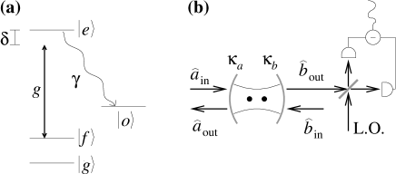
Figure 1: Energy levels and experimental setup of the atoms. (a) The atoms have two groundstates $|g\rangle$ and $|f\rangle$, and the cavity couples the state $|f\rangle$ to the excited state $|e\rangle$ with coupling strength $g$ and detuning $\delta$. The excited state $|e\rangle$ decays to an auxiliary state $|o\rangle$ with a decay rate $\gamma$. (b) Two atoms are located inside a cavity and light is shined into the cavity in the mode described by $\hat{a}_{{\rm in}}$. After mixing with a local oscillator (L.O.), the transmitted light is measured by homodyne detection.

The implementation of the QND detection is a modification of a scheme presented in Ref. reflection where QND detection was achieved by measuring single photons reflected from a cavity. To generate entangled states with a high fidelity this method is undesirable because it is very sensitive to imperfections in the cavity and to imperfect mode matching. Instead we propose to measure the light transmitted through the cavity with homodyne detection. The proposed experimental setup is shown in Fig. 1 (b). The atoms are trapped inside the cavity, and we consider a single field mode described by the annihilation operator $\hat{c}$. Photons in the cavity can decay through two leaky mirrors with decay rates $\kappa_{a}$ and $\kappa_{b}$, and the incoming and outgoing fields at the mirror with decay rate $\kappa_{a}$ ($\kappa_{b}$) are described by $\hat{a}_{{\rm in}}$ and $\hat{a}_{{\rm out}}$ ($\hat{b}_{{\rm in}}$ and $\hat{b}_{{\rm out}}$). Light is shined into the cavity in the $\hat{a}_{{\rm in}}$ mode, and the transmitted light in the $\hat{b}_{{\rm out}}$ mode is measured by balanced homodyne detection. In the cavity the light couples the state $|f\rangle$ of the $k$th atom to the excited state $|e\rangle$ with a coupling constant $g_{k}$. We mainly consider light far from resonance with the atoms, where the interaction changes the phase of the field by an angle proportional to $N$. By measuring the phase of the transmitted light with homodyne detection, we thus obtain the desired QND detection of $N$. Spontaneous emission from the excited state limits the amount of light we can send through the cavity, and below we evaluate the fidelity $F$, obtainable for a given set of cavity parameters ($F=\langle\Psi_{{\rm EPR}}|\rho|\Psi_{{\rm EPR}}\rangle$, where $\rho$ is the atomic density matrix). The excited state $|e\rangle$ decays with a rate $\gamma$, and for simplicity we assume that the atoms end up in some other state $|o\rangle$ after the decay. Because these states have a vanishing overlap with the desired state our results will lead to a lower fidelity than if we had assumed that the atoms decay back to the state $|f\rangle$, but it does not affect the scaling with cavity parameters, which is our main interest here.

The interaction of the cavity light with the atoms is described by the Hamiltonian

$$H=\sum_{k}g_{k}|e\rangle\langle f|_{k}\hat{c}+g_{k}^{*}\hat{c}^{\dagger}|f\rangle\langle e|_{k}+\delta|e\rangle\langle e|_{k},$$ (1)

where $\delta$ is the detuning of the atoms from the cavity resonance, and where the sum is over all atoms in the cavity. The decay of the $k$th atom is described by a Lindblad relaxation operator $d_{k}=\sqrt{\gamma}|o\rangle\langle e|_{k}$, and the input/output relations are given by $d\hat{c}/dt=-i[\hat{c},H]-(\kappa/2)\hat{c}+\sqrt{\kappa_{a}}\hat{a}_{{\rm in}}+\sqrt{\kappa_{b}}\hat{b}_{{\rm in}}+\sqrt{\kappa^{\prime}}\hat{F}$, $\hat{a}_{{\rm out}}=\hat{a}_{{\rm in}}-\sqrt{\kappa_{a}}\hat{c}$, and $\hat{b}_{{\rm out}}=\hat{b}_{{\rm in}}-\sqrt{\kappa_{b}}\hat{c}$, where $\kappa=\kappa_{a}+\kappa_{b}+\kappa^{\prime}$ is the total decay rate, and $\kappa^{\prime}$ and $\hat{F}$ is the decay rate and noise operator associated with cavity loss to other modes than the two modes considered. For convenience $\hat{c}$ has the standard normalization for a single mode $[\hat{c},\hat{c}^{\dagger}]=1$, whereas the normalization for the free fields are such that, e.g., $[\hat{a}_{{\rm in}}(t),\hat{a}_{{\rm in}}(t^{\prime})^{\dagger}]=\delta(t-t^{\prime})$. We assume that the atoms are separated by more than the resonant optical wavelength, and we hence ignore the dipole-dipole interaction between the atoms. We solve the equations of motion by assuming that the fields are sufficiently weak that only the lowest order terms in $\hat{c}$ are important. Note that this limits the total number of photon in the cavity at any time, but the total number of photons in a pulse may still be large. By taking the Fourier transform we find the cavity field to be given by reflection

$$\hat{c}(\omega)=\frac{\sqrt{\kappa_{a}}\hat{a}_{{\rm in}}(\omega)}{\frac{\kappa}{2}-i\omega+\frac{g^{2}\hat{N}}{\gamma/2+i(\delta-\omega)}}+{\rm noise},$$ (2)

where we have introduced the operator $\hat{N}=\sum_{k}|f\rangle\langle f|_{k}(t=0)$ which counts the number of atoms in state $|f\rangle$ before the pulse, and we have assumed that the magnitude of all coupling constants are identical $|g_{k}|^{2}=g^{2}$. Using Eq. (2) we find an expression for the transmitted light

$$\hat{b}_{{\rm out}}(\omega)=\frac{-\sqrt{\kappa_{a}\kappa_{b}}}{\frac{\kappa}{2}-i\omega+\frac{g^{2}\hat{N}}{\gamma/2+i(\delta-\omega)}}\hat{a}_{{\rm in}}(\omega)+{\rm noise}.$$ (3)

We determine the Heisenberg equations of motion for the atoms from Eq. (1) and the relaxation operators and solve them by assuming that the atomic ground state operators vary only little on the time scale $1/\gamma$. Here we shall only need the projection operator onto the $|f\rangle$ state, which after the interaction with the light pulse $(t=\infty)$ is given by $|f\rangle\langle f|(t=\infty)=:|f\rangle\langle f|(t=0)\exp(-\hat{\theta}):$, where $:\quad:$ denotes normal ordering, and where we have introduced the scattering probability operator

$$\hat{\theta}=\gamma\int d\omega\frac{g^{2}}{\frac{\gamma^{2}}{4}+(\delta-\omega)^{2}}\hat{c}(\omega)^{\dagger}\hat{c}(\omega).$$ (4)

The incoming light is assumed to be in a coherent state with frequency $\omega$ and since Eq. (3) is linear the outgoing field will also be in a coherent state $|\beta_{N}\rangle$. Using Eqs. (2)-(4) we see that the difference between the coherent state output of an empty cavity and that of a cavity with $N$ atoms can be expressed as

$$|\beta_{N}-\beta_{0}|^{2}=N^{2}\frac{g^{2}\kappa_{b}}{\gamma(\frac{\kappa^{2}}{4}+\omega^{2})}\theta_{N},$$ (5)

The scattering probability per atom $\theta_{N}$ [obtained by inserting Eq. (2) in Eq. (4)] depends on the number of atoms, because the field amplitude inside the cavity depends on $N$. From Eq. (5) we see that the best signal to noise ratio ($|\beta_{N}-\beta_{0}|^{2}/\theta_{N}$) is obtained by use of light which is resonant with the cavity, $\omega=0$. For resonant light, the transmittance of the output mirror should match all other losses $\kappa_{b}=\kappa_{a}+\kappa^{\prime}=\kappa/2$, and the QND detection then only depends on the cavity parameters through the combination $g^{2}/\kappa\gamma$. In particular, $|\beta_{N}-\beta_{0}|^{2}=N^{2}\theta_{N}g^{2}/\kappa\gamma$. If $\kappa_{b}$ deviates from $\kappa/2$ the effective $g^{2}/\kappa\gamma$ is changed by $2\kappa_{b}/\kappa$. If transmitted photons are lost, or if they are only detected with a probability $\eta$, the effective $g^{2}/\kappa\gamma$ is reduced by this factor.

If we need to distinguish an empty cavity from a cavity with a certain number of atoms, the signal to noise ratio is independent of the detuning of the cavity from the atomic resonance, but here we concentrate on the far detuned case $\delta\gg g^{2}/\kappa$, $\gamma$, where the $N=1$ and $N=2$ components are easier to distinguish. In this limit the intra cavity field and therefore the scattering probability $\theta_{N}$ is independent of $N$ and we replace $\theta_{N}$ by the same $\theta$ for all $N$. If the light is on resonance with the cavity $\omega=0$, and far detuned from the atomic resonance, we see from Eq. (3) that the interaction with the atoms changes the phase of the field by an angle proportional to $N$. By adjusting the phase of the local oscillator we can configure the measurement so that the photocurrent difference, integrated over the duration of the pulse, can be normalized to a dimensionless field quadrature operator $x$ which, in turn, is proportional to the phase change imposed by the atoms and, hence, it provides a QND detection of $N$. If the atoms are in the $N=0$ state, light is transmitted through the cavity without being affected by the atoms, and the homodyne measurement provides a value for $x$ in accordance with a Gaussian probability distribution $p_{0}(x)=\exp(-x^{2})/\sqrt{\pi}$ with a variance $(\Delta x)^{2}=1/2$ due to vacuum noise in the coherent state. If $N=1$ or 2, Eq. (5) predicts the Gaussian to be displaced so that it is centered around $x_{N}=2N\sqrt{\theta g^{2}/\kappa\gamma}$.

So far we have ignored that the atoms are slowly pumped out of the state $|f\rangle$ due to decay of the upper state, and this changes the distribution. If we start with $N$ atoms in state $|f\rangle$, the probability distribution $p_{N}(x)$ can be written as a sum of a part $p_{{\rm ND},N}(x)$ where there has been no atomic decay and a part $p_{{\rm D},N}(x)$ where at least one of the atoms have decayed: $p_{N}(x)=p_{{\rm ND},N}(x)+p_{{\rm D},N}(x)$. With no decay Eq. (5) is valid and we have $p_{{\rm ND},N}(x)=\exp(-N\theta)p_{0}(x-x_{N})$. If there is a decay, Eq. (3) is valid until the time of the decay and we find $p_{{\rm D},1}=\int_{0}^{\theta}d\theta^{\prime}\exp(-\theta^{\prime})p_{0}(x-x_{1}\theta^{\prime}/\theta)$ and $p_{{\rm D},2}=2\int_{0}^{\theta}d\theta^{\prime}\exp(-\theta-\theta^{\prime})p_{0}(x-x_{1}(\theta^{\prime}+\theta)/\theta)+\int_{0}^{\theta}d\theta^{\prime}\int_{0}^{\theta}d\theta^{\prime\prime}\exp(-\theta^{\prime}-\theta^{\prime\prime})p_{0}(x-x_{1}(\theta^{\prime}+\theta^{\prime\prime})/\theta)$. If the homodyne measurement produces an outcome $\tilde{x}$ in a region $x_{a}<\tilde{x}<x_{b}$ around $x_{1}$, the atoms are most likely in the desired entangled state and the measurement is successful. The probability for this measurement outcome is $P_{s}=\int_{x_{a}}^{x_{b}}d\tilde{x}P_{\rm tot}(\tilde{x})$, where the total probability distribution for $\tilde{x}$ is given by $P_{{\rm tot}}(\tilde{x})=p_{0}(\tilde{x})/4+p_{1}(\tilde{x})/2+p_{2}(\tilde{x})/4$.

Figure 2: Fidelity of the produced entangled state. Starting from below, the full curves shows the obtainable error probability $1-F$ for $P_{s}=0.1\%$, 30% and 50%. The dashed curve is an upper bound on the total error probability when the scheme is repeated until it is successful.

The fidelity of the entangled state vanishes if one of the atoms has decayed to a different subspace, and the fidelity of the state produced is therefore given by the conditional probability of starting in the state with $N=1$ and not having decayed. By averaging over the interval of accepted values we get the fidelity, $F=\int_{x_{a}}^{x_{b}}d\tilde{x}p_{{\rm ND},1}(\tilde{x})/2/P_{s}$.

For a given value of $g^{2}/\kappa\gamma$ the success probability and fidelity depend on $\theta$, $x_{a}$ and $x_{b}$. To get a high fidelity one must choose a small interval around $x_{1}$ because it minimizes the contribution from $p_{0}$ and $p_{2}$, but a small interval also reduces the success probability. In Fig. 2 we show the smallest error probability $1-F$ achievable as a function of $g^{2}/\kappa\gamma$, when we vary $x_{a}$ and $\theta$ and adjust $x_{b}$ to retain a fixed value of $P_{s}$. In the figure the full curves show $1-F$ for $P_{s}=0.1\%$, $P_{s}=30\%$ and $P_{s}=50\%$.

In Fig. 2 we observe that the fidelity scales as

$$1-F\sim\frac{\kappa\gamma}{g^{2}}\log{\left(\frac{g^{2}}{\kappa\gamma}\right)}.$$ (6)

This behavior can be understood from Eq. (5): with a fixed distance $|\beta_{1}-\beta_{0}|=\sqrt{2}x_{1}$, the error due to scattering decreases as $\kappa\gamma/g^{2}$, but due to the overlap of the Gaussians there is a probability of accepting a wrong value for $N$, which will dominate over the error due to scattering if we keep the distance fixed and increase $g^{2}/\kappa\gamma$. Because the overlap of the Gaussians decreases exponentially with the square of the distance, optimum fidelity is obtained if the distance grows logarithmically with $g^{2}/\kappa\gamma$ and this gives the scaling in Eq. (6).

The scaling (6) is valid up to a success rate $P_{s}=50\%$, where $P_{{\rm tot}}(\tilde{x})$ consists of three well separated Gaussians, so that even when the scheme is not successful we know in which state ($N=0$ or $N=2$) the atoms are left. From these states we can deterministically produce the initial product state, and we can repeat the measurement procedure until it is successful. A lower limit on the fidelity with this procedure can be shown to be $F>\int_{x_{a}}^{x_{b}}d\tilde{x}p_{{\rm ND},1}(\tilde{x})/2/(1-\int_{-\infty}^{x_{a}}d\tilde{x}p_{0}(\tilde{x})/4-\int_{x_{b}}^{\infty}d\tilde{x}p_{{\rm ND},2}(\tilde{x})/4)$. This lower limit is shown with a dashed line in Fig. 2, and the scaling still follows (6).

The deterministic entanglement scheme can be used to implement gates between qubits. Suppose that the levels $|f\rangle$ and $|g\rangle$ are both degenerate with two substates. For convenience the four states $|g_{0}\rangle,\ |g_{1}\rangle,\ |f_{0}\rangle,\ |f_{1}\rangle$ can be described as tensor products of the ’level’ degree of freedom ($|g\rangle$ and $|f\rangle$) and ’qubit’ degree of freedom ($|0\rangle$ and $|1\rangle$). (This would be the natural representation if $|0\rangle$ and $|1\rangle$ represent, e.g., different motional state, but they may also be different internal states in the atoms, e.g., states with different magnetic quantum numbers). The qubits are initially stored in the states $|g_{0}\rangle$ and $|g_{1}\rangle$ and, we assume that the interactions during the entanglement preparation are symmetric with respect to the qubit degrees of freedom, so that the qubits are decoupled from the preparation of the entangled state of the levels, i.e, we prepare the state $|\Phi_{q}\rangle\otimes(|gf\rangle+|fg\rangle)/\sqrt{2}$, where $|\Phi_{q}\rangle$ is the initial state of the qubits. The entanglement in the levels $|f\rangle$ and $|g\rangle$ can now be used to implement a control-not operation on the qubits as discussed in Ref. cnot : we interchange states $|f_{1}\rangle$ and $|g_{1}\rangle$ in the control atom, and then measure if this atom is in the $|f\rangle$ or the $|g\rangle$ level. If the measurement outcome is $|g\rangle$ ($|f\rangle$) the target atom is known to be in $|g\rangle$ ($|f\rangle$) if the control atom is in $|1\rangle$, and the control-not operation amounts to interchanging the states $|g_{0}\rangle$ and $|g_{1}\rangle$ ($|f_{0}\rangle$ and $|f_{1}\rangle$) in the target atom. To complete the gate a $\pi/2$ pulse is applied between the levels $|f\rangle$ and $|g\rangle$, and a QND-measurement of the level of the target atom, followed by single atom transitions, conditioned on the outcome of the measurement leaves the system in $|\tilde{\Phi}_{q}\rangle\otimes|gg\rangle$, where $|\tilde{\Phi}_{q}\rangle$ is the desired outcome of the control-not operation on $|\Phi_{q}\rangle$. The single atom measurements required for the gate operation can be done by homodyne detection of light transmitted through the cavity, and the procedure is accomplished with a fidelity scaling as in Eq. (6).

A different strategy for quantum computation in optical cavities is to construct a controlled interaction between the atoms and the cavity field pellizzari ; domokos ; zheng : If an atom emits a photon into the cavity mode this photon can be absorbed by another atom, and this constitutes an interaction which can be used to engineer quantum gates. With controlled interactions, a first estimate of the error probability $\epsilon$ in a single gate is given by $\epsilon\sim\mathrm{max}\{\gamma,\kappa\}/g$, but this can be improved by use of Raman transitions or a large detuning between the atoms and the cavity mode. If the optical transition is replaced by a Raman transition where a classical beam with Rabi frequency $\Omega$ and detuning $\Delta$ induces a transition between two ground states and the simultaneous creation/annihilation of a photon in the cavity, the effective coupling constant is $g_{{\rm eff}}\sim g\Omega/\Delta$ and the effective decay rate is $\gamma_{{\rm eff}}\sim\gamma\Omega^{2}/\Delta^{2}$. By decreasing $\Omega/\Delta$ we can thus reduce the error probability $\gamma_{{\rm eff}}/g_{{\rm eff}}$ due to spontaneous emission. Similarly it has also been proposed to reduce the effect of cavity decay by using transitions which are detuned from the cavity zheng . If the Raman transitions are detuned by an amount $\delta$ from the cavity mode the effective coupling constant between the atoms is $\chi\sim g_{{\rm eff}}^{2}/\delta$ and the leakage rate is $\kappa_{{\rm eff}}\sim\kappa g_{{\rm eff}}^{2}/\delta^{2}$, so that the leakage can be reduced by making $\delta\gg\kappa$. But, detuning from the cavity mode increases the effect of spontaneous emission because the gate takes longer time. Since the gate duration is $t\sim 1/\chi$ the probability for spontaneous emission is $\epsilon_{\gamma}\sim\gamma\delta/g^{2}$ and the probability for a cavity decay is $\epsilon_{\kappa}\sim\kappa/\delta$. The minimum error probability $1-F=\epsilon_{\gamma}+\epsilon_{\kappa}$ is then found to scale as

$$1-F\sim\sqrt{\frac{\kappa\gamma}{g^{2}}}.$$ (7)

Although Eq. (7) has been derived for a particular setup, we believe the scaling in Eq. (7) is characteristic for all existing proposals which use a controlled interaction between the atoms. (Also the scheme in the Ref. beige has the scaling (7) if the photodetectors have finite efficiency, or if the scheme is required to implement gates deterministically). The fundamental problem is that the atomic decay and the cavity loss provide two sources of errors which combine to give the scaling in Eq. (7). For a given cavity, i.e., for given parameters $g$, $\kappa$, and $\gamma$, we obtain the better scaling presented in Eq. (6) by using a scheme where classical light is injected into the cavity and where leakage of a single photon is not a critical event.

In conclusion, we have presented a scheme to entangle atoms and implement gates between qubits which are stored in the atoms. The error probability scales more favorably than it does in schemes which use controlled interactions and unitary dynamics, and the present scheme is therefore advantageous if a high fidelity is required. The best optical cavities currently reach $g^{2}/\kappa\gamma\sim 100$ hood so that Eq. (7) predicts $F\sim 90\%$ which is less than the value in Fig. 2. More importantly, to decrease the error rate in the measurement induced scheme, e.g., by a given factor we only need to improve the cavity finesse, which is proportional to $g^{2}/\kappa\gamma$, by the same factor. With the scaling in Eq. (7) the cavity finesse should be increased by the same factor squared.

This work was supported by the Danish Natural Science Research Council and by the Natural Science Foundation through its grant to ITAMP.

References

- (1) Fortschr. Phys., 48, 765-1140 (2000) (Special issue on Experimental proposals for quantum computation).
- (2) C. Cabrillo et al., Phys. Rev. A 59, 1025 (1999).
- (3) B. Julsgaard, A. Kozhekin, and E.S. Polzik, Nature 413, 400 (2001).
- (4) E. Knill, R. Laflamme, and G. Milburn, Nature 409, 46 (2001).
- (5) S. Bose et al., Phys. Rev. Lett. 83, 5158 (1999).
- (6) M.B. Plenio et al., Phys. Rev. A 59 2468 (1999).
- (7) J. Hong and H.-W. Lee, Phys. Rev. Lett. 89, 237901 (2002).
- (8) L.M. Duan and H.J. Kimble, quant-ph/0301164.
- (9) M.B. Plenio, D.E. Browne, and S.F. Huelga, quant-ph/0302185.
- (10) C.J. Hood et al., Phys. Rev. Lett. 80, 4157 (1998).
- (11) J. McKeever et al., Phys. Rev. Lett. 90, 133602 (2003).
- (12) W. Dür, G. Vidal, and J.I. Cirac, Phys. Rev. A 62, 062314 (2000); W. Dür, Phys. Rev. A 63, 020303 (2001).
- (13) A.S. Sørensen and K. Mølmer, Phys. Rev. Lett. 90, 127903 (2003).
- (14) A. Sørensen and K. Mølmer, Phys. Rev. A 58, 2745 (1998).
- (15) T. Pellizzari et al., Phys. Rev. Lett. 75, 3788 (1995).
- (16) P. Domokos et al., Phys. Rev. A 52, 3554 (1995).
- (17) S.-B. Zheng and G.-C. Guo, Phys. Rev. Lett. 85, 2392 (2000).
- (18) A. Beige et al., Phys. Rev. Lett. 85, 1762 (2000).