Experimental Demonstration of Quantum Lattice Gas Computation

Abstract

We report an ensemble nuclear magnetic resonance (NMR) implementation of a quantum lattice gas algorithm for the diffusion equation. The algorithm employs an array of quantum information processors sharing classical information, a novel architecture referred to as a type-II quantum computer. This concrete implementation provides a test example from which to probe the strengths and limitations of this new computation paradigm. The NMR experiment consists of encoding a mass density onto an array of 16 two-qubit quantum information processors and then following the computation through 7 time steps of the algorithm. The results show good agreement with the analytic solution for diffusive dynamics. We also describe numerical simulations of the NMR implementation. The simulations aid in determining sources of experimental errors, and they help define the limits of the implementation.

I Introduction

The advent of fast quantum algorithmsGenQCRefs has spawned a broad search for new algorithms that utilize the novel features of quantum information. Among the new proposals are quantum lattice gas (QLG) algorithms, which, in analogy to their classical counterparts, make use of arrays of interacting sites to perform useful calculations. In the quantum case, however, the sites behave quantum mechanically, while the site-to-site interactions can be either classicalYepezLatticegas or quantum mechanicalMeyer_QLGA . New algorithms have been devised to solve selected computational problems such as the diffusion equationYepezDiffusion ; Meyer-Diff and the Schrödinger equationQLG-Schrodinger . In the case where the quantum mechanical sites (or nodes) communicate with each other classically, the required architecture for QLG algorithms has been termed a type-II quantum computerYepezTypeII .

A type-II device is essentially a classically parallel computer, with the exception that the computing elements follow the rules of quantum mechanics. The advantage gained from the classical network is completely analogous to the improvement gained in a classical, massively-parallel architecture. However, the use of quantum mechanical nodes introduces several notable differences. Classical lattice gas algorithms become unstable (and unusable) when the relevant transport coefficient is reduced or when nonlinearities are increased. In the quantum case, the transport coefficient and degree of nonlinearity can be varied at will using the appropriate quantum operations at each site. In addition, the quantum algorithms typically require a smaller number of qubits per site than do the classical algorithms. Finally, the family of QLG algorithms can handle increasingly complex calculations as the number of (qu)bits per site is increased. For example, when two qubits are present in a site, the QLG algorithms can solve the relatively simple diffusion equation in one, two, or three dimensions YepezDiffusion and the more difficult nonlinear Burgers equation in one dimension YepezBurgers . With four qubits per site, the QLG algorithms can solve coupled nonlinear field equations governing the velocity and magnetic fields of one-dimensional magnetohydrodynamic turbulence YepezMHD . With six qubits per site, the QLG algorithms can model the nonlinear Navier-Stokes equations in two dimensions governing a viscous fluid yepez-lncs99 . A more complete description of type-II quantum computers and their scaling properties has been given by Jeffrey Yepez YepezBurgers YepezMHD .

Here, we present a methodology for implementing a quantum lattice gas algorithm on a nuclear magnetic resonance (NMR)NMR type-II architecture. In this implementation, we encode a discrete mass density onto distinct spatial locations of a liquid-state sample. We use magnetic field gradients to discriminate between locations in the sample, thus creating an array of addressable ensemble NMR quantum information processors. In addition, we use radio frequency (RF) pulses and methods learned from previous workNMRQIPBasics1 ; NMRQIPBasics2 to execute the necessary operations in each quantum processor. The result is a concrete implementation examining the necessary control for realizing a quantum lattice-gas algorithm using NMR techniques.

II Lattice Gas Algorithms

The lattice gas method is a tool of computational physics used to model hydrodynamical flows that are too large for a standard low-level molecular dynamics treatment and that contain discontinuous interfacial boundaries that prevent a high-level partial differential equations descriptionLGOrigins1 ; LGOrigins2 ; LGOrigins3 ; LGOrigins4 . The basic idea underlying the lattice gas method is to statistically represent a macroscopic scale time-dependent field quantities by “averaging” over repeated instances of a system of artificial microscopic particles scattering and propagating throughout a lattice of interconnected sites. A particular instance of the system has many particles distributed over the lattice sites. Multiple particles may coexist at each site at a given time, and each particle carries a unit mass and a unit momentum of energy. Particles interact on site via an artificial collision rule which exactly conserves the total mass, momentum, and energy at that site. The movement of particles along the lattice is prescribed by a streaming operation that shifts particles to nearest neighboring sites, thus endowing the particles with the property of momentum. The lattice gas algorithm encapsulates the microscopic scale kinematics of the particles scattering on site and moving along the lattice. The mean-free path length between collisions is about one lattice cell size and the mean-free time between collision elapses after a single update. This is computationally simple in comparison to molecular dynamics where many thousands of updates are required to capture such particle interactions.

The mesoscopic evolution is obtained by taking the ensemble average over many instances of microscopic realizations. At the mesoscopic scale, the average presence of each particle type is defined by an occupation probability. In addition, the microscopic collision and streaming rules translate into the language of kinetic theoryKinTheory1 ; KinTheory2 ; KinTheory3 . The behavior of the system is described by a transport equation for the occupation probabilities, and this equation is a discrete Boltzmann equation called the lattice Boltzmann equation LatBoltz1 ; LatBoltz2 ; LatBoltz3 .

The lattice Boltzmann equation further translates into a macroscopic, continuous, effective field theory by letting the cell size approach zero (the limit of infinite lattice resolution called the continuum limit). At the macroscopic scale, partial differential equations describe the evolution of the field, admitting solutions such as propagating sound wave modes and diffusive modes. The passage of the Boltzmann equation to the effective field theory begins by expanding the occupation probabilities, which have a well-defined statistical functional form, in terms of the continuous macroscopic variables, such as the mass density $\rho$ (and the velocity or energy field if they are defined in the model). This expansion usually is carried out perturbatively in a small parameter such as the Knudsen number (ratio of mean-free path to the largest characteristic length scale) or the Mach number (ratio of the sound speed to the largest characteristic flow speed) in a fashion analogous to the Chapman-Enskog expansion of kinetic theory ChapEn1 ; ChapEn2 ; ChapEn3 . Conversely, and self-consistently, the macroscopic field quantities can also be expressed as a function of the mesoscopic occupation probabilities–for example, the mass density at some point is a sum over the occupation probabilities in that vicinity.

Quantum lattice gas algorithms are generalizations of the classical lattice gas algorithms described above where quantum bits are used to encode the occupation probabilities and where the principle of quantum mechanical superposition is added to the artificial microscopic world. In this quantum case, the mesoscopic occupation probabilities are mapped onto the wave functions of quantum mechanical sites. In the case where the quantum lattice gas describes a hydrodynamic system when the time evolution of the flow field is required, we must periodically measure these occupation probabilities and the quantum lattice gas algorithm becomes suited to a type-II implementation. Such type-II algorithms have been shown to solve dynamical equations such as the diffusion equation YepezDiffusion , the Burgers equation YepezBurgers , and magnetohydrodynamic Burgers turbulence YepezMHD . As a first exploration of a type-II architecture using NMR, we implemented a QLG model of diffusive dynamics in one dimension.

III Solving the 1-D Diffusion Equation

The quantum lattice gas algorithm that solves the 1-D diffusion equation derives from a classical lattice gas of particles moving up and down a 1-D latticeYepezDiffusion . The motion of the particles occurs in discrete steps (streaming phase), and the particles have a probability of changing directions (collision). When the collisions are such that the particles reverse directions half of the time, then the continuum effective field theory that emerges obeys diffusive dynamics. In this case, the motion of an individual particle is a random walk, and an arbitrary initial distribution of particles will diffuse isotropically as a function of time.

The lattice gas described above is summarized by the Boltzmann equation

$$f_{1,2}(z\pm\Delta z,t+\Delta t)=f_{1,2}(z,t)+\Omega_{1,2}(z,t),$$ (1)

where the left-hand side denotes the occupation of the lattice as a function of the previous lattice configuration and where the collision term is

$$\Omega_{1,2}=\pm\frac{1}{2}\left[f_{1}\left(1-f_{2}\right)-f_{2}\left(1-f_{1}\right)\right]$$ (2)

The variables $f_{1}\equiv f_{1}(z,t)$ and $f_{2}\equiv f_{2}(z,t)$ are the occupation probabilities for finding upward- and downward-moving particles, respectively, at the site location $z$ and time $t$. The time step is denoted by $\Delta t$, while the lattice spacing is given by $\Delta z$. The collision term changes the direction of some particles, and it is responsible for the diffusive behavior.

The interesting macroscopic quantity of the lattice gas is the mass density field, $\rho$, defined as the sum of upward- and downward-moving particles

$$\rho(z,t)=f_{1}(z,t)+f_{2}(z,t).$$ (3)

The ambiguity in assigning the mass density between the two occupation probabilities is resolved by a constraint for local equilibrium demanding that the mass density be initially distributed equally

$$f^{\hbox{\tiny eq}}_{1}(n,0)=f^{\hbox{\tiny eq}}_{2}(n,0)=\frac{1}{2}\rho(n\Delta z,0).$$ (4)

After a single time step, the occupation probabilities $f_{1}$ and $f_{2}$ evolve according to (1), resulting in a new mass density

$$\rho(z,t+\Delta t)=\frac{1}{2}\left[\rho(z+\Delta z,t)+\rho(z-\Delta z,t)\right].$$ (5)

The first finite-difference in time of the mass density field is then written as

$$\rho(z,t+\Delta t)-\rho(z,t)=\frac{1}{2}\left[\rho(z+\Delta z,t)-2\rho(z,t)+\rho(z-\Delta z,t)\right].$$ (6)

In the limit where the lattice cell size and the time step approach zero ($\Delta z\rightarrow 0$ and $\Delta t\rightarrow 0$), the mass density field becomes continuous and differentiable. The second-order Taylor expansion of equation (6) about $z$ and $t$ can thus be written in the differential form

$$\frac{\partial\rho(z,t)}{\partial t}=\left(\frac{\Delta z^{2}}{2\Delta t}\right)\frac{\partial^{2}\rho(z,t)}{\partial z^{2}}$$ (7)

where it is now evident that $\rho$ evolves according to the diffusion equation with a constant transport coefficient $\frac{\Delta z^{2}}{2\Delta t}$.

Finally, in this implementation we consider an initial mass density ${\rho(z,t=0)}$ whose evolution obeys the periodic boundary condition $\rho(z,t)=\rho(z+L,t)$, where $L$ is the length of the lattice. As a result, the initial mass density diffuses until the total mass is evenly dispersed throughout the lattice.

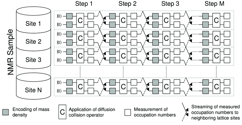
Figure 1: The circuit diagram shows the quantum lattice gas algorithm for solving the 1-D diffusion equation. The algorithm employs $N$ two-qubit sites to encode the discretized mass density. Each site codes for a single value of the mass density using the quantum state of the two qubits. The encoded information is subjected to a series of local transformations that evolve the system. The collision operator $C$ is the only potentially entangling operation in the algorithm, and it creates quantum coherences limited to each two-qubit system. The streaming is executed by classical communication, and it moves the occupation numbers up and down the lattice as denoted by the arrows. The sectioned cylinder depicts the position of the adjacent sites in the NMR sample. Each site is physically realized as an addressable slice of isotopically-labeled Chloroform solution.

The corresponding quantum lattice gas algorithm description begins by encoding the occupation probabilities, and thus the mass density, in the states of a lattice of quantum objects. The streaming and collision operations are then a combination of classical and quantum operations, including measurements. The aim of the algorithm is to take an initial mass density field and to evolve its underlying occupation probabilities according to the Boltzmann equation (1). A schematic of the entire quantum algorithm is shown in Fig. 1. A single time step of the algorithm is decomposed into four sequential operations:

1. encoding of the mass density

2. application of the collision operator $\hat{C}$ at all sites

3. measurement of the occupation numbers

4. streaming to neighboring sites.

These operations are repeated until the mass density field has evolved for the desired number of time steps. In the first time step, the encoding operation specifies the initial mass density profile, while in all the subsequent steps the encoding writes the results of the previous streaming operation. The final time step ends with the readout of the desired result, so operation 4 is not performed.

Each occupation probability is represented as the quantum mechanical expectation value of finding a two-level system, or qubit, in its excited state $|{1}\rangle$. As a result, the state of the qubit encoding the value $f_{a}(z,t)$ is

$$|{f_{a}(z,t)}\rangle=\sqrt{f_{a}(z,t)}|{1}\rangle+\sqrt{1-f_{a}(z,t)}|{0}\rangle.$$ (8)

It follows that a single value of the mass density is recorded in two qubits, one for each occupation number. The combined two-qubit wave function for a single node becomes

$$|\psi(z,t)\rangle = \sqrt{f_{1}f_{2}}|11\rangle+\sqrt{f_{1}(1-f_{2})}|10\rangle+$$

$$\sqrt{(1-f_{1})f_{2}}|01\rangle+\sqrt{(1-f_{1})(1-f_{2})}|00\rangle.$$

The kets $|00\rangle$, $|01\rangle$, $|10\rangle$, and $|11\rangle$ span the joint Hilbert space of the two qubits, and this is the largest dimension space over which quantum superpositions are allowed. As with the classical algorithm, the constraint for local equilibrium (4) forces the initial occupation probabilities at a node to be half of the corresponding mass density value.

The occupation numbers encoded in the two-qubit wave function $|\psi(z,t)\rangle$ can be recovered by measuring the expectation value of the number operator $\hat{n}_{a}$, as given in

$$f_{a}(z,t)=\langle\psi(z,t)|{\hat{n}_{a}}|\psi(z,t)\rangle,$$ (10)

where $\hat{n}_{1}=\hat{n}\otimes{\bf 1}$, $\hat{n}_{2}={\bf 1}\otimes\hat{n}$, where ${\bf 1}$ is the $2\times 2$ identity matrix, and where the action of the single-qubit number operator $\hat{n}$ returns $1$ if qubit is in its excited state and $0$ for the ground state.

The encoded occupation probabilities evolve as specified by the Boltzmann equation by the combined action of the collision operator, the measurement, and streaming. The collision operator contributes by taking the local average of the two occupation probabilities. This averaging (not to be confused with statistical coarse-grain averaging, time averaging, or ensemble averaging) is done by choosing the the collision operator $\hat{C}$ to be the “square-root of swap” gate, written as

$$\hat{C}=\left(\begin{array}[]{cccc}1&0&0&0\\ 0&\frac{1}{2}+\frac{i}{2}&\frac{1}{2}-\frac{i}{2}&0\\ 0&\frac{1}{2}-\frac{i}{2}&\frac{1}{2}+\frac{i}{2}&0\\ 0&0&0&1\end{array}\right)$$ (11)

in the standard basis. The same collision is applied simultaneously at every site, resulting in

$$|\psi^{\prime}(z,t)\rangle=\hat{C}|\psi(z,t)\rangle.$$ (12)

Using (10), the intermediate occupation probabilities of the wave function $|\psi^{\prime}(z,t)\rangle$ are

$$f_{a}^{\prime}(z,t)=\frac{1}{2}\left(f_{1}+f_{2}\right)$$ (13)

as required for $a=1,2$. The third operation physically measures these intermediate occupation probabilities $f_{a}^{\prime}(z,t)$ at all the sites. If the algorithm is performed on individual quantum systems, then the values are obtained by averaging over many strong quantum measurements of identical instances of each step. However, when the algorithm is performed using a sufficiently large ensemble of quantum systems, as in the case of NMR, then a single weak measurement of the entire ensemble can provide sufficient precision to obtain $f_{a}^{\prime}(z,t)$. A single time step is completed with the streaming of the occupation probabilities to the nearest neighbors, according to the rule

$$f_{1}(z-\Delta z,t+\Delta t)=f_{1}^{\prime}(z,t)$$ (14)

$$f_{2}(z+\Delta z,t+\Delta t)=f_{2}^{\prime}(z,t)$$ (15)

The information on the two qubits is shifted to the neighboring sites in opposite directions. The streaming operation is a classical step causing global data shifting, and it is carried out in a classical computer interfaced to the quantum processors. Together, the last three operations result in

$$f_{1,2}(z\pm\Delta z,t+\Delta t)=\frac{1}{2}\left[f_{1}(z,t)+f_{2}(z,t)\right]$$

which is the exact dynamics described by the Boltzmann equation (1).

IV NMR Implementation

IV.1 Spin System and Control

The goal of the NMR implementation is to experimentally explore the steps outlined by the diffusion QLG algorithm. For this two-qubit problem, we chose a room-temperature solution of isotopically-labeled chloroform (¹³CHCl₃), where the hydrogen nucleus and the labeled carbon nucleus served as qubits 1 and 2, respectivelyChloroRef . The chloroform sample was divided into 16 classically-connected sites of two qubits each, creating an accessible Hilbert space larger than would be available with 32 non-interacting qubits.

The internal Hamiltonian of this system in a strong and homogeneous magnetic field $B_{0}$ is

$$H_{internal}=-\frac{1}{2}\left(\gamma_{H}B_{0}\right)\sigma^{1}_{z}-\frac{1}{2}\left(\gamma_{C}B_{0}\right)\sigma^{2}_{z}+\frac{\pi J}{2}\sigma^{1}_{z}\sigma^{2}_{z}$$ (17)

where the first two terms represent the Zeeman couplings of the spins with $B_{0}$ and the last term is the scalar coupling between the two spins. The operators of the form $\sigma^{a}_{k}$ are Pauli spin operators for the spin $a$ and the Cartesian direction $k$. The choice of chloroform is particularly convenient because the different gyromagnetic ratios, $\gamma_{H}$ and $\gamma_{C}$, generate widely spaced resonant frequencies. As a result, a RF pulse applied on resonance with one of the spins does not rotate, to a very good approximation, the other spin. In the 7 T magnet utilized for the implementation, the hydrogen and carbon frequencies were about 300 MHz and 75 MHz, respectively. The widely spaced frequencies allow us to write the two RF control Hamiltonians as acting on the two spins independently. The externally-controlled RF Hamiltonians are written as

$$H_{RF}^{a}(t) = -\frac{1}{2}\left[w^{a}_{x}(t)\sigma^{a}_{x}+w^{a}_{y}(t)\sigma^{a}_{y}\right].$$ (18)

The RF Hamiltonians generate arbitrary single-spin rotations with high fidelity when the total nutation frequencies

$$\nu^{a}_{RF}=\frac{1}{2\pi}\sqrt{[w^{a}_{x}]^{2}+[w^{a}_{y}]^{2}}$$ (19)

are much stronger than $J$, the scalar coupling constant. The scalar coupling Hamiltonian and the single-spin rotations permit the implementation of a universal set of gates, and they are the building blocks for constructing more involved gates such as the collision operator $\hat{C}$NMRQIPBasics1 ; NMRQIPBasics2 .

The lattice of quantum information processors is realized by superimposing a linear magnetic field gradient on the main field $B_{0}$, adding a position dependent term to the Hamiltonian having the form

$$H_{gradient}(z)=-\frac{1}{2}\left(\gamma_{H}\frac{\partial B_{z}}{\partial z}z\right)\sigma^{1}_{z}-\\ \frac{1}{2}\left(\gamma_{C}\frac{\partial B_{z}}{\partial z}z\right)\sigma^{2}_{z}.$$ (20)

The variable $z$ denotes the spatial location along the direction of the main field, while the constant $\frac{\partial B_{z}}{\partial z}$ specifies the strength of the gradient. The usefulness of this Hamiltonian can be appreciated by noticing that the offset frequencies $\Delta\Omega_{H,C}=\gamma_{H,C}\left(\frac{\partial B_{z}}{\partial z}\right)z$ of the spins vary with position when the gradient field is applied. Spins at distinct locations can thus be addressed with RF fields oscillating at the corresponding frequencies. In this way, the magnetic field gradient allows the entire spin ensemble to be sliced into a lattice of smaller, individually addressable sub-ensembles.

Using the coupling, RF, and gradient Hamiltonians described above, together with the appropriate measurement and processing tools, we can now describe in detail how the four steps of the diffusion QLG algorithm translate to experimental tasks. The lattice initialization step (1) uses the magnetic field gradients to establish sub-ensembles of varying resonant frequency addressable with the RF Hamiltonians. The collision step (2) makes use of both the RF and the internal coupling Hamiltonians to generate the desired unitary operation $\hat{C}$NMRQIPBasics1 ; NMRQIPBasics2 . The readout (3) is accomplished by measuring the spins in the presence of a magnetic field gradient. And finally, the streaming operation (4) is performed as a processing step in a classical computer in conjunction with the next initialization step.

IV.2 Lattice Initialization

The initialization of the lattice begins by transforming the equilibrium state of the ensemble into a starting state amenable for quantum computation. At thermal equilibrium, the density matrix is

$$\sigma_{thermal}=\text{exp}\left[-\frac{H_{internal}}{k_{B}T}\right]\approx\frac{\mathbf{1}}{2^{2}}+\epsilon\left[\frac{\gamma_{H}}{\gamma_{C}}\sigma^{1}_{z}+\sigma^{2}_{z}\right]$$ (21)

where $\epsilon$ has a value on the order of $10^{-5}$. The equilibrium state is highly mixed and the two spins have unequal magnetizations. To perform quantum computations, it is convenient to transform the equilibrium state into a pseudo-pure state CoryPP ; IkePP , a mixed state whose deviation part transforms identically to the corresponding pure state and, when measured, returns expectation values proportional to those that would be obtained by measuring the underlying pure state. Two transformations create the starting pseudo-pure state $|00\rangle$ from the thermal state. First, the magnetizations of the two spins are equalized,

$$\sigma_{thermal}\stackrel{{\scriptstyle Equalize}}{{\longrightarrow}}\sigma_{equal}=\\ \frac{\mathbf{1}}{2^{2}}+\frac{\epsilon}{2}\left(1+\frac{\gamma_{H}}{\gamma_{C}}\right)\left[\sigma^{1}_{z}+\sigma^{2}_{z}\right]$$ (22)

followed by a pseudo-pure state creation sequence that results in

$$\sigma_{equal}\stackrel{{\scriptstyle Pseudo-pure}}{{\longrightarrow}}\sigma_{pp}=\\ \frac{\mathbf{1}}{2^{2}}+\epsilon\frac{\sqrt{3}}{4\sqrt{2}}\left(1+\frac{\gamma_{H}}{\gamma_{C}}\right)\\ \left[\sigma^{1}_{z}+\sigma^{2}_{z}+\sigma^{1}_{z}\sigma^{2}_{z}\right].$$ (23)

The equalization and pseudo-pure state creation sequences are described in detail in reference PPEqual . For clarity, we define the constant in front of the brackets to be $\epsilon^{\prime}$, allowing us to write the pseudopure state $\sigma_{pp}$ in terms of the desired spinor $|00\rangle$ as

$$\sigma_{pp}=\left(\frac{1}{4}-\epsilon^{\prime}\right){\mathbf{1}}+\epsilon^{\prime}|00\rangle\langle 00|.$$ (24)

Expressed in this manner, it is now seen that a unitary transformation applied to $\sigma_{pp}$ acts trivially on the term proportional to the identity, but it evolves the term $|00\rangle\langle 00|$ as it would a pure state.

Individually addressing the sites of the lattice, as depicted in Fig. 1, is accomplished by selectively addressing adjacent slices of the cylindrical sample. The procedure is related to slice-selection in magnetic resonance imaging (MRI)MRSliceSelection , and it works by applying the gradient Hamiltonian in the presence of suitably shaped RF pulses. First, consider the Hamiltonian for a one-spin system subjected to a linear magnetic field gradient in the $z$-direction and to a time-dependent RF pulse applied in the $y$-direction. In this case, the Hamiltonian is

$$H_{RF,G}(z,t)=-\frac{1}{2}\left(\gamma\frac{\partial B_{z}}{\partial z}z\right)\sigma_{z}\\ -\frac{1}{2}w_{y}(t)\sigma_{y}$$ (25)

where the $\sigma_{z}$ term is the linearly-varying static field and the $\sigma_{y}$ term is the time-dependent RF. The Hamiltonian $H_{RF,G}(z,t)$ does not commute with itself at all times, so a closed-form and exact solution cannot be easily given without specifying the function $w_{y}(t)$. A valuable approach, however, is to consider the approximate evolution generated by $H_{RF,G}(z,t)$ during infinitesimal periods of the RF pulse. To first order, the evolution during the initial period $\Delta t$ becomes

$$U_{RF,G}(z,t=\Delta t)\approx\text{exp}\left[i\frac{1}{2}\left(\gamma\frac{\partial B_{z}}{\partial z}\Delta t\right)z~{}\sigma_{z}\right]\text{exp}\left[i\frac{w_{y}(\Delta t)\Delta t}{2}\sigma_{y}\right]$$ (26)

By defining the term in the parenthesis as $\Delta k_{z}\equiv\gamma\frac{\partial B_{z}}{\partial z}\Delta t$, the evolution of an initial density matrix $\sigma_{z}$ through a single period becomes

$$U_{RF,G}\sigma_{z}U_{RF,G}^{\dagger}\approx\text{exp}\left[i\frac{\Delta k_{z}z}{2}\sigma_{z}\right]\sigma_{x}\text{exp}\left[-i\frac{\Delta k_{z}z}{2}\sigma_{z}\right]w_{y}(\Delta t)\Delta t+\sigma_{z}$$ (27)

where small angle approximations have been made. The first term is a spatial helix of the $x$ and $y$ magnetizations having a wavenumber $\Delta k_{z}$. The second term is the first order approximation to the magnetization remaining in the state $\sigma_{z}$. Another period of evolution will affect the $\sigma_{z}$ term as described, creating a new magnetization helix with wavenumber $\Delta k_{z}$. In addition, the initial helix will have its wavenumber increased by an amount $\Delta k_{z}$. The final result over many periods is the formation a shaped magnetization profile having many components

$$\sigma_{z}\rightarrow\sum_{n=1}^{N}\text{exp}\left[i\frac{n\Delta k_{z}z}{2}\sigma_{z}\right]\sigma_{x}\text{exp}\left[-i\frac{n\Delta k_{z}z}{2}\sigma_{z}\right]w_{y}(n\Delta t)\Delta t+\sigma_{z}$$ (28)

Each term in summation can be interpreted as a cylindrical Fourier component of the x-y magnetization weighted by the RF nutation rate $w_{y}(n\Delta t)$. The RF waveform specifies the magnitude of each spatial Fourier component, and the resulting spatial profile is the Fourier transform of the RF waveformFourierPicture . An equivalent description is to say that, for weak RF pulses, the excited magnetization of the spins at a given resonance frequency is, to first order, proportional to the Fourier component of the RF waveform at that frequency. As a result, control of the appropriate RF Fourier component essentially translates to selective addressing of spatial frequencies, which in turn allows the excitation of particular spatial locations.

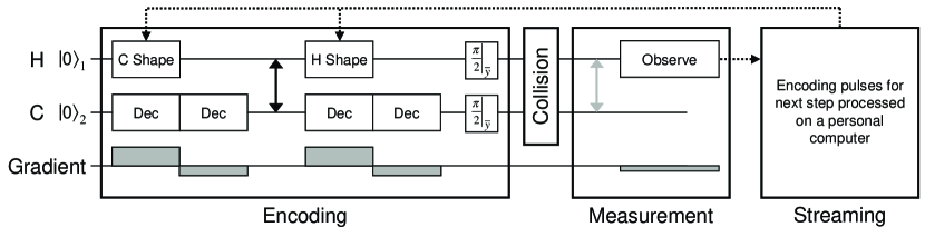
Figure 2: The NMR implementation consists of four main sections, each corresponding to the prescribed QLG algorithm step. The top two lines in the diagram correspond to RF pulses applied to the proton and carbon qubits, respectively. The third line shows the application of magnetic field gradients. In the encoding section, the initial carbon magnetization is recorded on the protons before being transferred to the carbons. The starting magnetization is specified by using a RF pulse shaped as the Fourier transform of the desired magnetization. The shaped pulses are applied in the presence of gradients so that each site can be addressed. A carbon decoupling sequence prevents the scalar coupling from interfering with the low power shaped pulses. The $\pi/2$ at the end of the encoding move the information form the x-axis to the z-axis, as required by the QLG algorithm. The collision operator follows the encoding, and it is implemented without gradients to ensure that all of the sites in the sample feel the same transformation. The results are observed in two experiments, each time using the more sensitive proton channel. A swap gate is added when measuring the carbon magnetization. Finally, the streaming operation is applied by shifting the frequencies of the carbon and proton shapes in opposite directions.

The Fourier transform approximation allows encoding of arbitrary shapes on the various spatial locations of one uncoupled nuclear species. For QIP, however, coupled spins are required to implement two-spin operations. In particular, the chloroform carbons and protons are coupled together via the scalar coupling. Given that the required RF waveforms should be weak, the coupling interferes with the desired evolution. The effect of the coupling present while encoding on spin 1 is removed by applying a strong RF decoupling sequence on the second spin decoupling . The decoupling modulates the $\sigma_{z}^{2}$ operator in the interaction Hamiltonian, making its average over a cycle period equal to zero. As a result, the second spin feels an identity operation during the decoupling. Fig. 2 shows the complete RF and gradient pulse sequence. As can be seen from the diagram, the first encoding on qubit 1 was subsequently swapped to qubit 2, followed by a re-encoding of qubit 1. We chose this method because the smaller gyromagnetic ratio of ¹³C causes a narrower frequency dispersion in the presence of the gradients, making the carbon decoupling simpler.

As described above, the encoding process writes the desired shapes in the spatial dependence of each spin’s x-magnetization. The occupation numbers, however, are proportional to the z-magnetization, as can be seen when the number operator in the equation

$$f_{a}(n,m)=\langle\psi(n,m)|{\hat{n}_{a}}|\psi(n,m)\rangle,$$ (29)

is replaced with $\hat{n}_{a}=\frac{1}{2}(1+\sigma_{z}^{a})$ resulting in

$$f_{a}(n,m)=\frac{1}{2}\left[1+\langle\psi(n,m)|{\sigma^{a}_{z}}|\psi(n,m)\rangle\right].$$ (30)

where second term in the brackets represents the z-magnetization. The encoding process is followed by a $\pi/2$ pulse that rotates the excited x-magnetization to the z direction.

IV.3 Collision and Swap Gates

After initialization, the next step is to apply the collision operator. For the QLG algorithm solution to the diffusion equation, the collision operator $\hat{C}$ is the square-root of swap gate. Expressed in terms of the Pauli operators, it is

$$\hat{C}=\text{exp}\left[-i\frac{\pi}{8}\left(\sigma^{1}_{x}\sigma^{2}_{x}+\sigma^{1}_{y}\sigma^{2}_{y}+\sigma^{1}_{z}\sigma^{2}_{z}\right)\right]$$ (31)

where an irrelevant global phase has been ignored. Written in this form, the operation $\hat{C}$ can be decomposed into a sequence of implementable RF pulses and scalar coupling evolutionsNMRQIPBasics1 ; NMRQIPBasics2 by noticing that the product operators in the exponent commute with each other, resulting in

$$\hat{C}=\text{exp}\left[-i\frac{\pi}{8}\sigma^{1}_{y}\sigma^{2}_{y}\right]\\ \text{exp}\left[-i\frac{\pi}{8}\sigma^{1}_{z}\sigma^{2}_{z}\right]\\ \text{exp}\left[-i\frac{\pi}{8}\sigma^{1}_{x}\sigma^{2}_{x}\right]$$ (32)

Expanding the first and last exponentials as scalar couplings sandwiched by the appropriate single-spin rotations results in

$$\hat{C} = \text{exp}\left[i\frac{\pi}{4}\sigma^{1}_{x}\right]\text{exp}\left[i\frac{\pi}{4}\sigma^{2}_{x}\right]\text{exp}\left[-i\frac{\pi}{8}\sigma^{1}_{z}\sigma^{2}_{z}\right]\text{exp}\left[-i\frac{\pi}{4}\sigma^{1}_{x}\right]\text{exp}\left[-i\frac{\pi}{4}\sigma^{2}_{x}\right]\cdot$$

$$\text{exp}\left[-i\frac{\pi}{8}\sigma^{1}_{z}\sigma^{2}_{z}\right]\cdot$$

$$\text{exp}\left[-i\frac{\pi}{4}\sigma^{1}_{y}\right]\text{exp}\left[-i\frac{\pi}{4}\sigma^{2}_{y}\right]\text{exp}\left[-i\frac{\pi}{8}\sigma^{1}_{z}\sigma^{2}_{z}\right]\text{exp}\left[i\frac{\pi}{4}\sigma^{1}_{y}\right]\text{exp}\left[i\frac{\pi}{4}\sigma^{2}_{y}\right]$$

The exponents of terms proportional to $\sigma^{1}_{z}\sigma^{2}_{z}$ represent internal Hamiltonian evolutions lasting for a time $t_{zz}^{col}=1/(4J)$. The exponents of terms with single-spin operators are implemented by $\pi/2$ rotations. They were generated by RF pulses whose nutation rate was about 50 times greater than $J$. All of the pulses and delays were applied without a magnetic field gradient in order to transform all of the sites identically.

As shown in Fig. 2, swap gates were utilized both in the lattice initialization and in the measurement of the carbon magnetization. The pulse sequence for the swap gates was almost identical to the sequence for $\hat{C}$. The only difference was that the internal evolution delay was set to $t_{zz}^{swap}=1/(2J)$.

IV.4 Measurement

The occupation numbers resulting from the collision were obtained by measuring the $z$-magnetizations and using equation (30). Since only the $\sigma^{a}_{x}$ and $\sigma^{a}_{y}$ operators are directly observable, a “read out” $\pi/2$ pulse transformed the $z$-magnetization into $x$-magnetization. The proton magnetization was measured directly after the collision, while the carbon magnetization was first swapped to the protons before observation. Measurements of both the ¹³C and ¹H magnetizations were carried out separately, and in both cases via the more sensitive proton channel. The measurements were made in the presence of a weak linear magnetic field gradient, causing signals from different sites to resonate with distinguishable frequencies. The observed proton signal was digitized and Fourier transformed to record an image of the spatial variation of the spin magnetization. The observed spectrum was then processed to correct the baseline and to obtain the resulting magnetization at each site. Because each site is composed of a slice of the sample with spins resonating in a band of frequencies, the occupation number for each site was obtained by averaging over all spins in the corresponding band.

IV.5 Streaming

The final step involves classically streaming the results of the measurements according to equations (14) and (15). The streaming operation is applied in conjunction with the next lattice initialization step by adding a linearly varying phase to the Fourier transform of the desired shape. The added phase causes a shift in the frequency of the pulse determined by the slope of the phase. When the frequency-shifted pulse is applied in the presence of the magnetic field gradient, the shift results in spatial translation of the encoded shape. The streaming operation is thus implemented as a signal processing step in the lattice initialization procedure.

V Results and Discussion

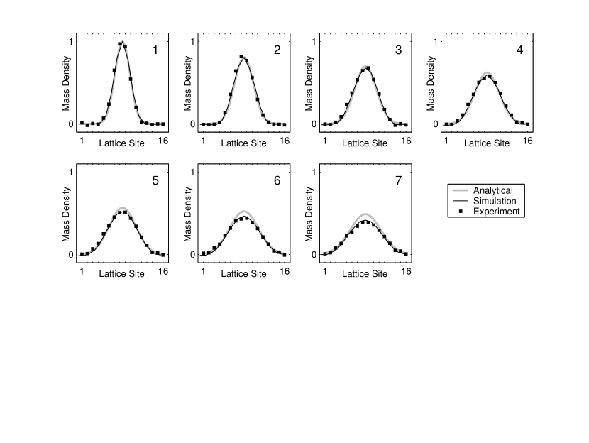
Figure 3: The experimental mass densities are plotted in the figure, together with plots of the analytical solution and the numerical simulation of the NMR experiment. The normalized, dimensionless mass densities are plotted as they were encoded on the lattice. Seven steps of the algorithm were implemented on 16 two-qubit sites. The simulations were performed using the actual RF nutation rates and times of the experimental setup. The calculations closely match the data, suggesting that the deviation between the analytical results and the data can be attributed imperfections in the methodology. As a result, the simulations promise to be useful in exploring the errors from alternate methods.

The results of the experiment are shown in Fig. 3, together with plots of the analytical solution and of numerical simulations of the NMR experiment. In total, 7 steps of the algorithm were completed using a parallel array of 16 two-qubit ensemble NMR quantum processors. The observed deviations between the data points and the analytical plots can be attributed to imperfections in the various parts of the NMR implementation.

To explore the source and relative size of these errors, we simulated perfect experiments, each time adding controlled errors in four sections of the implementation:

• Fourier transform approximation in the initialization

• Decoupling during the initialization

• Encoding swap gate and $\pi/2$ pulse errors

• Collision gate errors

The Fourier transform approximation executes a correct writing of the desired magnetization to first order in the overall flip angle. To explore errors introduced by the approximation, we simulated NMR experiments using nutation angles ranging from $\pi/2$ to $\pi/20$. In this range, angles smaller than $\pi/4$ resulted in accurate encodings of the desired Gaussian shapes through the ten steps of the implementation. The errors in the three remaining sections were simulated by using RF pulses with the actual time and nutation rate that were used on the spectrometer. By using a finite power, errors from imperfect averaging of the scalar coupling could be observed. Errors in the collision gate caused the least impact to the mass density, followed by errors originating from the imperfect decoupling sequence. The largest deviations originated from realistic simulations of the swap gate and the $\pi/2$ pulses in the encoding. It is important to note that the simulated gate fidelities for the swap and collision gates, although imperfect, are still about $0.995$. This suggests that the observed deviations are caused by the coherent buildup of errors through a few iterations, and not just by the individual errors from a single gate. The complete simulation, using realistic RF pulses and a shaped pulse nutation angle of $\pi/4$, is plotted in Fig. 3. The calculated mass densities closely match the experimental results, suggesting that the observed errors are accurately modeled.

Other potential sources of errors include the finite signal to noise, the state fidelity of the starting pseudo pure state, and gradient switching time. In addition, spin relaxation, random self-diffusion of the liquid molecules, and RF inhomogeneity can all cause attenuations in the strength of the signal. In our experiments, these last three mechanisms manifested themselves indirectly through reduced signal to noise. However, given that this attenuation was present in all of the experiments, any direct results were mostly normalized away in the data processing. Although none of the above errors contributed significantly to our implementation, they are likely to become important as more complicated algorithms are executed on larger lattices.

In particular, molecular diffusion over the time of an operation places a lower bound on the physical size of the volume element corresponding to each site in the computation. In the 1-D case discussed here, the root-mean-squared displacement ($\Delta z=\sqrt{2Dt}$) for chloroform ($D=2.35\times 10^{-5}cm^{2}/s$) is about $10.8\mu m$ over the $25ms$ needed for encoding and the collision operator. Since the actual volume element were about $625\mu m$ across, this resulted in a negligible mixing of the information in adjacent sites. However, it is clear that for this approach to type-II quantum computer to remain viable for large matries and more complex collision operators the physical size of the sample must grow with the size of the problem.

VI Conclusion

Ensemble NMR techniques have been used to study the experimental details involved in quantum information processing. The astronomical number of individual quantum systems ($\sim 10^{18}$) present in typical liquid-state spin ensembles greatly facilitates the problem of measuring spin quantum coherences. In addition, the ensemble nature has been successfully utilized to create the necessary pseudopure statesCoryPP ; IkePP and to systematically generate nonunitary operations over the ensembleHavelGradDiff . In this experiment, we again exploit the ensemble nature, but this time as a means of realizing a parallel array of quantum information processors. The novel architecture is then used to run a quantum lattice gas algorithm that solves the 1-D diffusion equation.

The closeness of the data to the analytical results is encouraging, and it demonstrates the possibility of combining the advantages of quantum computation at each node with massively parallel classical computation throughout the lattice. Currently, commercial MRI machines routinely take images with $256\times 256\times 256$ volume elements. As a result, the large size of the NMR ensemble provides, in principle, sufficient room to explore much larger lattices. However, in moving to implementations with more computational power, several challenges remain. The limited control employed here is sufficient for a few time steps of the algorithm, but refinements are necessary to increase the number of achievable iterations. In addition, although complicated operations have been done in up to 7 NMR qubitsSevenQubits1 ; SevenQubits2 ; SevenQubits3 , the problem of efficiently initializing a large lattice of few-qubit processors still remains. Our results provide a first advance in this direction, and they provide confirmation that NMR techniques can be used to test these new ideas.

VII Acknowledgments

We thank E.M. Fortunato and Y. Liu for valuable discussions. This work was supported by the Air Force Office of Scientific Research.

References

- (1) M. A. Nielsen and I. L. Chuang, Quantum Computation and Quantum Information, Cambridge University Press, Cambridge, 2000).
- (2) J. Yepez, International Journal of Modern Physics C 9 1587 (1998)
- (3) D. A. Meyer, J. Statist. Phys. 85 551 (1996)
- (4) J. Yepez, International Journal of Modern Physics C 12 1285 (2001)
- (5) D. A. Meyer, Philos T Roy Soc A 360 395 (2002)
- (6) B. M. Boghosian and W. Taylor, Phys. Rev. E 57 54 (1998)
- (7) J. Yepez, International Journal of Modern Physics C 12 1273 (2001)
- (8) J. Yepez, Quantum Computing and Quantum Communications, Lecture Notes in Computer Science, Springer-Verlag, 480 (1999)
- (9) R.R. Ernst, G. Bodenhausen, and A. Wokaun, Principles of Nuclear Magnetic Resonance in One and Two Dimensions, Oxford University Press, Oxford (1994)
- (10) D.G. Cory, M.D. Price, and T.F. Havel, Physica D 120 82 (1998)
- (11) J.A. Jones, Progress in Nuclear Magnetic Resonance Spectroscopy 38 325 (2001)
- (12) A.N. Emerton, P.V. Coveney, and B.M. Boghosian, Phys. Rev. E, 56 1286 (1997)
- (13) S. Chen, G.D. Doolen, K. Eggert, D. Grunau, and E.Y. Loh, Phys. Rev. A, 43 7053 (1991)
- (14) C. Appert and S. Zaleski, Phys. Rev. Lett., 64 1 (1990)
- (15) D.H. Rothman and S. Zaleski, Reviews of Modern Physics (1994)
- (16) R. Brito and M.H. Ernst, Physical Review A, 46:2 875 (1992)
- (17) S.P. Das, H.J. Bussemaker and M.H. Ernst, Physical Review E, 48:1 245 (1993)
- (18) B.M. Boghosian, Physical Review E, 52:1 (1995)
- (19) G.R. McNamara and G. Zanetti, Physical Review Letters, 61:20 2332 (1988)
- (20) S. Succi, R. Benzi and F. Higuera, Physica D, 47 219 (1991)
- (21) H. Chen, S. Chen and W. H. Mattaeus, Physical Review A, 45:8, R5339 (1992)
- (22) U. Frisch, B. Hasslacher and Y. Pomeau, Physical Review Letters, 56:14 1505 (1986)
- (23) J.P. Rivet and U. Frisch, Comptes Rendus, 302 267 (1986)
- (24) P. Grosfils, J. Boonm, R. Brito, and M.H. Ernst, Physical Review E, 48:4 2655 (1993)
- (25) J. Yepez, Journal of Statistical Physics 107 203 (2002)
- (26) J. Yepez, G. Vahala, L. Vahala, Submitted for publication, (2002).
- (27) I.L. Chuang, N. Gershenfeld, and M. Kubinec, Phys. Rev. Lett. 80 3408 (1998)
- (28) D.G. Cory, A.F. Fahmy, and T.F. Havel, Proceedings of the National Academy of Sciences 94 1634 (1997)
- (29) N.A. Gershenfeld and I.L. Chuang, Science 275 350 (1997)
- (30) M. Pravia, E. Fortunato, Y. Weinstein, M.D. Price, G. Teklemariam, R.J. Nelson, Y. Sharf, S. Somaroo, C.H. Tseng, T.F. Havel, and D.G. Cory, Concepts in Magnetic Resonance 11 225 (1999)
- (31) A.N. Garroway, P.K. Grannell, and P. Mansfield, Journal of Physics C 7 L457 (1974)
- (32) A. Sodickson and D.G. Cory, Progress in Magnetic Resonance 33 78 (1998)
- (33) T.F. Havel, Y. Sharf, L. Viola, and D.G. Cory Physics Letters A 280 282 (2001)
- (34) The decoupling was accomplished by applying the pulse cycle during the positive and negative gradients. The element is a composite pulse implemented with four sequential pulses having nutation angles and respective phases . This composite pulse was chosen over more commonly used pulse sequences for its relatively short total nutation angle and good decoupling, allowing the cycle to fit within a gradient period.
- (35) E. Knill, R. Laflamme, R. Martinez, and C.H. Tseng Nature 404 368 (2000)
- (36) L.M.K. Vandersypen, M. Steffen, G. Breyta, C.S. Yannoni, R. Cleve, and I.L. Chuang Phys. Rev. Lett. 85 5452 (2000)
- (37) L.M.K. Vandersypen, M. Steffen, G. Breyta, C.S. Yannoni, M.H. Sherwood, and I.L. Chuang Nature 414 883 (2001)