Hamiltonian monodromy as lattice defect

Abstract

The analogy between monodromy in dynamical (Hamiltonian) systems and defect in crystal lattices is used in order to formulate some general conjectures about possible types of qualitative features of quantum systems which can be interpreted as a manifestation of classical monodromy in quantum finite particle (molecular) problems.

1 Introduction

The purpose of this paper is to demonstrate amazing similarity between apparently different subjects: defects of regular periodic lattices, monodromy of classical Hamiltonian integrable dynamical systems, and qualitative features of joint quantum spectra of several commuting observables for quantum finite-particle systems. First of all we recall why regular lattices and lattices with defects appear naturally for classical integrable Hamiltonian systems and for their quantum analogs. Then we describe several “elementary dynamical” defects using tools and language developed in the theory of crystal defects. Comparison between defects arising in dynamical systems and crystal defects leads to many interesting questions about possibility of realization of certain defects in Hamiltonian dynamics and in crystals.

2 Integrable classical singular fibrations and monodromy

Let us start with the example of Liouville integrable classical Hamiltonian system with $N$ degrees of freedom Arnold . This means that there exists a set $F=\{F_{1},\ldots,F_{n}\}$ of functions defined on $2n$-dimensional symplectic manifold $M$, which are functionally independent and mutually in involution. The Hamiltonian $H$ can be locally represented as a function $H=f(F_{1},\ldots,F_{n})$. The mapping $F:M\rightarrow R^{n}$ defines the integrable fibration. We call it a generalized energy-momentum map. Each fiber is the union of connected component of inverse images $F^{-1}(f)$ of points $f\in R^{n}$. If the differentials $\{dF_{1},\ldots,dF_{n}\}$ of functions from $F$ are linearly independent in each point the fibration is called regular. If moreover all fibers are compact, the fibration is toric. We will be interested in integrable toric fibrations with singularities of some simplest type.

Let us restrict ourselves to systems with two degrees of freedom. Typical examples of images of singular energy-momentum maps are shown in Figure 1. The isolated critical value of the map $F$ (see Figure 1, left), also known as focus-focus singularity Lerman ; zung97 , appears, for example, for such problems as spherical pendulum cushman83 ; Duist80 ; cushman-duistermaat88 , champagne bottle Bates ; cushman-bates , coupling of two angular momenta SadZhPhysLett , etc. The singular fiber in this case is a pinched torus (Figure 2, left) with one isolated critical point of rank 0.

Presence of a half-line of critical values, together with end point, is typical for nonlinear $1:(-k)$ resonant oscillator NekhSadZhil . Each point on the singular half-line corresponds to singular “curled torus” (Figure 2, center shows curled torus for the case $k=2$) NekhSadZhil ; ColinSan , which differs from an ordinary torus due to presence of one circular trajectory which covers itself $k$-times. This particular circular trajectory is formed by critical points of rank 1 of the map $F$. The end point (see Figure 1, center) corresponds to pinched curled torus with multiple circle shrinking to a point. This fiber has one critical point of rank 0 and is topologically equivalent to pinched torus but its immersion into $4D$-space is different. A pinched curled torus for $k=2$ is shown in Figure 2, right.

           

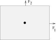
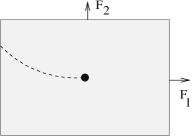
Figure 1: Examples of images of the energy momentum maps for singular toric fibrations.

           

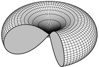
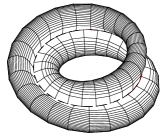
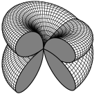
Figure 2: Singular fibers. Pinched torus (left). Curled torus (center). Pinched curled torus (right).

More general situation with two singular rays starting at one singular point (as shown in Figure 2, right) corresponds to $k:(-l)$ resonant nonlinear oscillator. Example of the integrable fibration corresponding to all shown in Figure 1 images of the energy-momentum maps with two integrals $(F_{1},F_{2})$ in involution can be written as NekhSadZhil

$$F_{1} = m_{1}{\textstyle\frac{1}{2}}(p_{1}^{2}+q_{1}^{2})-m_{2}{\textstyle\frac{1}{2}}(p_{2}^{2}+q_{2}^{2}),$$ (1)

$$F_{2} = {\rm Im}\bigl{[}(q_{1}+ip_{1})^{m_{2}}(q_{2}+ip_{2})^{m_{1}}\bigr{]}+\bigl{(}m_{1}{\textstyle\frac{1}{2}}(p_{1}^{2}+q_{1}^{2})+m_{2}{\textstyle\frac{1}{2}}(p_{2}^{2}+q_{2}^{2})\bigr{)}^{s},$$ (2)

with $s>(m_{1}+m_{2})/2$, and $m_{1},m_{2}$ positive integers.

All regular fibers are two-dimensional tori. Their fundamental groups are abelian groups $Z^{2}$ with two generators, corresponding to two basic cycles on a torus. The fundamental groups for different regular tori are isomorphic among themselves and to $Z^{2}$ integer lattice. We can establish the correspondence between basic cycles defined on different tori by choosing a continuous path in the $4D$-space which is transversal to fibers and by deforming basic cycles continuously along this path. In particular, for a closed path passing only through regular tori we get the automorphism of the fundamental group of a chosen regular torus. The corresponding map of basic cycles is the monodromy map. It is the same for all homotopy equivalent closed paths. If the path crosses singular lines similar to those taking place for integrable fibration of the (1,2) resonance oscillators only subgroup of chains can be continuously deformed along the path and the monodromy map in such a case can be defined only for a subgroup of fundamental group NekhSadZhilinpress . Nevertheless this map can be linearly extended to a whole group. In this case the extended monodromy map is represented by a matrix with fractional entries; while in the case of isolated critical values the monodromy map is given by integer matrix $\mu\in SL(2,Z)$.

3 Quantum monodromy

In order to study the manifestation of classical monodromy in associated quantum problems we first need to recall the existence of local action-angle variables Arnold ; NNaav and to replace the transformation of angles by corresponding transformation of actions. In the case of locally regular integrable fibrations local action-angle variables $\{I_{k},\phi_{k}\}$ exist and the linear transformation of angles $\phi^{\prime}=M\phi$, imposed by the monodromy map, corresponds to the transformation of actions $I^{\prime}=\left(M^{-1}\right)^{\dagger}I$.

For quantum problems we are interested in the joint spectrum of commuting operators, corresponding to classical integrals $\{F_{1},F_{2}\}$ grondin-sadovskii-zhilinskii ; Vu1 ; waalkens-dullin ; child-weston-tennyson . The collection of joint eigenvalues superimposed on the image of the energy-momentum map for classical problem reveals locally the presence of a regular lattice associated with integrality conditions imposed on local actions by quantum mechanics. The lattice of quantum states for quantum problem corresponding to classical oscillators with $1:(-1)$ and $1:(-2)$ resonances is represented in Fig. 3 NekhSadZhil .

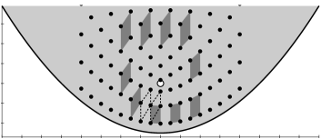
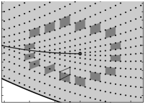
Figure 3: Example of the lattice of quantum states with monodromy. Resonant oscillators (1,2) with $m_{1}=m_{2}=1$ (left) and $m_{1}=1$, $m_{2}=2$ (right).

Due to existence of monodromy, lattice of quantum states can not be regular globally. From figure 3 it is clearly seen that the transport of elementary cell of the locally regular part of the lattice around the singularity shows nontrivial monodromy for a non-contractible close path in the base space (in the space of $F_{1},F_{2}$ values). The presence of quantum monodromy can be interpreted as a presence of defects of locally regular lattice of quantum states SadZhPhysLett . In the case of isolated critical values of classical problem (Figure 3, left) the choice of elementary cell is arbitrary and the monodromy map is integer. In the case of the presence of singular line at the image of the classical energy momentum map, the dimension of the cell should be increased (doubled in the case of $1:(-2)$ resonance) in order to ensure the unambiguous crossing of the singular line NekhSadZhil . In both cases the presence of singular fibers in classical problem is reflected in the appearance of some specific defects of the lattice of quantum states for corresponding quantum problem. We want now to describe these specific defects arising in the quantum theory of Hamiltonian systems using methods and tools from defect theory of periodic lattices Kleman ; Mermin ; Michel ; Kroner .

4 Elementary defects of lattices

Let us play with analogy between 2-D lattice of quantum numbers (or of action variables in the classical limit) and the 2-D lattice of regular solid with defects. More precisely the idea is to see the correspondence between defects of periodic solids and monodromy which is an obstruction to the existence of global action-angle variables in Hamiltonian dynamics (for integrable systems).

For 2-D system each quantum state (or a site for a lattice formed by points) is characterized by two numbers, say $(n_{1},n_{2})$. The existence of local order means that starting with some vertex (point of the lattice) one can form two vectors, or equivalently the elementary cell of the lattice by defining two vectors as joining respectively $(n_{1},n_{2})$ with $(n_{1}+1,n_{2})$ and with $(n_{1},n_{2}+1)$. This corresponds to the choice of the elementary cell with four vertices $\{(n_{1},n_{2}),(n_{1}+1,n_{2}),(n_{1},n_{2}+1),(n_{1},n_{2}+1)\}$. The choice of the elementary cell (or equivalently the choice of the basis of the lattice) is not unique. It is defined only up to arbitrary transformation with matrix $M\in SL(2,Z)$. But let us fix some choice for a moment. The existence of local actions in quantum-state lattice language means that by elementary translations in two directions we can label unambiguously all vertices by two numbers with difference in numbers along each edge being 1 for one number and 0 for another. This means that there is no defects (in the local region studied).

Let us now analyze several different types of defects which can be imagined for periodic lattices in order to find possible candidates to represent defects of lattices of quantum numbers for quantum problems corresponding to classical Hamiltonian systems with non-trivial (integer and fractional) monodromy.

4.1 Vacations and linear dislocations

The simplest point defect well known in solids is the absence of vertex (or the presence of additional vertex). This defect does not distort the system of edges not connected with the vacation. The lattice is not deformed even slightly away from the point defect. The elementary cell after a circular trip around the vacation has no modifications. See Fig. 4, left.

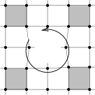
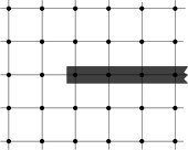
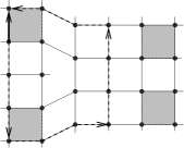
Figure 4: Lattice with vacation (left). Construction of linear dislocation (centre). Lattice with linear dislocation (right).

Linear dislocation can be easily imagined to be formed through the following formal procedure. Let us remove all vertices on the half-line started at a given vertex and join the vertices though the gap (see Fig. 4, center). Equally, after making a cut along a line of vertices we can introduce additional (one or even several) half-lines. Now the circular path around this defect will show us the existence of the defect. To observe this defect we should go around it by doing the same number of steps in four directions (say, down, right, up, and left). If the final point will not be the same as the initial point, there is a defect. The vector from initial point to the final point (Burgers vector in solid state physics) characterizes the dislocation. Observe that the elementary cell after the round trip around the dislocation will return exactly to its initial place (see Fig. 4, right) because Burgers vector does not depend on the initial point and it is exactly the same for all four vertices of the cell. This means that vacation and linear dislocations can not be associated with monodromy type defects of regular lattices.

4.2 Angular dislocations as elementary monodromy defect

Another general idea to form defect starting from the regular lattice is to remove or to introduce “the solid angle” and to establish in some way the regular correspondence between two boundaries everywhere except one central point.

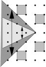
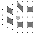
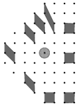
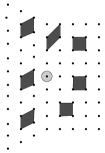
Figure 5: Construction of the angular dislocation by removing or adding one of the solid angles shown on the left picture. Reconstructed lattices after removing or adding small or large sectors are shown together with transport of elementary cell along a closed path around the defect on the reconstructed lattice. The identification of boundaries after removing or adding solid angle is done by the parallel shift of lattice points in vertical direction.

It is important to note that correspondence between two boundaries should be imposed in order to reconstruct the lattice. We will look for different possibilities but let us start with the simplest one: After removing (or introducing) the solid angle, the reconstruction is d.ne by the parallel shift of lattice points in one chosen direction. The requirement for reconstructed lattice to be well defined everywhere except singular point can be satisfied only for some special values of removed or added angles. Namely we should impose that the number of removed (added) points at each vertical line is integer and varies linearly with distance from the vertex of the solid angle. Figure 5, left shows examples of removed or added solid angles. Two different solid angles correspond respectively to removing (adding) of one or two additional points from vertical line at each step in the horizontal direction. We can remove or add solid angles in different ways. Figure 6 illustrates the construction of the removed angle. We start with one chosen point $O$ of the lattice and two basis vectors corresponding to “horizontal” and “vertical” directions. We put the first cut through the vertex $A$ lying at the $k$-th vertical line counting from the vertex $O$. ($k=6$ on figure 6). To construct the second cut we go from $A$ in vertical direction up to $k$-th horizontal line. Two rays $OA$ and $OB$ show the sector to be removed. Observe that with this construction $s$ points are removed from $s$-th vertical line.

Figures 5 show graphically what happens with lattice after removing (or adding) solid angles. It is important to note that just by looking on the deformation of elementary cell after the round trip on the reconstructed lattice we can easily find how big was removed (added) solid angle and what transformation (removing or adding) was exactly done. The absolute value of removed (added) solid angle can be read directly by comparing the form of the initial and final cell. It is sufficient to write the transformation of two vectors forming elementary cell in matrix form. This matrix is nothing else but the monodromy matrix for actions. For two examples shown in Figure 5 this monodromy matrix has the form $\left(\begin{array}[]{cc}1&p\\ 0&1\end{array}\right)$ or $\left(\begin{array}[]{cc}1&0\\ p&1\end{array}\right)$ with $p=\pm 1$ or $p=\pm 2$. One or another form of matrix and the sign of $p$ depends on the choice of the first and second basis vector and on the direction of the circular trip (clockwise or counterclockwise). At the same time the absolute value of $|p|$ is unambiguously related with the absolute value of the removed (added) solid angle.

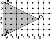
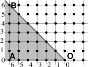
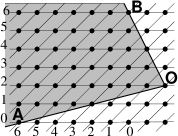
Figure 6: Alternative constructions of the same defect.

More subtle arguments are needed to distinguish between adding and removing solid angle with the same $|p|$. We will denote below defects obtained by removing solid angle by $(-)$ and by adding solid angle by $(+)$.

4.3 About the sign of the elementary monodromy defect

The existence of the sign of Hamiltonian monodromy was conjectured by the author on the basis of analogy between monodromy and $(+)$ and $(-)$ defects of lattices. The proof was given by Cushman and Vu Ngoc CushmanSan . We give here the characterization of the sign of defect in terms of lattice transformation.

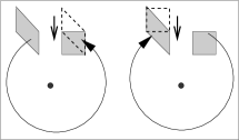
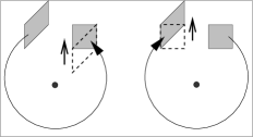
Figure 7: Comparison of initial and final cells after the circular path around the singularity on the lattice reconstructed after removing [$(-)$ defect, left] or adding [$(+)$ defect, right] elementary solid angle. Both counterclockwise and clockwise circular paths are shown for each type of defects.

Let first compare initial and final cells for the same reconstructed lattice (with $|p|=1$) obtained by removing simplest solid angle but for both kinds of circular paths (clockwise and counterclockwise). See Fig. 7, left. The identification of initial cell with the final one can be done only for two vertices. We choose the identified pair being the back side of the cell in the final position (with respect to the direction given by the sense of rotation). It is clearly seen from the figure 7, left that in order to deform the initial cell for $(-)$ defect to the form of the final cell we need to move the front side of the cell in the direction inside the surrounded singularity. This result is unchanged if we apply the same procedure to the clockwise or counterclockwise circular path.

A similar analysis can be done for lattice reconstructed after adding solid angle, i.e. for $(+)$ defect, (see Fig. 7, right) shows that the deformation of the initial cell after the round trip is now in the outside direction with respect to the surrounded singularity. This result remains again the same for both clockwise and counterclockwise direction of the circular path.

Thus the simple geometrical analysis of the transformation of elementary cell enables one to associate with elementary monodromy the specific defect of the regular lattice. The defect obtained by removing solid angle with $|p|=1$ will be called the elementary monodromy defect. Exactly this defect appears in lattices of quantum states for Hamiltonian systems corresponding to classical Hamiltonian systems with focus-focus singularities. Observe that defects with $|p|>1$ appear naturally in Hamiltonian systems with symmetries. One of the most interesting and physically important systems of this kind is the integrable approximation for hydrogen atom in crossed electric and magnetic fields cushman-sadovskii00 . In classical systems monodromy with $|p|>1$ corresponds to presence of isolated singular fiber which is $|p|$-times pinched torus matveev . Cushman and Vu Ngoc CushmanSan have proved that only focus-focus singularities with the same sign of monodromy can appear in a connected component of of the image of the generalised energy momentum map of an integrable Hamiltonian system. In non-Hamiltonian systems monodromy of both sign can appear simultaneously cushman-duistermaatNH .

4.4 Rational cuts and rational line defects

We have seen in previous section that only very special cuts together with matching rules enables us to construct the point defects. Now we will generalize the admissible cuts but keep the matching rule. Let us start with the example of $1:2$ rational cut which is defined as follows (see Figure 8).

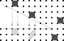
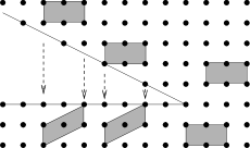
Figure 8: Construction of the $1:2$ rational lattice defect starting from the regular square lattice. (Left) - Ambiguity in the transfer of $1\times 1$ cell through the cut. (Right) - Unambiguous transfer of double cell through the cut.

We cut out half of the solid angle removed in the case of the elementary monodromy defect. After removing this solid angle the two boundaries are different. At one (lower boundary on Figure 8) points are situated at each vertical line of the lattice. At the upper boundary of the cut points are situated only at each second vertical line. We keep the matching rules, i.e. identify the boundaries by sliding points along the vertical lines. Naturally, the reconstructed lattice is not homogeneous along the identified boundary. It is seen from the fact that the number of removed points from vertical lines varies like $0,0,1,1,2,2,3,3,\ldots$ along the horizontal direction. (Remark. The number of removed points can be represented in the form of the sum of linear and oscillatory functions.) This means that the reconstructed lattice has a line defect.

If we try to pass the elementary cell of the lattice through the cut the result depends on the place where the cell goes through the boundary line. From Figure 8, left, it is clear that when the right side of the cell goes through the cut at even vertical line (supposing the vertical line going through the vertex of the removed sector to be even) the form of the elementary cell remains unchanged. In contrast, when the right side of the cell goes through the cut at odd vertical line, the form of the cell changes. This ambiguity can be avoided if instead of elementary $1\times 1$ cell we will use larger cell. Namely, we double the dimension of the cell in the horizontal direction. The double cell passes through the cut at any place in a similar way. But the internal structure of the cell changes after crossing the line defect. Cell transforms from “face centered” to “body centered” in the crystallographic terminology. But this modification is uniform along the cut. In some way, by increasing the dimension of the cell we neglect the effects comparable with the dimension of the cell. This enables us to define the transformation of lattice vectors after traversing a closed path around the origin of the removed sector. Putting $e_{h}$ and $e_{v}$ as horizontal and vertical basis vectors of the square lattice shown in Figure 8 and $\{e_{v},e_{h}^{double}=2e_{h}\}$ as vectors forming the double cell, the transformation of vectors forming the double cell after a close path around the origin of the removed sector in the counterclockwise direction is

$$\left(\begin{array}[]{c}e_{v}^{\prime}\\ (e_{h}^{double})^{\prime}\end{array}\right)=\left(\begin{array}[]{cc}1&\ 0\\ 1&\ 1\end{array}\right)\left(\begin{array}[]{c}e_{v}\\ e_{h}^{double}\end{array}\right).$$ (3)

If we extend linearly this transformation to lattice vectors themselves the transformation matrix takes the form

$$\left(\begin{array}[]{c}e_{v}^{\prime}\\ e_{h}^{\prime}\end{array}\right)=\left(\begin{array}[]{cc}1&\ 0\\ 1/2&\ 1\end{array}\right)\left(\begin{array}[]{c}e_{v}\\ e_{h}\end{array}\right).$$ (4)

The so obtained matrix with fractional entry coincides with the fractional monodromy matrix for actions in the case of $1:(-2)$ resonant classical oscillator and with quantum fractional monodromy for corresponding quantum problem.

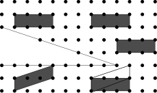
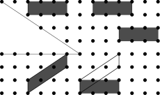
Figure 9: Construction of the $1:3$ and $2:3$ rational lattice defects starting from the regular square lattice.

Using the same principle we can construct, for example, line defects by reconstructing lattice after $1:3$ or $2:3$ rational cuts shown in Figure 9. This notation means that we remove the solid angle $\varphi=\tan^{-1}(1/3)$ or $\tan^{-1}(2/3)$ respectively. We need to triple the dimension of cell in the horizontal direction in order to get unambiguous transformation rules for the cell after crossing the line defect on the reconstructed lattice. It is clear from the Figure 9 that the monodromy matrices for $1:3$ and $2:3$ rational defects have respectively the form $\left(\begin{array}[]{cc}1&0\\ 1/3&1\end{array}\right)$ and $\left(\begin{array}[]{cc}1&0\\ 2/3&1\end{array}\right)$. Removing $2:3$ rational solid angle is equivalent to removing twice the $1:3$ rational solid angle. Generalization to arbitrary rational cut with the same type of matching rules for reconstruction of the lattice is quite obvious and leads to half-line defect with fractional monodromy matrix.

We can also suggest alternative matching rules after rational cuts with the idea to obtain reconstructed lattice with only point rather than the line defect. Let us consider again as example the $1:3$ rational cut but with different matching rules for two boundaries (see Figure 10).

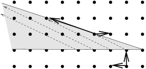
Figure 10: Matching rules for reconstruction of lattice after rational cut. Example of $1:3$ cut. The monodromy of the resulting defect is the Arnol’d cat map.

It is clear that if we want to have on the reconstructed lattice only point defect all vertices on two boundaries should be consecutively identified. This identification imposes matching rule for one of the basis vectors of the lattice. Another should be chosen in such a way that two new basis vectors form elementary cell of the same volume, i.e. they should be related one to another with $SL(2,Z)$ transformation. In fact this matrix is precisely the monodromy matrix of the point defect just by the construction. In the case of $1:3$ rational cut shown in Fig. 10 the resulting monodromy matrix has the form $\left(\begin{array}[]{cc}0&-1\\ 1&\ \ 3\end{array}\right)$. This matrix is known as Arnol’d cat map ArnAv . A lot of different examples of point defects can be constructed in a similar way. But we will take as elementary point defect only $(-)$ defects corresponding to elementary monodromy matrix. We will demonstrate now that all other defects can be considered as more complicated objects composed in some way from several elementary ones.

5 Defects with arbitrary monodromy

We now turn to the description of defects which can be characterized by arbitrary monodromy matrices. As soon as the choice of the basis of the lattice is ambiguous, the matrix representation of the monodromy transformation is basis dependent. For example the monodromy matrix $M_{a}=\left(\begin{array}[]{cc}1&1\\ 0&1\end{array}\right)$ after the transformation to another basis through the similarity $M_{a}^{\prime}=AM_{a}A^{-1}$ with $A$ being arbitrary $SL(2,Z)$ matrix takes the form

$$\left(\begin{array}[]{cc}a&b\\ c&d\end{array}\right)\left(\begin{array}[]{cc}1&1\\ 0&1\end{array}\right)\left(\begin{array}[]{cc}d&-b\\ -c&a\end{array}\right)=\left(\begin{array}[]{cc}1-ac&a^{2}\\ -c^{2}&1+ac\end{array}\right)$$

From this family of equivalent matrices it is immediately clear that matrices $\left(\begin{array}[]{cc}1&1\\ 0&1\end{array}\right)$ and $\left(\begin{array}[]{cc}1&0\\ -1&1\end{array}\right)$ are equivalent but they are written in different frames. In contrast, matrix $\left(\begin{array}[]{cc}1&-1\\ 0&1\end{array}\right)$ is equivalent to $\left(\begin{array}[]{cc}1&0\\ 1&1\end{array}\right)$ but is not equivalent to $\left(\begin{array}[]{cc}1&1\\ 0&1\end{array}\right)$ in spite of the fact that these two matrices are mutually inversed.

In order to formulate precise statement about equivalence or in-equivalence of different defects we should first establish equivalence of $SL(2,Z)$ matrices with respect to conjugation by elements of $SL(2,Z)$, i.e. to describe classes of conjugated elements of $SL(2,Z)$ group.

It is well known that the trace and the determinant of the matrix are invariant with respect to similarity transformation. But these invariants are not sufficient to completely characterize classes of conjugated elements. Before looking for $SL(2,Z)$ matrices let us start with $SL(2,R)$ ones.

5.1 Topological description of unimodular matrices

Let consider the subspace of $SL(2,R)$ matrices $M=\left(\begin{array}[]{cc}\alpha&\beta\\ \gamma&\delta\end{array}\right)$ with ${\rm Tr}\ M=K$. This means that four matrix elements $\alpha,\beta,\gamma,\delta$ are related by two equations

$$\alpha\delta-\beta\gamma=1,\ \ \ \ \alpha+\delta=K.$$ (5)

Eliminating one parameter (say $\alpha$) we get the following relation between three parameters $\beta,\gamma,\delta$

$$-1+K\delta-\delta^{2}-\gamma\beta=0.$$ (6)

We can interpret this relation as the geometrical description of all $SL(2,R)$ matrices with given trace in the three dimensional space of parameters $\beta,\gamma,\delta$. The geometrical form of so obtained surface depends on the value of $K$. Topologically there are three different situations.

If $K=\pm 2$ we have double cone with vertex corresponding to $\pm\left(\begin{array}[]{cc}1&0\\ 0&1\end{array}\right)$ matrix. If $|K|>2$ we have a hyperboloid of one-sheet and if $-2<K<2$ we have two-sheeted hyperboloid. We can schematically represent the whole family of $SL(2,R)$ matrices by filling the solid torus in three-dimensional space of parameters by surfaces corresponding to all possible values of traces. This representation is given in Figure 11.

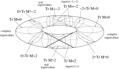
Figure 11: The topological structure of the space of 2 by 2 matrices with determinant 1. The solid tore in 3-D space is foliated by levels corresponding to a given value of the trace of matrix $M$.

The existence of two disjoint connected components for matrices with $-2\leq{\rm Tr}M\leq 2$ implies the existence of additional invariant which classifies matrices with the same trace into smaller subclasses of conjugate elements. We need such description but only for matrices in $SL(2,Z)$. The important difference between $SL(2,R)$ and $SL(2,Z)$ cases is due to the fact that there is only finite number of possible values of the trace in $SL(2,Z)$ which correspond to matrices with complex eigenvalues in $SL(2,R)$. In physical language this is the consequence of the fact that only axes of second, third, fourth and sixth orders are compatible with the existence of the lattice.

Formal proof: Characteristic polynomial for the $SL(2,Z)$ matrix $M$ has the form $\lambda^{2}-({\rm Tr}\ M)\lambda+1=0$. It has complex eigenvalues only if the discriminant $({\rm Tr}\ M)^{2}-4<0$. As soon as the trace is integer, it is only possible that $({\rm Tr}\ M)=0,\pm 1$.

Now we can return to the study of $SL(2,Z)$ case.

5.2 Classes of conjugated elements and ”normal form” of $SL(2,Z)$ matrices

The matrices $M\in SL(2,Z)$ will be named parabolic, elliptic, or hyperbolic, depending on their trace. Parabolic matrices have trace equal $\pm 2$ and their eigenvalues are $\{+1,+1\}$ or $\{-1,-1\}$. Elliptic matrices have trace $\pm 1$ or $0$. Their eigenvalues are complex numbers. Hyperbolic matrices have $|{\rm Tr}\ M|>2$. Their eigenvalues are real irrational numbers. Identity matrix $\left(\begin{array}[]{cc}1&0\\ 0&1\end{array}\right)$ and minus identity $\left(\begin{array}[]{cc}-1&0\\ 0&-1\end{array}\right)$ commute with all elements from $SL(2,Z)$ and each form a proper class of conjugate elements consisting of one element. We will consider these classes separately. In Fig, 11 these matrices correspond to vertices of double cones of matrices with trace $\pm 2$.

Within each class of conjugate elements we can choose one matrix to be the “normal form”. All classes of conjugate elements together with normal forms are listed in Table 1.

Table 1: Classes of conjugated elements of $SL(2,Z)$ group together with normal forms of matrices for each class.

Trace	$K,(|K|>2)$	$\pm 2$	$\pm 1$	$0$
Module	$-$	$p=0,\pm 1,\ldots$	$\varepsilon=\pm 1$	$\varepsilon=\pm 1$
Normal form	$\left(\begin{array}[]{cc}K&1\\ -1&0\end{array}\right)$	$\left(\begin{array}[]{cc}1&p\\ 0&1\end{array}\right)$	$\left(\begin{array}[]{cc}\pm(1+\varepsilon)/2&\varepsilon\\ -\varepsilon&\pm(1-\varepsilon)/2\end{array}\right)$	$\left(\begin{array}[]{cc}0&\varepsilon\\ -\varepsilon&0\end{array}\right)$

5.3 Several elementary monodromy defects

We have defined the construction of elementary defects using one chosen lattice basis. Both cuts and matching rules were precisely defined in that basis. But the choice of the lattice basis is not unique. If there are two defects, characterized both by elementary monodromy matrix but the choice of basis and the orientation of cuts for these two defects are different, the global monodromy, corresponding to transformation of elementary cell after a circular path around both defects, depends on relative orientation of two removed solid angles. Let us again start with some particular examples of systems with several elementary defects.

Disclinations as a composition of elementary monodromy defects

Figure 12 shows regular square lattice with three defects corresponding to elementary monodromy. For two removed angles (sectors around horizontal lines) the reconstruction of lattice is done through sliding points in vertical directions. For the third removed angle the identification of boundaries is done through the horizontal sliding of lattice points.

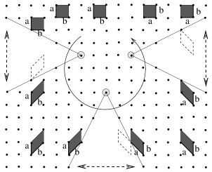
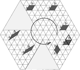
Figure 12: (Left) - Regular square lattice with three elementary monodromy defects. (Right) - Regular triangular lattice with two elementary monodromy defects.

The cumulative effect of three elementary cuts is the rotation of the elementary cell by $\pi/2$. The direction of the rotation of the elementary cell is defined by the direction of the circular path around singularities. Such defect is known in solid state physics as $\pi/2$ rotational disclination. It is easy to see that the same effect takes place if the three cuts are distributed in another way between vertical and horizontal directions (two vertical and one horizontal). To see this it is just sufficient to look at the same figure after rotating it by $\pi/2$.

Naturally, similar construction can be done with three singular points corresponding to adding the solid angle and reconnecting new boundaries through horizontal or vertical shift. The resulting effect on the elementary cell is again the $\pi/2$ rotation, but now the rotation of the elementary cell is in opposite direction (as compared to the direction of the circular loop around the singularity).

The global effect in both cases can be reproduced by removing (or adding) the solid angle $\pi/2$ and by reconstructing lattice through identification of two boundaries by rotating them as it is shown in Figure 13 where $\pi/2$ solid angle is removed. Naturally one can also remove $\pi$ or $3\pi/2$ solid angle or to add $\pi/2$ or $k\pi/2$ solid angle as it is shown in Figure 15. This gives negative or positive rotational disclinations.

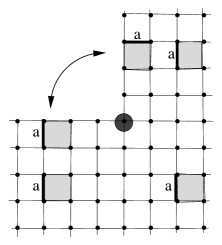
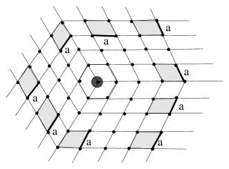
Figure 13: Construction of the rotational disclination by removing solid angle $\pi/2$ shown on the left picture.

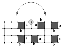
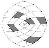
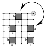
Figure 14: Construction of the rotational disclination by removing solid angle $\pi$ (Left) and $3\pi/2$ (Right). The reconstructed lattice after removing $\pi$ solid angle (center).

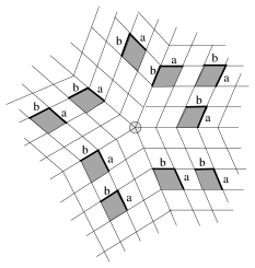
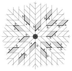
Figure 15: Construction of the rotational dislocation (disclination) by introducing solid angle $k\pi/2$. $k=1$ on the left and $k=4$ on the right picture.

The same construction made with triangular lattice and with two elementary monodromy defects rotated one with respect to another over $2\pi/3$ gives the cumulative effect consisting in rotation of elementary cell over $2\pi/6$ after a close path surrounding two elementary defects (see figure 12, right). The cumulative effects of such two elementary monodromy defects is the $\pi/3$ rotational disclination. Its multiple, positive or negative analogs can be immediately constructed.

Rotational disclinations are well known defects in the solid state physics. From the point of view of defects of quantum state lattices and classical Hamiltonian monodromy, the elementary monodromy defects seems to be more fundamental. Any rotational disclination can be constructed as a global effect in systems with several elementary monodromy defects.

Multiple defects with trivial global monodromy

Let us now consider in more general way the correspondence between local and global monodromy for a system of elementary defects. Figure 16 illustrates this relation.

Suppose we have two defects $c_{1}$ and $c_{2}$ characterized by monodromy matrices $M_{1}$ and $M_{2}$. These monodromy matrices are obtained by going around the defect $c_{i}$ starting from point $b_{i}$ and using local basis associated with point $b_{i}$. If we are interested now in global monodromy which corresponds to a close loop going around two defects and starting at initial point $b_{0}$ with its own local basis we can calculate the global monodromy by going first from $b_{0}$ to $b_{1}$, making close loop around $c_{1}$, returning back by the same way, and repeating the same for the second defect. The global monodromy calculated in this way should be the same by homotopy arguments. If the modification of the basis between $b_{0}$ and $b_{i}$ is described by matrices $A_{i}$ the global monodromy $M$ can be expressed in terms of $M_{1}$ and $M_{2}$ as $M=A_{1}M_{1}A_{1}^{-1}A_{2}M_{2}A_{2}^{-1}$.

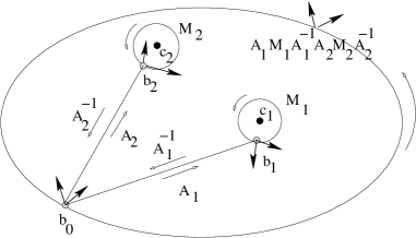
Figure 16: Relation between local monodromy matrices for isolated defects and global monodromy for the circular path around two defects

Naturally for an arbitrary system of elementary defects the global monodromy matrix can always be represented in the form $M=\prod_{i}A_{i}M_{i}A_{i}^{-1}$. As it was already noted the monodromy matrix is defined up to conjugation with $SL(2,Z)$ matrices, i.e. defects with different monodromy are in one to one correspondence with classes of conjugate elements of $SL(2,Z)$ matrices.

One can easily verify that arbitrary $SL(2,Z)$ matrix can be represented in the form of product of matrices, conjugate to elementary monodromy matrices with one chosen sign CushZhil . In particular, the identity matrix can also be represented in the form of product of matrices conjugate to elementary monodromy matrix. It is obvious that four $\pi/2$ rotational disclinations (or six $\pi/6$ rotational disclinations) give trivial global monodromy. In fact the elementary cell make a $2\pi$ rotation when going along close path surrounding these defects and in spite of the fact that the monodromy is trivial the close path is not contractible and the defect exists. An easy consequence of this statement: The monodromy matrix (defined up to conjugation with $SL(2,Z)$ matrices) is not sufficient to distinguish defects. Two defects with the same monodromy matrix can be further labeled by the number $k$ of $2\pi$ rotations of the elementary cell after a close path around a defect. This additional number $k$ can be arbitrary integer $k=0,\pm 1,\pm 2,\ldots$. Note that an elemenraty $(-)$ monodromy defect can be constructed as a cumulative effect of eleven elementary $(+)$ monodromy defects CushZhil .

One can easily obtain trivial global monodromy for a close path around two defects with different signs. Figure 17 shows construction of two elementary monodromy defects with different signs. Signs plus and minus indicate respectively adding and removing of the same solid angle.

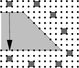
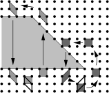
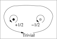
Figure 17: Lattice with two elementary monodromy defects of different sign.

5.4 Several rational line defects

Let us now discuss examples of lattices with multiple rational line defects. We assume below that all defects are of the same sign, i.e. obtained by removing solid angle. We start with example of two defects $1:2$ and $1:3$ which have similar orientation (see Figure 18, left). These two defects model the singularities of integrable toric fibration for $2:-3$ resonant oscillator (1). Elementary $1\times 1$ cell can not cross unambiguously both defect half-lines. The cell should be doubled in horizontal direction in order to cross unambiguously the $1:2$ defect. In a similar way the cell should be tripled in the same direction in order to cross the $1:3$ defect. This means that only $1\times 6$ cell which is six times larger in the horizontal direction can cross both defects. Using such cell we can go along a close path surrounding the singular vertex. After linear extension to elementary lattice vectors we get the fractional monodromy matrix $\left(\begin{array}[]{cc}1&\ 0\\ 5/6&\ 1\end{array}\right)$.

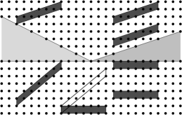
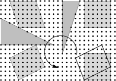
Figure 18: Construction of lattice with two rational defects, $1:2$ and $1:3$ (Left)- Parallel defects which correspond to singular one-dimensional strata for $2:(-3)$ resonance oscillator. (Right) - Two orthogonal defects.

If two rational defects, $1:2$ and $1:3$, have different orientations the situation becomes quite different. Figure 18, right shows these two defects with orthogonal orientation. In order to pass through horizontal $1:2$ defect the cell should be doubled in horizontal direction. In order to pass through $1:3$ vertical defect the cell should be tripled in vertical direction. Moreover, one should note that all vertices of the cell should lie on even vertical lines and on horizontal lines having the same number modulo 3. This means that we need to take at least $6\times 6$ cell in order to cross unambiguously both rational cuts. The resulting monodromy matrix for a counterclockwise path around two singular points has the form $\left(\begin{array}[]{cc}5/6&\ -1/3\\ 1/2&\ 1\end{array}\right)$. This is an elliptic $SL(2,Q)$ matrix.

Rational defect line with ends and singular points

It is quite easy to construct rational defect with two ends. It is sufficient to start to cut solid angle as it was done for rational defect but at some another point to change the slope and to continue with another slope related to integer monodromy defect. This situation is shown in Figure 19 on three different examples. Fig. 19, left shows $1:2$ cut which starts at point $A$ but at point $B$ the angle of the cut changes. It becomes equal angle characteristic to elementary monodromy defect. This means that the line $1:2$ defect on reconstructed lattice has two ends and the monodromy around each end is $\left(\begin{array}[]{cc}1&\ 0\\ 1/2&\ 1\end{array}\right)$. At the same time the global monodromy for close path surrounding $1:2$ defect is $\left(\begin{array}[]{cc}1&\ 0\\ 1&\ 1\end{array}\right)$. In a similar way (see Fig. 19, center) we can start at point $A$ with $1:3$ cut and change at point $B$ the angle in order to get again on the reconstructed lattice elementary monodromy for global close path. This means that surrounding point $A$ we get the monodromy $\left(\begin{array}[]{cc}1&\ 0\\ 1/3&\ 1\end{array}\right)$, while surrounding point $B$ the monodromy becomes $\left(\begin{array}[]{cc}1&\ 0\\ 2/3&\ 1\end{array}\right)$. Two ends are not equivalent. Naturally, we can change angle several times. This gives the line defect with singular points on it. Each singular point corresponds to modification of value of solid angle removed from the lattice. Fig. 19, right shows example with three singular points. Generalization to more complicated examples is straightforward.

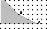
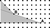
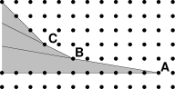
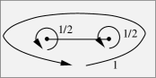
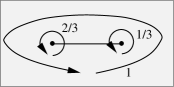
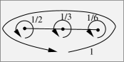
Figure 19: Construction of the line defects with ends and singular points. (Left) - Defect with equivalent ends. (Center) - Defect with inequivalent ends. (Right) - Defect with inequivalent ends and additional singular point splitting defect into two fragments.

Figure 20 demonstrates geometrically modifications which occur with elementary cell after traversing different closed paths on the lattice with $1:2$ defect with two ends. To find the global monodromy one can use elementary $1\times 1$ cell (Fig. 20, left), whereas it is not possible to cross the line with such a cell because of ambiguity of cell modifications.

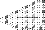
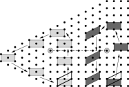
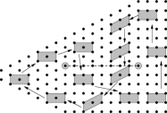
Figure 20: Lattice with two half-integer defects. Defect is an interval with two end points. (Left)- Elementary cell cannot cross unambiguously the defect line. (Center) - Both ends have the same $(1/2)$ monodromy. (Right) - Figure eight close path is not contractible but the monodromy is trivial.

Taking $1\times 2$ cell we can easily go around each singular point and see (Fig. 20, center) that the result is exactly the same for both points, namely the half of the global modifications.

The last Figure 20, (right) shows the evolution of the double cell along the figure eight close path which goes around two centers but in opposite directions. This close path results in trivial monodromy, the cell has no modifications after returning to the initial point.

6 Is there mutual interest in defect - monodromy correspondence?

Stimulated by analogy between classical and quantum monodromy for Hamiltonian integrable systems from one side and defects of regular periodic lattices from another side we have suggested construction of “elementary integer and fractional lattice defects” associated with elementary integer and fractional monodromy. Then we have proposed how to generate more complicated defects of lattices by combination of elementary ones. Among these more complicated defects there are defects like disclinations which are well known in solid state physics. At the same time the author does not know simple examples of dynamical Hamiltonian system with similar defects. Reciprocally, many examples of dynamical Hamiltonian systems with elementary monodromy are known but the “elementary monodromy defect” seems not to be individually detected experimentally in periodic solids. These observations enables us to formulate below a number of problems concerning Hamiltonian dynamical systems with singularities and periodic lattices with defects. Some of these problems have more or less intuitively evident answers but the strict mathematical proofs are still absent. In other cases even the formulation of the problem is not precise and should be critically analyzed and corrected before looking for the answer.

• About the sign of elementary monodromy defect. How to characterize the class of dynamical systems (classical and quantum) possessing only elementary monodromy defects of one sign? For Hamiltonian systems focus-focus singularities correspond to elementary $(-)$ defects. Tentative answer is to say that elementary $(+)$ monodromy defects are generic for $PT$-invariant dynamical systems with non-hermitian Hamiltonians and real spectra Bender ; G24Zhil .

• Correspondence between topology of singular fibers of integrable toric fibrations and integer and fractional defects of lattices. Some simple examples of such correspondence were given. Is it possible to establish more general correspondence? In particular it seems natural that elementary $(+)$ and $(-)$ monodromy defects correspond to pinched tori with different index of transversal self-crossings matsumoto .

• Constructive methods to design Hamiltonian classical and quantum systems with prescribed type of monodromy. Less ambitious task is to propose a list of concrete examples of classical and quantum systems which show the manifestation of different elementary and non-elementary defects.

• Existence of a topological invariant separating different singularities (defects) with the same monodromy but with different numbers of $2\pi$-rotations of elementary cell. The analogy between this problem and the Riemann surfaces description Cartan was pointed out to author on several ocassions.

• Extension of the correspondence between singularities and defects from 2D-systems to higher dimensional systems. This is surely a very wide subject and author believes that first steps in mathematical generalization should be guided by natural physical examples.

• Global restrictions on the system of defects and on the system of singularities of toric fibrations in the case of compact base space (lattices on compact spaces). For example, singular toric fibration over $S^{2}$ base space should have 24 elementary focus-focus singularities zungII or equivalently 24 elementary $(-)$ monodromy defects or 12 $(\pi/3$)-rotational disclinations known as pentagonal defects Nelson83 . This problem has obvious relation with fullerene-like materials.

• The relation between number of removed vertices for a defect and the Duistermaat-Heckman measure for the reduced Hamiltonian system. Hint: The slope of the function giving the number of removed vertices from vertical line as a function of the number of a vertical line coincides with the Chern class of the integrable fibration used in the Duistermaat-Heckman theorem DuistHeck ; Guill .

• To find macroscopic/mesoscopic physical systems which manifest presence of elementary $(+/-)$ monodromy defects. Possible candidates besides periodic solids or liquid crystals may be membranes Bowick01 , fullerenes and curved carbon surfaces ConeNature , viruses SPID , colloidal structures Macromol , etc.

• Relation between internal structure of elementary cells and possible existence of isolated elementary integer and fractional monodromy defects in real physical systems. In what kind of systems (materials) the topological properties are more important than geometric and steric effects and enable one to see the manifestation of elementary monodromy defects?

• Physical consequences of sign conjecture. If one accept the formulated above sign conjecture, i.e. presence of only $(-)$ defects in generic families of Hamiltonian systems depending on a small number of parameters, there is fundamental difference between $(+)$ and $(-)$ (or in other terms between “right” and “left”) in both classical and quantum mechanics. How to formulate this conjecture in more precise terms and what kind of physical consequences can be rigorously deduced?

The author hopes that Hamiltonian dynamics and periodic solids gives complementary points of view which are useful for both fields of scientific interest. The present article is supposed to stimulate mutual interest, better understanding and further cooperation between specialists working in these fields.

Acknowledgements. The author thanks Drs. R. Cushman, N. Nekhoroshev, D. Sadovskii for many stimulating discussions. This work was essentially done during authors stay in IHES, Bures-sur-Yvette, France, Mathematical Institute, Universitty of Warwick, UK, and Max-Planck Institut für Physik komplexer Systeme, Dresden, Germany. The support of these instotutions is acknowledged. This work is a part of the European project MASIE, contract HPRN-CT-2000-00113.

References

- (1) V. I. Arnol’d: Mathematical Methods of Classical Mechanics. Springer, New York, 1981
- (2) L.M. Lerman and Ya. L. Umanskii: Four dimensional integrable Hamiltonian systems with simple singular points, Translations of Mathematical Monographs, 176, AMS, Providence, R.I., 1998.
- (3) N.T. Zung: Diff. Geom. Appl., 7, 123 (1997)
- (4) R.H. Cushman: C.W.I. Newsletter 1, 4 (1983)
- (5) J. J. Duistermaat: Comm. Pure Appl. Math. 33, 687 (1980)
- (6) R. H. Cushman and J. J. Duistermaat: Bull. Am. Math. Soc. 19, 475 (1988)
- (7) L. Bates: J. Appl. Math. Phys. (ZAMP) 42, 837 (1991)
- (8) R.H. Cushman and L.M. Bates: Global aspects of classical integrable systems, Birkhäuser, Basel, 1997.
- (9) D.A. Sadovskii, B.I. Zhilinskii: Phys. Lett. A 256, 235 (1999)
- (10) N.N. Nekhoroshev, D.A. Sadovskii, B.I. Zhilinskii: C. R. Acad. Sci. Paris, Ser. I, 335, 985 (2002)
- (11) Y. Colin de Verdier, S. Vu Ngoc: Ann. Ec. Norm. Sup. in press. (2003)
- (12) N.N. Nekhoroshev, D.A. Sadovskii, B.I. Zhilinskii: in preparation, (2003).
- (13) N. N. Nekhoroshev: Trans. Moscow Math. Soc. 26, 180 (1972)
- (14) L. Grondin, D. A. Sadovskií, and B. I. Zhilinskii: Phys. Rev. A, 142, 012105 (2002)
- (15) S. Vu Ngoc: Comm. Math. Phys. 203, 465 (1999)
- (16) H. Waalkens and H. R. Dullin: Ann. Phys. (N.Y.), 295, 81 (2001)
- (17) M. S. Child, T. Weston, and J. Tennyson: Mol. Phys. 96, 371 (1999)
- (18) M. Kleman: Points Lines and Walls (Chichester: Wiley) 1983.
- (19) N. D. Mermin: Rev. Mod. Phys. 51, 591 (1979)
- (20) L. Michel: Rev. Mod. Phys. 52, 617 (1980)
- (21) E. Kroner: Continuum theory of defects. in Physics of defects. Les Houches, Ecole d’ete de physique theorique. Elsevier, New York. 1981. p. 215-315.
- (22) R. Cushman, S. Vu Ngoc: Ann. I. Henri Poincaré, 3, 883 (2002)
- (23) R. H. Cushman and D. A. Sadovskií: Physica D, 65, 166 (2000)
- (24) V. Matveev: Sb. Math. 187, 495 (1996)
- (25) R. H. Cushman and J. J. Duistermaat: J. Diff. Eqns. 172, 42 (2001).
- (26) V. Arnol’d, A. Avez: Ergodic problems of classical mechanics. Benjamin, New York (1968)
- (27) R. Cushman, B. Zhilinskii: J. Phys. A: Math. Gen 35, L415 (2002)
- (28) C. Bender, S. Boettcher: Phys.Rev. Lett. 80, 5243 (1998)
- (29) B. Zhilinskii: in Proceedings of 24 International Conference on Group-Theoretical Methods in Physics, Paris (2003).
- (30) Y. Matsumoto: J. Math. Soc. Japan 37, 605 (1985)
- (31) E. Cartan: Leçon sur la Géométrie des Espaces de Riemann. (Gauthier-Villars, Paris, 1928) (Chapter 3)
- (32) N.T. Zung: ArXiv:math.DG/0010181 (2001).
- (33) D. R. Nelson: Phys. Rev. B 28, 5515 (1983)
- (34) J. J. Duistermaat, G. J. Heckman: Invent. Math. 69, 259 (1982)
- (35) V. Guillemin: Moment Map and Combinatorial Invariants of Hamiltonian -spaces. (Birkhäuser, Basel, 1994).
- (36) M. J. Bowick, A. Travesset: Phys. Rep. 344, 255 (2001)
- (37) A. Krishnan, et al: Nature, 388, 451 (1997)
- (38) B. K. Ganser et al: Science, 283, 80 (1999)
- (39) S. P. Gido, J. Gunther, E. L. Thomas, D. Hoffman: Macromolecules 26, 4506 (1993)