Three different manifestations
of the quantum Zeno effect

Abstract

Three different manifestations of the quantum Zeno effect are discussed, compared and shown to be physically equivalent. We look at frequent projective measurements, frequent unitary “kicks” and strong continuous coupling. In all these cases, the Hilbert space of the system splits into invariant “Zeno” subspaces, among which any transition is hindered.

1 Introduction

The quantum Zeno phenomenon Misra ; Beskow is usually viewed as the effect of repeated projections von on a quantum system. It is, however, a more general phenomenon, that can be best understood in terms of the dynamical time evolution of quantum systems and fields zenoreview . Indeed, a projection à la von Neumann is just a handy way to “summarize” the complicated physical processes that take place during a quantum measurement. The latter is performed by an external (macroscopic) apparatus and involves complicated interactions with the environment. The external system performing the observation need not be a bona fide detection system, that “clicks” or is endowed with a pointer. It is enough that the information on the state of the observed system be encoded in some external degrees of freedom. Moreover, the interaction between the system and its environment can be fast (as compared to any other timescales involved) or slow. In the former case one says that a “spectral decomposition” à la Wigner takes place Wigner63 ; PN94 [namely a rapid (and unitary) physical process that associates different (external) states to different values of the observable being measured]; in the latter case one says that a “continuous” measurement process occurs Peres80 ; Schulman98 ; zenoreview .

For instance, a spontaneous emission process is often a very effective measurement, for it is irreversible and leads to an entanglement of the state of the system (the emitting atom or molecule) with the state of the apparatus (the electromagnetic field). The von Neumann rules arise when one traces away the photonic state and is left with an incoherent superposition of atomic states. In the light of these observations, it became clear in the 80’s that the main physical features of the Zeno effect would still be apparent if one would formulate the measurement process in more realistic terms, introducing a physical apparatus, a Hamiltonian and a suitable interaction with the measured system, with no explicit use of projection operators.

More to this, once one has realized that the quantum Zeno effect (QZE) is a mere consequence of the dynamics and cannot be ascribed to the “collapse” of the wave function, one would like to understand which features of the dynamical process are essential for observing a QZE. It turns out that not only a bona fide detection scheme, but even irreversibility is unnecessary. In fact, any interactions – and not only those that can be considered as a measurement process of some sort – that considerably affect the system (in a sense to be made more precise in the following) provoke QZE. Therefore, the QZE appears in a much broader context than its original formulation, whenever a strong disturbance dominates the time evolution of the quantum system.

The aim of this article is to discuss three different manifestations of QZE. We start in Sect. 2 with general (projective) measurements, then extend in Sect. 3 the notion of QZE to the case of unitary kicks bang and finally discuss in Sect. 4 (unitary) continuous interactions theorem . We show in Sect. 5 that, in all these cases, the system is forced to evolve in a set of orthogonal (“Zeno”) subspaces of the total Hilbert space. The quantum Zeno subspaces are completely determined by the disturbance: they are nothing but its invariant subspaces; in the two latter cases (unitary kicks and continuous coupling) they are the eigenspaces of the interaction. An example is considered in Sect. 6 and discussed in Sect. 7. We conclude with a rapid overlook in Sect. 8.

2 Projective measurements

We first consider the case of bona fide measurements, described by projection operators à la von Neumann von . The measurements are in general:

• “incomplete,” in the sense that some outcomes may be lumped together (for instance because the measuring apparatus has insufficient resolution); this means that the projection operator that selects a particular lump is multidimensional (and in this sense the information gained on the measured observable is incomplete);

• “nonselective,” in the sense that the measuring apparatus does not select the different outcomes, but simply destroys the phase correlations between some states, provoking the transition from a pure state to a mixture.

See, for example, Schwinger59 ; Peres98 .

Let us outline the extension theorem of Misra and Sudarshan’s theorem Misra on the QZE to the case of incomplete and nonselective measurements. Let Q be a quantum system, whose states belong to the Hilbert space ${\cal H}$ and whose evolution is described by the superoperator

$$\hat{U}_{t}\rho=U(t)\rho U^{\dagger}(t),\qquad U(t)=\exp(-iHt)$$ (1)

where $\rho$ is the density matrix of the system and $H$ a time-independent lower-bounded Hamiltonian. Let

$$\{P_{n}\}_{n},\qquad P_{n}P_{m}=\delta_{mn}P_{n},\qquad\sum_{n}P_{n}=1,$$ (2)

be an orthogonal resolution of the identity and $P_{n}{\mathcal{H}}={\mathcal{H}}_{n}$ the relative subspaces. The associated partition on the total Hilbert space is

$${\mathcal{H}}=\bigoplus_{n}{\mathcal{H}}_{n}.$$ (3)

The nonselective measurement is described by the superoperator

$$\hat{P}\rho=\sum_{n}P_{n}\rho P_{n}$$ (4)

and the evolution after $N$ measurements in a time $t$ is governed by the superoperator

$$\hat{V}^{(N)}_{t}=\underbrace{\left(\hat{P}\hat{U}_{t/N}\right)\left(\hat{P}\hat{U}_{t/N}\right)\cdots\left(\hat{P}\hat{U}_{t/N}\right)}_{N\mathrm{times}}=\left(\hat{P}\hat{U}_{t/N}\right)^{N}.$$ (5)

We perform a first, preparatory measurement, so that the initial state is

$$\hat{P}\rho_{0}=\sum_{n}P_{n}\rho_{0}P_{n}.$$ (6)

By assuming the time-reversal invariance and the existence of the strong limits ($t>0$)

$${\mathcal{V}}_{n}(t)=\lim_{N\to\infty}\left[P_{n}U\left(\frac{t}{N}\right)\right]^{N},\qquad\lim_{t\rightarrow 0^{+}}{\mathcal{V}}_{n}(t)=P_{n},\quad\forall n\$$ (7)

one can show that the operators ${\mathcal{V}}_{n}(t)$ exist for all real $t$ and form a semigroup and that the final state, engendered by the limiting superoperator

$$\hat{\mathcal{V}}_{t}\equiv\lim_{N\to\infty}\hat{V}^{(N)}_{t},$$ (8)

is

$$\rho(t)=\hat{\mathcal{V}}_{t}\rho_{0}=\sum_{n}{\mathcal{V}}_{n}(t)\rho_{0}{\mathcal{V}}_{n}^{\dagger}(t),\quad\mathrm{with}\quad\sum_{n}{\mathcal{V}}_{n}^{\dagger}(t){\mathcal{V}}_{n}(t)=\sum_{n}P_{n}=\mathbf{1}.\;\;$$ (9)

The components ${\mathcal{V}}_{n}(t)\rho_{0}{\mathcal{V}}_{n}^{\dagger}(t)$ make up a block diagonal matrix: the initial density matrix is reduced to a mixture and any interference between different subspaces ${\mathcal{H}}_{n}$ is destroyed (complete decoherence). Moreover,

$$p_{n}(t)=\mathrm{Tr}\left[\rho(t)P_{n}\right]=\mathrm{Tr}\left[{\mathcal{V}}_{n}(t)\rho_{0}{\mathcal{V}}_{n}^{\dagger}(t)\right]=\mathrm{Tr}\left[\rho_{0}P_{n}\right]=p_{n}(0),\quad\forall n.$$ (10)

In words, probability is conserved in each subspace and no probability “leakage” between any two subspaces is possible: the total Hilbert space splits into invariant “Zeno” subspaces ${\mathcal{H}}_{n}$ and the different components of the density matrix evolve independently within each sector. One can think of the total Hilbert space as the shell of a tortoise, each invariant subspace being one of the scales. Motion among different scales is impossible. (See Fig. 1 in the following.) Misra and Sudarshan’s seminal result is reobtained when $p_{n}(0)=1$ for some $n$, in (10): the initial state is then in one of the invariant subspaces and the survival probability in that subspace remains unity.

An important particular case is when the Hamiltonian is bounded $\|H\|<\infty$. Then each limiting evolution operator ${\mathcal{V}}_{n}(t)$ in (7) is unitary within the subspace ${\mathcal{H}}_{n}$ and has the form

$${\mathcal{V}}_{n}(t)=\lim_{N\to\infty}[P_{n}U(t/N)P_{n}]^{N}=P_{n}\exp(-iP_{n}HP_{n}t).$$ (11)

More generally, if ${\mathcal{H}}_{n}\subset D(H)$ (which is trivially satisfied for a bounded $H$), then the resulting Hamiltonian $P_{n}HP_{n}$ is self-adjoint and ${\mathcal{V}}_{n}(t)$ is unitary in ${\mathcal{H}}_{n}$. When the above condition does not hold, one can always formally write the limiting evolution in the form (11), but has to define the meaning of $P_{n}HP_{n}$ and study the self-adjointness of the limiting Hamiltonian $P_{n}HP_{n}$ Friedman72 ; compactregularize .

In any case, with the necessary precautions on the meaning of operators and boundary conditions, the Zeno evolution can be written

$${\mathcal{V}}_{n}(t)=P_{n}\exp(-iH_{\mathrm{Z}}t)$$ (12)

where

$$H_{\mathrm{Z}}=\hat{P}H=\sum_{n}P_{n}HP_{n}$$ (13)

is the “Zeno” Hamiltonian.

3 Unitary kicks

The formulation of the preceding section hinges upon projections à la von Neumann. Projections are (supposed to be) instantaneous processes, yielding the collapse of the wave function (an ultimately nonunitary process). However, one can obtain the QZE without making use of nonunitary evolutions PN94 , by exploiting Wigner’s idea of spectral decomposition Wigner63 . In this section we further elaborate on this issue, obtaining the QZE by means of a generic sequence of frequent instantaneous unitary processes, that need not be spectral decompositions. We will only give the main results, as additional details and a complete proof, which is related to von Neumann’s ergodic theorem ReedSimon , can be found in bang .

Consider the dynamics of a quantum system Q undergoing $N$ “kicks” $U_{\mathrm{kick}}$ (instantaneous unitary transformations) in a time interval $t$

$$U_{N}(t)=\underbrace{\left[U_{\mathrm{kick}}U\left(\frac{t}{N}\right)\right]\left[U_{\mathrm{kick}}U\left(\frac{t}{N}\right)\right]\cdots\left[U_{\mathrm{kick}}U\left(\frac{t}{N}\right)\right]}_{N\mathrm{times}}.$$ (14)

In the large $N$ limit, the dominant contribution is $U_{\mathrm{kick}}^{N}$. One therefore considers the sequence of unitary operators

$$V_{N}(t) = U_{\mathrm{kick}}^{\dagger N}U_{N}(t)=U_{\mathrm{kick}}^{\dagger N}\left[U_{\mathrm{kick}}U\left(\frac{t}{N}\right)\right]^{N}$$ (15)

and its limit

$${\mathcal{U}}(t)\equiv\lim_{N\to\infty}V_{N}(t).$$ (16)

One can show that

$${\mathcal{U}}(t)=\exp(-iH_{\mathrm{Z}}t),$$ (17)

where

$$H_{\mathrm{Z}}=\hat{P}H=\sum_{n}P_{n}HP_{n}$$ (18)

is the Zeno Hamiltonian, $P_{n}$ being the spectral projections of $U_{\mathrm{kick}}$

$$U_{\mathrm{kick}}=\sum_{n}e^{-i\lambda_{n}}P_{n}.\quad(e^{-i\lambda_{n}}\neq e^{-i\lambda_{l}},\;\mbox{for}\;n\neq l)$$ (19)

Incidentally, notice that in this case the map $H_{\mathrm{Z}}=\hat{P}H$ is the projection onto the centralizer (commutant)

$$Z(U_{\mathrm{kick}})=\{X|\;[X,U_{\mathrm{kick}}]=0\}.$$ (20)

In conclusion

$$U_{N}(t)\sim U_{\mathrm{kick}}^{N}{\mathcal{U}}(t)=U_{\mathrm{kick}}^{N}\exp(-iH_{\mathrm{Z}}t)=\exp\left(-i\sum_{n}N\lambda_{n}P_{n}+P_{n}HP_{n}t\right).$$ (21)

(22)

The unitary evolution (14) yields therefore a Zeno effect and a partition of the Hilbert space into Zeno subspaces, like in the case of repeated projective measurements discussed in Sect. 2. The appearance of the Zeno subspaces is a direct consequence of the wildly oscillating phases between different eigenspaces of the kick and hinges upon a mean ergodic theorem. This is equivalent to a procedure of randomization of the phases. We will see a similar situation in the next section, in terms of a strong continuous coupling. Notice that if a projection is viewed as a shorthand notation for a spectral decomposition Wigner63 ; PN94 , the above dynamical scheme includes, for all practical purposes, the usual formulation of the quantum Zeno effect in terms of projection operators.

It is superfluous to stress the analogy of the approach outlined in this section with the seminal papers on quantum maps and quantum chaos qch . In this context, see varieidee .

4 Continuous coupling

The formulation of the preceding sections hinges upon instantaneous processes, that can be unitary or nonunitary. However, as explained in the introduction, the basic features of the QZE can be obtained by making use of a continuous coupling, when the external system takes a sort of steady “gaze” at the system of interest. The mathematical formulation of this idea is contained in a theorem thesis ; theorem on the (large-$K$) dynamical evolution governed by a generic Hamiltonian of the type

$$H_{K}=H+KH_{\mathrm{c}},$$ (23)

which again need not describe a bona fide measurement process. $H$ is the Hamiltonian of the quantum system investigated and $H_{\mathrm{c}}$ can be viewed as an “additional” interaction Hamiltonian performing the “measurement.” $K$ is a coupling constant.

Consider the time evolution operator

$$U_{K}(t)=\exp(-iH_{K}t).$$ (24)

In the “infinitely strong measurement” (“infinitely quick detector”) limit $K\to\infty$, the dominant contribution is $\exp(-iKH_{\mathrm{c}}t)$. One therefore considers the limiting evolution operator

$${\mathcal{U}}(t)=\lim_{K\to\infty}\exp(iKH_{\mathrm{c}}t)\,U_{K}(t),$$ (25)

that can be shown to have the form

$${\mathcal{U}}(t)=\exp(-iH_{\mathrm{Z}}t),$$ (26)

where

$$H_{\mathrm{Z}}=\hat{P}H=\sum_{n}P_{n}HP_{n}$$ (27)

is the Zeno Hamiltonian [projection of the system Hamiltonian $H$ onto the centralizer $Z(H_{\mathrm{c}})$], $P_{n}$ being the eigenprojection of $H_{\mathrm{c}}$ belonging to the eigenvalue $\eta_{n}$

$$H_{\mathrm{c}}=\sum_{n}\eta_{n}P_{n},\qquad(\eta_{n}\neq\eta_{m},\quad\mbox{for}\;n\neq m)\ .$$ (28)

This is formally identical to (13) and (18). In conclusion, the limiting evolution operator is

$$U_{K}(t)\sim\exp(-iKH_{\mathrm{c}}t)\,{\mathcal{U}}(t)=\exp\left(-i\sum_{n}Kt\eta_{n}P_{n}+P_{n}HP_{n}t\right),$$ (29)

whose block-diagonal structure is explicit. Compare with (22). The above statements can be proved by making use of the adiabatic theorem Messiah61 . It is also worth emphasizing interesting links with the quantum evolution in the strong coupling limit Frasca .

The idea of formulating the Zeno effect in terms of a “continuous coupling” to an external apparatus has often appeared in the literature of the last two decades Peres80 ; varicont . However, the first quantitative estimate of the link with the formulation in terms of projective measurements is rather recent Schulman98 (see also zenoreview ).

5 Dynamical superselection rules

Let us briefly consider the main physical implications. In the $N\to\infty$ ($K\to\infty$) limit the time evolution operator ${\mathcal{U}}(t)$ becomes diagonal with respect to $U_{\mathrm{kick}}$ or $H_{\mathrm{c}}$,

$$[{\mathcal{U}}(t),U_{\mathrm{kick}}]=0,\qquad[{\mathcal{U}}(t),H_{\mathrm{c}}]=0,$$ (30)

a superselection rule arises and the total Hilbert space is split into subspaces ${\mathcal{H}}_{n}$ which are invariant under the evolution. The dynamics within each Zeno subspace ${\mathcal{H}}_{n}$ is essentially governed by the diagonal part $H_{\mathrm{Z}}P_{n}=P_{n}HP_{n}$ of the system Hamiltonian $H$ [the remaining part of the evolution consisting in a sector-dependent phase] and the probability to find the system in each ${\mathcal{H}}_{n}$

$$p_{n}(t) = \mathrm{Tr}\left[\rho(t)P_{n}\right]=\mathrm{Tr}\left[{\mathcal{U}}(t)\rho_{0}{\mathcal{U}}^{\dagger}(t)P_{n}\right]=\mathrm{Tr}\left[{\mathcal{U}}(t)\rho_{0}P_{n}{\mathcal{U}}^{\dagger}(t)\right]$$ (31)

$$= \mathrm{Tr}\left[\rho_{0}P_{n}\right]=p_{n}(0)$$ (32)

is constant. As a consequence, if the initial state is an incoherent superposition of the form (6), then each component will evolve separately, according to

$$\rho(t)={\mathcal{U}}(t)\rho_{0}{\mathcal{U}}^{\dagger}(t)=\sum_{n}{\mathcal{V}}_{n}(t)\rho_{0}{\mathcal{V}}_{n}^{\dagger}(t),$$ (33)

with ${\mathcal{V}}_{n}(t)=P_{n}\exp(-iP_{n}HP_{n}t)$, which is exactly the same result (9)-(11) found in the case of projective measurements. In Fig. 1 we endeavored to give a pictorial representation of the decomposition of the Hilbert space in the three cases discussed (projective measurements, kicks and continuous coupling).

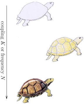
Figure 1: The Hilbert space of the system: a dynamical superselection rule appears as the number of measurements $N$ or the number of kicks $N$ or the coupling $K$ to the apparatus are increased

Notice, however, that there is one important difference between the nonunitary evolution discussed in Sect. 2 and the dynamical evolution discussed in Sects. 3-4: indeed, if the initial state $\rho_{0}$ contains coherent terms between any two Zeno subspaces ${\mathcal{H}}_{n}$ and ${\mathcal{H}}_{m}$, $P_{n}\rho_{0}P_{m}\neq 0$, these vanish after the first projection (9) in Sect. 2: $P_{n}\rho(0^{+})P_{m}=0$ [the state becomes an incoherent superposition $\rho(0^{+})\neq\rho_{0}$, whence $\mathrm{Tr}\rho(0^{+})^{2}<\mathrm{Tr}\rho_{0}^{2}$]. On the other hand, such terms are preserved by dynamical (unitary) evolution analyzed in Sects. 3-4, and do not vanish, even though they wildly oscillate. For example, consider the initial state

$$\rho_{0}=(P_{n}+P_{m})\rho_{0}(P_{n}+P_{m}),\qquad P_{n}\rho_{0}P_{m}\neq 0.$$ (34)

By (22) and (29) it evolves into

$$\rho(t) = {\mathcal{V}}_{n}(t)\rho_{0}{\mathcal{V}}^{\dagger}_{n}(t)+{\mathcal{V}}_{m}(t)\rho_{0}{\mathcal{V}}^{\dagger}_{m}(t)$$ (36)

$$+\;e^{-iN(\lambda_{n}-\lambda_{m})}{\mathcal{V}}_{n}(t)\rho_{0}{\mathcal{V}}^{\dagger}_{m}(t)+e^{iN(\lambda_{n}-\lambda_{m})}{\mathcal{V}}_{m}(t)\rho_{0}{\mathcal{V}}^{\dagger}_{n}(t),$$

$$\rho(t) = {\mathcal{V}}_{n}(t)\rho_{0}{\mathcal{V}}^{\dagger}_{n}(t)+{\mathcal{V}}_{m}(t)\rho_{0}{\mathcal{V}}^{\dagger}_{m}(t)$$ (38)

$$+\;e^{-iK(\eta_{n}-\eta_{m})t}{\mathcal{V}}_{n}(t)\rho_{0}{\mathcal{V}}^{\dagger}_{m}(t)+e^{iK(\eta_{n}-\eta_{m})t}{\mathcal{V}}_{m}(t)\rho_{0}{\mathcal{V}}^{\dagger}_{n}(t),$$

respectively, at variance with (9) and (33), respectively. Therefore $\mathrm{Tr}\rho(t)^{2}=\mathrm{Tr}\rho_{0}^{2}$ for any $t$ and the Zeno dynamics is unitary in the whole Hilbert space ${\mathcal{H}}$. We notice that these coherent terms become unobservable in the large-$N$ or large-$K$ limit, as a consequence of the Riemann-Lebesgue theorem (applied to any observable that “connects” different sectors and whose time resolution is finite). This interesting aspect is reminiscent of some results on “classical” observables Jauch , semiclassical limit Berry and quantum measurement theory Araki ; Schwinger59 .

It is worth noticing that the superselection rules discussed here are de facto equivalent to the celebrated “W³” ones WWW , but turn out to be a mere consequence of the Zeno dynamics. For a related discussion, but in a different context, see Giulini .

6 An example

One of the main potential applications of the quantum Zeno subspaces concerns the possibility of “freezing” the loss of quantum mechanical coherence and probability leakage due to the interaction of the system of interest with its environment. Let us therefore look at an elementary example in the light of the three different formulations of the Zeno effect summarized in Sections 2-4. In the following, it can be helpful to think of the Zeno subspace ${\mathcal{H}}_{1}$ as the quantum computation subspace (qubit) that one wants to protect from decoherence.

Consider a 3-level system in ${\mathcal{H}}_{\mathrm{sys}}=\mathbb{C}^{3}$

$$\langle a|=(1,0,0),\quad\langle b|=(0,1,0),\quad\langle c|=(0,0,1)$$ (39)

and the Hamiltonian

$$H=\Omega_{1}(|a\rangle\langle b|+|b\rangle\langle a|)+\Omega_{2}(|b\rangle\langle c|+|c\rangle\langle b|)=\pmatrix{0&\Omega_{1}&0\cr\Omega_{1}&0&\Omega_{2}\cr 0&\Omega_{2}&0}.$$ (40)

We perform the (incomplete, nonselective) projective measurements ($P_{1}+P_{2}=\mathbf{1}$)

$$P_{1}=|a\rangle\langle a|+|b\rangle\langle b|=\pmatrix{1&0&0\cr 0&1&0\cr 0&0&0},\quad P_{2}=|c\rangle\langle c|=\pmatrix{0&0&0\cr 0&0&0\cr 0&0&1},$$ (41)

yielding the partition (3), with $\mathrm{dim}{\mathcal{H}}_{1}=2$, $\mathrm{dim}{\mathcal{H}}_{2}=1$. The evolution operators (11) read

$${\mathcal{V}}_{1} =P_{1}\exp(-iP_{1}HP_{1}t) =P_{1}\exp\left[-i\pmatrix{0&\Omega_{1}t&0\cr\Omega_{1}t&0&0\cr 0&0&0}\right]$$ (43)

$$=\pmatrix{\cos\Omega_{1}t&-i\sin\Omega_{1}t&0\cr-i\sin\Omega_{1}t&\cos\Omega_{1}t&0\cr 0&0&0},$$

$${\mathcal{V}}_{2} =P_{2}\exp(-iP_{2}HP_{2}t) =P_{2}=\pmatrix{0&0&0\cr 0&0&0\cr 0&0&1}$$ (44)

and the Zeno Hamiltonian (13) is

$$H_{\mathrm{Z}}=P_{1}HP_{1}+P_{2}HP_{2}=\pmatrix{0&\Omega_{1}&0\cr\Omega_{1}&0&0\cr 0&0&0}.$$ (45)

The initial state (6) evolves according to (9): in the Zeno limit ($N\to\infty$), the subspaces ${\mathcal{H}}_{1}$ and ${\mathcal{H}}_{2}$ decouple. If the coupling $\Omega_{2}$ is viewed as a caricature of the loss of quantum mechanical coherence, the subspace ${\mathcal{H}}_{1}$ becomes “decoherence free” Viola99 . See Fig. 2.

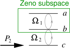
Figure 2: Three level system undergoing measurements ($P_{1}$ not indicated). We explicitly showed the Zeno subspace ${\mathcal{H}}_{1}$

In order to understand how unitary kicks yield the Zeno subspaces, consider the 4-level system in the enlarged Hilbert space ${\mathcal{H}}_{\mathrm{sys}}\oplus\mathrm{span}\{|M\rangle\}$

$$\langle a|=(1,0,0,0),\quad\langle b|=(0,1,0,0),\quad\langle c|=(0,0,1,0),\quad\langle M|=(0,0,0,1)$$ (46)

and the Hamiltonian

$$H=\Omega_{1}(|a\rangle\langle b|+|b\rangle\langle a|)+\Omega_{2}(|b\rangle\langle c|+|c\rangle\langle b|)=\pmatrix{0&\Omega_{1}&0&0\cr\Omega_{1}&0&\Omega_{2}&0\cr 0&\Omega_{2}&0&0\cr 0&0&0&0}.$$ (47)

This is the same example as (39)-(40), but we added a fourth level $|M\rangle$. We now couple $|M\rangle$ to $|c\rangle$ by performing the unitary kicks

$$U_{\mathrm{kick}} = e^{-i\lambda_{1}}P_{1}+e^{-i\lambda_{2}(|c\rangle\langle M|+|M\rangle\langle c|)}=\pmatrix{e^{-i\lambda_{1}}&0&0&0\cr 0&e^{-i\lambda_{1}}&0&0\cr 0&0&\cos\lambda_{2}&-i\sin\lambda_{2}\cr 0&0&-i\sin\lambda_{2}&\cos\lambda_{2}}$$ (48)

$$= \sum_{n=1,\pm}e^{-i\lambda_{n}}P_{n},$$ (49)

where $\lambda_{1}\neq\lambda_{2}=\lambda_{+}=-\lambda_{-}\neq\lambda_{1}$ (otherwise arbitrary), and the subspaces are defined by

$$\halign to=433.62pt{\@eqnsel\hskip\@centering$\displaystyle{#}$&\global\@eqcnt\@ne\hskip 2\arraycolsep\hfil${#}$\hfil&\global\@eqcnt\tw@\hskip 2\arraycolsep$\displaystyle{#}$\hfil&\llap{#}\cr\hfil\hskip 0.0pt plus 1000.0pt$\displaystyle{P_{1} &10.0pt\hfil${=&10.0pt$\displaystyle{| a \rangle \langle a | + | b \rangle \langle b |= \pmatrix{1 &0 &0 &0\cr 0 &1 &0 &0 \cr 0 &0 &0 &0 \cr 0 &0 &0 &0 } , {}&\hbox to0.0pt{\hss{\rm(0.50a)}\cr\penalty 100\vskip 3.0pt\vskip 0.0pt\cr\hfil\hskip 0.0pt plus 1000.0pt$\displaystyle{P_{\pm}&10.0pt\hfil${=&10.0pt$\displaystyle{\frac{(| c \rangle \pm| M \rangle)(\langle c | \pm\langle M |)}{2} = \frac{1}{2}\pmatrix{0 &0 &0 &0\cr 0 &0 &0 &0 \cr 0 &0 &1 &\pm 1 \cr 0 &0 &\pm 1 &1 } . &\hbox to0.0pt{\hss{\rm(0.50b)}\cr}}}}}}}}}$$

($P_{1}+P_{-}+P_{+}=\mathbf{1}$.)

Figure 3: Three level system undergoing frequent unitary kicks that couple one of its levels to an “external” system $M$. ($\lambda_{1}=0$.) We explicitly indicated the Zeno subspace ${\mathcal{H}}_{1}$

In the Zeno limit ($N\to\infty$) the subspaces ${\mathcal{H}}_{1}$, ${\mathcal{H}}_{+}$ and ${\mathcal{H}}_{-}$ decouple due to the wildly oscillating phases O$(N)$. See Fig. 3. The Zeno Hamiltonian (18) reads

$$H_{\mathrm{Z}}=\sum_{n}P_{n}HP_{n}=\pmatrix{0&\Omega_{1}&0&0\cr\Omega_{1}&0&0&0\cr 0&0&0&0\cr 0&0&0&0}$$ (51)

and the evolution (22) is

$$U_{N}(t) \sim \exp\left(-i\sum_{n}N\lambda_{n}P_{n}+P_{n}HP_{n}t\right)$$ (52)

$$= \exp\left[-i\pmatrix{N\lambda_{1}&\Omega_{1}t&0&0\cr\Omega_{1}t&N\lambda_{1}&0&0\cr 0&0&0&N\lambda_{2}\cr 0&0&N\lambda_{2}&0}\right].$$ (53)

A natural choice, yielding no phases in the (Zeno) subspace of interest, is $\lambda_{1}=0,\lambda_{2}=1$:

$$U_{N}(t) \sim \exp\left[-i\pmatrix{0&\Omega_{1}t&0&0\cr\Omega_{1}t&0&0&0\cr 0&0&0&N\cr 0&0&N&0}\right]$$ (54)

$$= \pmatrix{\cos\Omega_{1}t&-i\sin\Omega_{1}t&0&0\cr-i\sin\Omega_{1}t&\cos\Omega_{1}t&0&0\cr 0&0&\cos N&-i\sin N\cr 0&0&-i\sin N&\cos N}.$$ (55)

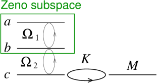
Figure 4: Three level system with one of its levels strongly coupled to an “external” system $M$. We explicitly indicated the Zeno subspace ${\mathcal{H}}_{1}$

Finally, in order to understand how the scheme involving continuous measurements works, add to (47) the Hamiltonian (acting on ${\mathcal{H}}_{\mathrm{sys}}\oplus\mathrm{span}\{|M\rangle\}$)

$$KH_{\mathrm{c}}=K(|c\rangle\langle M|+|M\rangle\langle c|)=\pmatrix{0&0&0&0\cr 0&0&0&0\cr 0&0&0&K\cr 0&0&K&0}=K\left(P_{+}-P_{-}\right)\;,$$ (56)

where $P_{\pm}$ are the same as in (6). The fourth level $|M\rangle$ is now “continuously” coupled to level $|c\rangle$, $K\in\mathbb{R}$ being the strength of the coupling Militello01 . As $K$ is increased, level $|M\rangle$ performs a better “continuous observation” of $|c\rangle$, yielding the Zeno subspaces. The eigenprojections of $H_{\mathrm{c}}$ [see (28)]

$$H_{\mathrm{c}}=\eta_{1}P_{1}+\eta_{-}P_{-}+\eta_{+}P_{+}$$ (57)

are again (6)-(6), with $\eta_{1}=0,\eta_{\pm}=\pm 1$. Once again, in the Zeno limit ($K\to\infty$) the subspaces ${\mathcal{H}}_{1}$, ${\mathcal{H}}_{+}$ and ${\mathcal{H}}_{-}$ decouple due to the wildly oscillating phases O$(K)$. See Fig. 4. The Zeno Hamiltonian $H_{\mathrm{Z}}$ is given by (27) and turns out to be identical to (51), while the evolution (29) explicitly reads

$$U_{K}(t) \sim \exp\left(-i\sum_{n}Kt\eta_{n}P_{n}+P_{n}HP_{n}t\right)$$ (58)

$$= \exp\left[-i\pmatrix{0&\Omega_{1}t&0&0\cr\Omega_{1}t&0&0&0\cr 0&0&0&Kt\cr 0&0&Kt&0}\right]$$ (59)

$$= \pmatrix{\cos\Omega_{1}t&-i\sin\Omega_{1}t&0&0\cr-i\sin\Omega_{1}t&\cos\Omega_{1}t&0&0\cr 0&0&\cos Kt&-i\sin Kt\cr 0&0&-i\sin Kt&\cos Kt}.$$ (60)

[Compare with (55): $Kt$ plays the role of $N$.] It is interesting to notice that with our choice $\eta_{1}=0$ there are no spurious phases in the (Zeno) subspace of interest.

7 More examples

7.1 Simplified scheme

Level $|M\rangle$ and the enlarged Hilbert space ${\mathcal{H}}_{\mathrm{sys}}\oplus\mathrm{span}\{|M\rangle\}$ are not necessary for our discussion. They were introduced in the example of the previous section only for the sake of clarity. Consider, instead of (49), the kicks in the original Hilbert space ${\mathcal{H}}_{\mathrm{sys}}=\mathbb{C}^{3}$

$$U_{\mathrm{kick}}^{\prime}=e^{-i\lambda_{1}}P_{1}+e^{-i\lambda_{2}}P_{2},\quad(e^{-i\lambda_{1}}\neq e^{-i\lambda_{2}})$$ (61)

performed on the three-level system (39)-(41). A straightforward analysis yields, in the Zeno limit $N\to\infty$, the decomposition ${\mathcal{H}}_{1}\oplus{\mathcal{H}}_{2}$. In addition, if $\lambda_{1}=0,\lambda_{2}=1$, then

$$U_{\mathrm{kick}}^{\prime}=P_{1}+e^{-i}P_{2}=e^{-iP_{2}}=e^{-i|c\rangle\langle c|}$$ (62)

and no spurious phases appear.

Analogously, consider instead of (56), the Hamiltonian in ${\mathcal{H}}_{\mathrm{sys}}$

$$H_{\mathrm{c}}^{\prime}=\eta_{1}P_{1}+\eta_{2}P_{2}\quad(\eta_{1}\neq\eta_{2})$$ (63)

added to (40) in the three-level scheme (39)-(41). One obtains again, in the $N\to\infty$ limit, the decomposition ${\mathcal{H}}_{1}\oplus{\mathcal{H}}_{2}$. In addition, if $\eta_{1}=0$ and $\eta_{2}=1$, then

$$H_{\mathrm{c}}^{\prime}=P_{2}=|c\rangle\langle c|$$ (64)

(a very simple situation) and no fast oscillating phases appear.

7.2 Spontaneous decay in vacuum

As we explained in the previous section, one of the most interesting potential applications of the quantum Zeno subspaces concerns the possibility of freezing decoherence, viewed as loss of phase correlation and/or probability leakage to the environment. The model outlined in the previous section is too simple to schematize a genuine decoherence process. For instance, take (47)+(56), exemplified in Fig. 4: the continuous coupling $K$ does not freeze the decay of level $|b\rangle$ onto level $|c\rangle$, it simply hinders the Rabi transition $|b\rangle\leftrightarrow|c\rangle$. A better model would be

$$H_{K}=H_{\mathrm{decay}}+KH_{\mathrm{c}}=\pmatrix{0&\Omega_{1}&0&0\cr\Omega_{1}&0&\tau_{\mathrm{Z}}^{-1}&0\cr 0&\tau_{\mathrm{Z}}^{-1}&-i2/\tau_{\mathrm{Z}}^{2}\gamma&K\cr 0&0&K&0}.$$ (65)

This describes the spontaneous emission of level $|b\rangle$ into a (structured) continuum, which in turn is resonantly coupled to a fourth level $|M\rangle$ zenoreview . The quantity $\gamma$ represents the decay rate to the continuum and $\tau_{\mathrm{Z}}=\Omega_{2}^{-1}$ is the Zeno time hydrogen (convexity of the initial quadratic region). Notice, incidentally, that the Zeno time can be consistently defined also for open quantum systems BenFlor .

This case is relevant for quantum computation, if one is interested in protecting a given subspace (${\mathcal{H}}_{1}$) from decoherence, by inhibiting spontaneous emission. A somewhat related example is considered in Agarwal01 . A proper analysis of this model yields to the following main conclusions: as expected, when the Rabi frequency $K$ is increased, the spontaneous emission from level $|b\rangle$ (to be “protected” from decay/decoherence) is hindered. However, the real problem are the relevant timescales: in order to get an effective “protection” of level $|b\rangle$, one needs $K>1/\tau_{\mathrm{Z}}$. More to this, if the decaying state $|b\rangle$ has energy $\omega_{b}\neq 0$, an inverse Zeno effect antiZeno ; heraclitus may take place and the requirement for obtaining the QZE becomes even more stringent heraclitus , yielding $K>1/\tau_{\mathrm{Z}}^{2}\gamma$. Both these conditions can be very demanding for a real system subject to dissipation. For instance, typical values for spontaneous decay in vacuum are $\gamma\simeq 10^{9}$s^-1, $\tau_{\mathrm{Z}}^{2}\simeq 10^{-29}$s² and $1/\tau_{\mathrm{Z}}^{2}\gamma\simeq 10^{20}$s^-1 hydrogen . The situation can be made more favorable by using cavities. In this context, model (65) yields some insights in the examples analyzed in Viola99 and Beige00 , but we will not further elaborate on this point here.

We emphasize that the case considered in this subsection is not to be regarded as a toy model. The numerical figures we have given are realistic and the Hamiltonian (65) is a good approximation of the decay process at short (for the physical meaning of “short”, see zenoreview ; heraclitus ; Antoniou ) and intermediate times (it is not valid for very large times, where a power law should appear). Related interesting proposals, making use of kicks or continuous coupling in cavity QED, can be found in Qcomp . We stress, once again, that the key issue to address is that of the physically relevant numerical figures and timescales.

7.3 Decohering levels

The example analyzed in Sect. 6 essentially aimed at clarifying that the dynamics in a given subspace ${\mathcal{H}}_{1}=\mathrm{span}\{|a\rangle,|b\rangle\}$ can be decoupled from the dynamical evolution in the total space. However, it is worth stressing that level $|a\rangle$ played no role in our discussion. As a matter of fact, level $|a\rangle$ was simply introduced for convenience, as only level $|b\rangle$ was interacting with other levels/systems. Clearly, in a more general framework, one should look at the decoherence effects on all levels that are coupled to other systems and/or to the environment.

8 Outlook

We have endeavored to clarify that the main physical features of the quantum Zeno effect are not peculiar to a quantum measurement process, but can be framed in a much broader context if one replaces the projections by a suitable (kicked or continuous) interaction of the system under investigation (possibly with an apparatus). However, obviously, whenever the interaction describes a bona fide measurement process performed by a physical apparatus, one can make use of projection operators à la von Neumann, if such a description turns out to be simpler and more economic. This is the principle of Occam’s razor.

A number of important issues have not been discussed in the present article. Among these, the reach and practical importance of the experiments on the QZE expts ; Wilkinson ; Itanodisc and the physical meaning of the mathematical expressions “$N\to\infty$” and “$K\to\infty$” heraclitus ; zenoreview , that may involve delicate quantum field theoretical issues QFT . We will not elaborate on this here, but warn the reader that the expression “large $N$” and “large $K$” should not be taken lightheartedly, as they are directly related to the physically relevant timescales characterizing the evolution. This is the key issue to address, in view of possible applications.

References

- (1) B. Misra, E.C.G. Sudarshan: J. Math. Phys. 18, 756 (1977)
- (2) A. Beskow, J. Nilsson: Arkiv für Fysik 34, 561 (1967); L.A. Khalfin: JETP Letters 8, 65 (1968)
- (3) J. von Neumann: Mathematical Foundation of Quantum Mechanics (Princeton University Press, Princeton, 1955); G. Lüders: Ann. Phys. (Leipzig) 8, 322 (1951)
- (4) P. Facchi, S. Pascazio: Progress in Optics, ed. by E. Wolf (Elsevier, Amsterdam, 2001), Vol. 42, Ch. 3, p. 147
- (5) E.P. Wigner: Am. J. Phys. 31, 6 (1963)
- (6) S. Pascazio, M. Namiki: Phys. Rev. A 50, 4582 (1994)
- (7) A. Peres: Am. J. Phys. 48, 931 (1980); K. Kraus: Found. Phys. 11, 547 (1981); A. Sudbery: Ann. Phys. 157, 512 (1984)
- (8) L.S. Schulman: Phys. Rev. A 57, 1509 (1998)
- (9) P. Facchi, D.A. Lidar, S. Pascazio, ‘Generalized dynamical decoupling from the quantum Zeno effect’, quant-ph/0303132 (2003)
- (10) P. Facchi, S. Pascazio: Phys. Rev. Lett. 89, 080401 (2002)
- (11) J. Schwinger: Proc. Nat. Acad. Sc. 45, 1552 (1959); Quantum kinematics and dynamics (Perseus Publishing, New York, 1991)
- (12) A. Peres: Quantum Theory: Concepts and Methods (Kluwer Academic Publishers, Dordrecht, 1998)
- (13) C.N. Friedman: Indiana Univ. Math. J. 21, 1001 (1972); K. Gustafson: ‘Irreversibility questions in chemistry, quantum-counting, and time-delay’. In Energy storage and redistribution in molecules, ed. by J. Hinze (Plenum, 1983), and refs. [10,12] therein; K. Gustafson: ‘A Zeno story’. In Proceedings of the 22nd Solvay Conference, quant-ph/0203032
- (14) P. Facchi, V. Gorini, G. Marmo, S. Pascazio, E.C.G. Sudarshan: Phys. Lett. A 275, 12 (2000); P. Facchi, S. Pascazio, A. Scardicchio, L.S. Schulman: Phys. Rev. A 65, 012108 (2002)
- (15) M. Reed, B. Simon: Functional Analysis I (Academic Press, San Diego, 1980) p. 57.
- (16) G. Casati, B.V. Chirikov, J. Ford, F.M. Izrailev: in Stochastic behaviour in classical and quantum Hamiltonian systems, ed. by G. Casati, J. Ford, Lecture Notes in Physics (Springer-Verlag, Berlin) 93, 334 (1979); M.V. Berry, N.L. Balazs, M. Tabor, A. Voros, Ann. Phys. 122, 26 (1979)
- (17) M.V. Berry: ‘Two-State Quantum Asymptotics’, in Fundamental Problems in Quantum Theory, ed. by D.M. Greenberger, A. Zeilinger, Ann. N. Y. Acad. Sci. 755, New York, 1995), p. 303; B. Kaulakys, V. Gontis: Phys. Rev. A 56, 1131 (1997); P. Facchi, S. Pascazio, A. Scardicchio: Phys. Rev. Lett. 83, 61 (1999); J.C. Flores: Phys. Rev. B 60, 30 (1999); B 62, R16291 (2000); S.A. Gurvitz: Phys. Rev. Lett. 85, 812 (2000); J. Gong, P. Brumer: Phys. Rev. Lett. 86, 1741 (2001); A. Luis: J. Opt. B 3, 238 (2001)
- (18) P. Facchi: Quantum Time Evolution: Free and Controlled Dynamics, PhD Thesis, Univ. Bari, Italy (2000); ‘Quantum Zeno effect, adiabaticity and dynamical superselection rules’, quant-ph/0202174 (2002)
- (19) A. Messiah: Quantum mechanics (Interscience, New York, 1961); M. Born, V. Fock: Z. Phys. 51, 165 (1928); T. Kato: J. Phys. Soc. Jap. 5, 435 (1950); J.E. Avron, A. Elgart: Comm. Math. Phys. 203, 445 (1999), and references therein
- (20) M. Frasca: Phys. Rev. A 58, 3439 (1998)
- (21) R.A. Harris, L. Stodolsky: Phys. Lett. B 116, 464 (1982); A. Venugopalan, R. Ghosh: Phys. Lett. A 204, 11 (1995); M.P. Plenio, P.L. Knight, R.C. Thompson: Opt. Comm. 123, 278 (1996); M.V. Berry, S. Klein: J. Mod. Opt. 43, 165 (1996); E. Mihokova, S. Pascazio, L.S. Schulman: Phys. Rev. A 56, 25 (1997); A. Luis and L.L. Sánchez–Soto: Phys. Rev. A 57, 781 (1998); K. Thun, J. Peřina: Phys. Lett. A 249, 363 (1998); A.D. Panov: Phys. Lett. A 260, 441 (1999); J. Řeháček, J. Peřina, P. Facchi, S. Pascazio, L. Mišta: Phys. Rev. A 62, 013804 (2000); P. Facchi, S. Pascazio: Phys. Rev. A 62, 023804 (2000); B. Militello, A. Messina, A. Napoli: Phys. Lett. A 286, 369 (2001); A. Luis: Phys. Rev. A 64, 032104 (2001)
- (22) J.M. Jauch: Helv. Phys. Acta 37, 293 (1964)
- (23) M.V. Berry: ‘Chaos and the semiclassical limit of quantum mechanics (is the moon there when somebody looks?)’. In Quantum Mechanics: Scientific perspectives on divine action (eds: R.J. Russell, P. Clayton, K. Wegter-McNelly and J. Polkinghorne), Vatican Observatory CTNS publications, p. 41
- (24) S. Machida, M. Namiki: Prog. Theor. Phys. 63, 1457; 1833 (1980); H. Araki: Einführung in die Axiomatische Quantenfeldtheorie I, II (ETH-Lecture, ETH, Zurich, 1962); Prog. Theor. Phys. 64, 719 (1980)
- (25) G.C. Wick, A.S. Wightman, E.P. Wigner: Phys. Rev. 88, 101 (1952); Phys. Rev. D 1, 3267 (1970)
- (26) D. Giulini, E. Joos, C. Kiefer, J. Kupsch, I.-O. Stamatescu, H.-D. Zeh: Decoherence and the Appearance of a Classical World in Quantum Theory (Springer, Berlin, 1996)
- (27) G.M. Palma, K.A. Suominen, A.K. Ekert: Proc. R. Soc. Lond. A 452, 567 (1996); L.M. Duan, G.C. Guo: Phys. Rev. Lett. 79, 1953 (1997); P. Zanardi, M. Rasetti: Phys. Rev. Lett. 79, 3306 (1997); Mod. Phys. Lett. B 11, 1085 (1997); D.A. Lidar, I.L. Chuang, K.B. Whaley: Phys. Rev. Lett. 81, 2594 (1998); L. Viola, E. Knill, S. Lloyd: Phys. Rev. Lett. 82, 2417 (1999)
- (28) B. Militello, A. Messina, A. Napoli: Fortschr. Phys. 49, 1041 (2001)
- (29) P. Facchi, S. Pascazio: Phys. Lett. A 241, 139 (1998)
- (30) F. Benatti, R. Floreanini: Phys. Lett. B 428, 149 (1998)
- (31) G.S. Agarwal, M.O. Scully, H. Walther: Phys. Rev. Lett. 86, 4271 (2001)
- (32) A. Beige, D. Braun, B. Tregenna, P.L. Knight: Phys. Rev. Lett. 85, 1762 (2000)
- (33) A.M. Lane: Phys. Lett. A 99, 359 (1983); W.C. Schieve, L.P. Horwitz, J. Levitan: Phys. Lett. A 136, 264 (1989); B. Elattari, S.A. Gurvitz: Phys. Rev. A 62, 032102 (2000); A.G. Kofman, G. Kurizki: Nature 405, 546 (2000)
- (34) P. Facchi, H. Nakazato, S. Pascazio: Phys. Rev. Lett. 86, 2699 (2001)
- (35) I. Antoniou, E. Karpov, G. Pronko, E. Yarevsky: Phys. Rev. A 63, 062110 (2001)
- (36) J. Pachos, H. Walther: Phys. Rev. Lett. 89, 187903 (2002); M.O. Scully, S.-Y. Zhu, M.S. Zubairy: Chaos Solitons and Fractals 16, 403 (2003)
- (37) W.M. Itano, D.J. Heinzen, J.J. Bollinger, D.J. Wineland: Phys. Rev. A 41, 2295 (1990); B. Nagels, L.J.F. Hermans, P.L. Chapovsky: Phys. Rev. Lett. 79, 3097 (1997); C. Balzer, R. Huesmann, W. Neuhauser, P.E. Toschek: Opt. Comm. 180, 115 (2000); P.E. Toschek, C. Wunderlich: Eur. Phys. J. D 14, 387 (2001); C. Wunderlich, C. Balzer, P.E. Toschek: Z. Naturforsch. 56a, 160 (2001)
- (38) S.R. Wilkinson, C.F. Bharucha, M.C. Fischer, K.W. Madison, P.R. Morrow, Q. Niu, B. Sundaram, M.G. Raizen: Nature 387, 575 (1997); M.C. Fischer, B. Gutiérrez-Medina, M.G. Raizen: Phys. Rev. Lett. 87, 040402 (2001)
- (39) R.J. Cook: Phys. Scr. T 21, 49 (1988); T. Petrosky, S. Tasaki, I. Prigogine: Phys. Lett. A 151, 109 (1990); Physica A 170, 306 (1991); A. Peres, A. Ron: Phys. Rev. A 42, 5720 (1990); S. Pascazio, M. Namiki, G. Badurek, H. Rauch: Phys. Lett. A 179, 155 (1993); T.P. Altenmüller, A. Schenzle: Phys. Rev. A 49, 2016 (1994); J.I. Cirac, A. Schenzle, P. Zoller: Europhys. Lett. 27, 123 (1994); A. Beige, G. Hegerfeldt: Phys. Rev. A 53, 53 (1996); A. Luis and J. Peřina: Phys. Rev. Lett. 76, 4340 (1996)
- (40) C. Bernardini, L. Maiani, M. Testa: Phys. Rev. Lett. 71, 2687 (1993); A.D. Panov: Ann. Phys. (NY) 249, 1 (1996); L. Maiani, M. Testa: Ann. Phys. (NY) 263, 353 (1998); I. Joichi, Sh. Matsumoto, M. Yoshimura: Phys. Rev. D 58, 045004 (1998); R.F. Alvarez-Estrada, J.L. Sánchez-Gómez: Phys. Lett. A 253, 252 (1999); A.D. Panov: Physica A 287, 193 (2000); P. Facchi, S. Pascazio: Physica A 271, 133 (1999); Fortschr. Phys. 49, 941 (2001)