Application of the geometric measure of entanglement to three-qubit mixed states

Abstract

The geometric measure of entanglement, originated by Shimony and by Barnum and Linden, is determined for a family of tripartite mixed states consisting of aribitrary mixtures of GHZ, W, and inverted-W states. For this family of states, other measures of entanglement, such as entanglement of formation and relative entropy of entanglement, have not been determined. The results for the geometric measure of entanglement are compared with those for negativity, which are also determined. The results for the geometric measure of entanglement and the negativity provide examples of the determination of entanglement for nontrivial mixed multipartite states.

Introduction: In a recent Paper WeiGoldbart02 , we have explored the issue of quantifying entanglement by invoking certain simple elements of Hilbert space geometry. In doing this, we have been following a path originated by Shimony Shimony95 and by Barnum and Linden BarnumLinden01 . Evidence for the reasonableness of this measure has been obtained via the investigation of certain bipartite mixed states for which other measures of entanglement (such as entanglement of formation and negativity) can also be computed.

One of the virtues of the geometric approach to entanglement is its straightforward adaptability to any arbitrary multipartite systems (of finite dimension). In Ref. WeiGoldbart02 , we described a procedure for applying the geometric measure of entanglement (GME) to certain highly symmetric multipartites states, and illustrated this procedure via various examples. The aim of the present Paper is to present the analytical computation of the geometric measure of entanglement for a family of tripartite mixed states consisting of aribitrary mixtures of GHZ, W, and inverted-W states (these pure states being defined below). For this family, other measures of entanglement—such as entanglement of formation and relative entropy of entanglement—have not been computed analytically. (An exception is the measure of entanglement known as negativity, which, as we shall see, is readily computable.)

We are motivated to study the quantification of entanglement in multipartite mixed states for the basic reason that entanglement has been identified as a resource central to much of quantum information processing NielsenChuang00 . To date, progress in the quantification of entanglement for mixed states has resided primarily in the domain of bipartite systems Horodecki01 . For multipartite systems in pure and mixed states the quantification of entanglement presents even greater challenges.

Basic geometric ideas; formulation of GME: We begin by briefly reviewing the formulation of this geometric measure in both pure-state and mixed-state settings. (For a discussion of the physical meanings of this measure, see Ref. WeiGoldbart03 .)  Let us start with a multipartite system comprising $n$ parts, each of which can have a distinct Hilbert space. Consider a general, $n$-partite, pure state (expanded in the local bases $\{|e_{p_{i}}^{(i)}\}$): $|\psi\rangle=\sum_{p_{1}\cdots p_{n}}\chi_{p_{1}p_{2}\cdots p_{n}}|e_{p_{1}}^{(1)}e_{p_{2}}^{(2)}\cdots e_{p_{n}}^{(n)}\rangle$. As shown in WeiGoldbart02 , the closest separable pure state

$$|\phi\rangle\equiv\otimes_{i=1}^{n}|\phi^{(i)}\rangle=\otimes_{i=1}^{n}\Big{(}\sum_{p_{i}}c_{p_{i}}^{(i)}\,|e_{p_{i}}^{(i)}\rangle\Big{)},$$ (1)

satisfies the stationarity conditions

$$\!\!\!\!\!\!\!\sum_{p_{1}\cdots\widehat{p_{i}}\cdots p_{n}}\chi_{p_{1}p_{2}\cdots p_{n}}^{*}c_{p_{1}}^{(1)}\cdots\widehat{c_{p_{i}}^{(i)}}\cdots c_{p_{n}}^{(n)}=\Lambda\,{c_{p_{i}}^{(i)}}^{*},$$ (2a)

$$\!\!\!\!\!\!\!\!\!\!\sum_{p_{1}\cdots\widehat{p_{i}}\cdots p_{n}}\chi_{p_{1}p_{2}\cdots p_{n}}{c_{p_{1}}^{(1)}}^{*}\cdots\widehat{{c_{p_{i}}^{(i)}}^{*}}\cdots{c_{p_{n}}^{(n)}}^{*}=\Lambda\,c_{p_{i}}^{(i)}\,,$$ (2b)

in which the eigenvalue $\Lambda\in[-1,1]$ is associated with the Lagrange multiplier enforcing the constraint $\langle\phi|\phi\rangle\!=\!1$, and the symbol   $\widehat{}$   denotes exclusion. Moreover, the spectrum $\Lambda$’s can be interpreted as the cosine of the angle between $|\psi\rangle$ and $|\phi\rangle$; the largest, $\Lambda_{\max}$, which we call the entanglement eigenvalue, corresponds to the closest separable state. We shall adopt $E_{\sin^{2}}\equiv 1-\Lambda_{\max}^{2}$ as our entanglement measure for any pure state $|\psi\rangle$; we shall, in the following, drop the subscript ‘$\max$’.

Given the definition of entanglement for pure states just formulated, the extension to mixed states $\rho$ can be built upon pure states and is made via the use of the convex hull construction (indicated by “co”), as was done for the entanglement of formation (see, e.g., Ref. Wootters98 ). The essence is a minimization over all decompositions $\rho=\sum_{i}p_{i}\,|\psi_{i}\rangle\langle\psi_{i}|$ into pure states:

$$E(\rho)\equiv{({\rm co}E_{\sin^{2}})}(\rho)\equiv{\min_{\{p_{i},\psi_{i}\}}}\sum\nolimits_{i}p_{i}\,E_{\sin^{2}}(|\psi_{i}\rangle).$$ (3)

This convex hull construction ensures that the measure gives zero for separable states; however, in general it also complicates the task of determining mixed state entanglement. As mentioned in the Introduction, the principal aim of the present Paper is to calculate the GME for a specific, nontrivial class of tripartite mixed states.

Arbitrary mixture of GHZ, W, and inverted-W states: Our goal is to calculate the GME for states of the form

$$\rho(x,y)\equiv x|GHZ\rangle\langle GHZ|+y|W\rangle\langle W|+(1-x-y)|\widetilde{W}\rangle\langle\widetilde{W}|,$$ (4)

where $x,y\geq 0$ and $x+y\leq 1$. The three relevant pure states are defined via

$$|GHZ\rangle \equiv (|000\rangle+|111\rangle)/{\sqrt{2}},$$ (5a)

$$|W\rangle \equiv (|001\rangle+|010\rangle+|100\rangle)/{\sqrt{3}},$$ (5b)

$$|\widetilde{W}\rangle \equiv (|110\rangle+|101\rangle+|011\rangle)/{\sqrt{3}},$$ (5c)

and have the following basic features. For $|GHZ\rangle$, $|000\rangle$ and $|111\rangle$ are the closest separable states, and for it $E_{\sin^{2}}(GHZ)=1/2$. For the W [or inverted-W] state, $(\sqrt{2/3}|0\rangle+\sqrt{1/3}|1\rangle)^{\otimes 3}$ [or $(\sqrt{2/3}|1\rangle+\sqrt{1/3}|0\rangle)^{\otimes 3}$] is one of the closest separable states, and $E_{\sin^{2}}(W)=E_{\sin^{2}}(\widetilde{W})=5/9>E_{\sin^{2}}(GHZ)$.

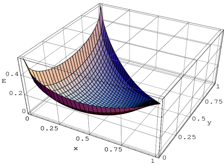
Figure 1: Entanglement vs. the composition of the pure state $|\psi(x,y)\rangle$.

A further property of the mixed state $\rho(x,y)$, which facilitates the computation of its entanglement, is a certain invariance, which we now describe. Consider the local unitary transformation a single qubit:

$$|0\rangle\rightarrow|0\rangle,$$ (6a)

$$|1\rangle\rightarrow g^{k}|1\rangle,$$ (6b)

where $g=\exp{(2\pi i/3)}$, i.e., a relative phase shift. This transformation, when applied simultaneously to all three qubits, is denoted by $U_{k}$. It is straightforward to see that $\rho(x,y)$ is invariant under the mapping

$$P:\rho\rightarrow\frac{1}{3}\sum_{k=1}^{3}U_{k}\,\rho\,U_{k}^{\dagger}\,.$$ (7)

Thus, we can apply Vollbrecht-Werner technique VollbrechtWerner01 ; WeiGoldbart02 to the compution of the entanglement of $\rho(x,y)$.

The first step of this task is to find the general form of the pure states that, under $P$, are projected to $\rho(x,y)$. This is readily seen to be

$$\sqrt{x}\,e^{i\phi_{1}}|GHZ\rangle+\sqrt{y}\,e^{i\phi_{2}}|W\rangle+\sqrt{1-x-y}\,e^{i\phi_{3}}|\widetilde{W}\rangle.$$ (8)

Of these, the least entangled state for given $(x,y)$ has all coefficients non-negative (up to a global phase), i.e.,

$$|\psi(x,y)\rangle\equiv\sqrt{x}|GHZ\rangle+\sqrt{y}|W\rangle+\sqrt{1-x-y}|\widetilde{W}\rangle.$$ (9)

The entanglement eigenvalue of $|\psi(x,y)\rangle$ can then be readily calculated (see Ref. WeiGoldbart02 for the strategy), and one obtains

$$\Lambda(x,y)=\frac{1}{(1\!+\!t^{2})^{\frac{3}{2}}}\Big{(}\sqrt{\frac{x}{2}}(1+t^{3})+\sqrt{3y}\,t+\sqrt{3(1\!-\!x\!-\!y)}\,t^{2}\Big{)},$$ (10)

where $t$ is the (unique) non-negative real root of the following third-order polynomial equation:

$$3\sqrt{\frac{x}{2}}(-t+t^{2})+\sqrt{3y}(-2t^{2}+1)$$

$$\qquad\qquad\quad+\sqrt{3(1-x-y)}(-t^{3}+2t)=0.$$ (11)

Hence, the entanglement function for $|\psi(x,y)\rangle$, i.e., $E_{\psi}(x,y)\equiv 1-\Lambda(x,y)^{2}$, is determined (up to root-finding).

Figure 2: Entanglement of the pure state $|\psi(x=0,y)\rangle=\sqrt{y}\,|{\rm W}\rangle+\sqrt{1-y}\,|\widetilde{\rm W}\rangle$ vs. $y$. This shows the entanglement along the $y$ axis.

Figure 3: Entanglement of the pure state $|\psi(x,y=1-x)\rangle=\sqrt{x}\,|GHZ\rangle+\sqrt{1-x}\,|W\rangle$ vs. $x$. This shows the entanglement along the diagonal boundary $x+y=1$. Note the absence of convexity near $x=1$; this region is repeated in the inset.

Recall that our aim is to determine the entanglement of the mixed state $\rho(x,y)$. As we now know the entanglement of the corresponding pure state $|\psi(x,y)\rangle$, we may accomplish our aim by invoking a result due to Vollbrecht and Werner VollbrechtWerner01 , which immediately gives the entanglement of $\rho(x,y)$ in terms of that of $|\psi(x,y)\rangle$, via the convex hull construction: $E_{\rho}(x,y)=(coE_{\psi})(x,y)$. Said in words, the entanglement surface $z=E_{\rho}(x,y)$ is the convex surface constructed from the surface $z=E_{\psi}(x,y)$.

The idea underlying the use of the convex hull this. Due to its linearity in $x$ and $y$, the state $\rho$ of Eq. (4) can [except when $(x,y)$ lies on the boundary] be decomposed into two parts: $\rho(x,y)=p\,\rho(x_{1},y_{1})+(1-p)\rho(x_{2},y_{2})$ with the weight $p$ and end-points $(x_{1},y_{1})$ and $(x_{2},y_{2})$ related by $p\,x_{1}+(1-p)x_{2}=x$ and $p\,y_{1}+(1-p)y_{2}=y$ . Now, if it should happen that $pE_{\psi}(x_{1},y_{1})+(1-p)E_{\psi}(x_{2},y_{2})<E_{\psi}(x,y)$ then the entanglement averaged over the end-points gives a value lower than that at the interior point $(x,y)$; this conforms with the convex-hull construction.

It should be pointed out that the convex hull should be taken with respect to parameters on which the density matrix depends linearly, as $x$ and $y$ do in the example of $\rho(x,y)$. Furthermore, in order to obtain the convex hull of a function, one needs to know the global structure of the function; in the present case, $E_{\psi}(x,y)$. We note that numerical algorithms have been developed for constructing convex hulls QHull .

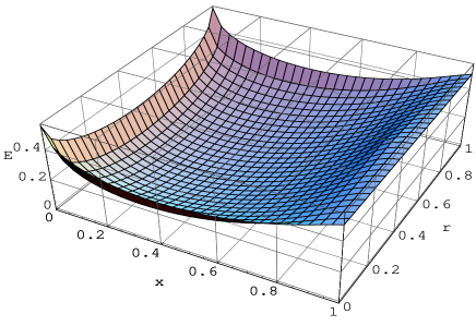
Figure 4: Entanglement of the pure state $|\psi\big{(}x,(1-x)r\big{)}\rangle=\sqrt{x}\,|GHZ\rangle+\sqrt{(1-x)r}\,|W\rangle+\sqrt{(1-x)(1-r)}|\widetilde{W}\rangle$ vs. $x$ and $r$. Note the symmetry of the surface with respect with $r=1/2$.

Figure 5: Entanglement of the pure states $|\psi\big{(}x,(1-x)r\big{)}\rangle=\sqrt{x}\,|GHZ\rangle+\sqrt{(1-x)r}\,|W\rangle+\sqrt{(1-x)(1-r)}|\widetilde{W}\rangle$ vs. $r$ for various values of $x$ (from the bottom: 0.8, 0.85, 0.9, 0.92, 0.94, 0.96, 0.98, 1). This reveals the nonconvexity in $r$ for intermediate values of $x$.

Figure 6: Entanglement of the pure states $|\psi\big{(}x,(1-x)r\big{)}\rangle=\sqrt{x}\,|GHZ\rangle+\sqrt{(1-x)r}\,|W\rangle+\sqrt{(1-x)(1-r)}|\widetilde{W}\rangle$ vs. $x$ for various values of $r$ (from the top: 0, 0.1, 0.2, 0.3, 0.5). This reveals the nonconvexity in $x$ in the (approximate) interval $[0.85,1]$.

As we have discussed, our route to establishing the entanglement of $\rho(x,y)$ invloves the analysis of the entanglement of $|\psi(x,y)\rangle$, which we show in Fig. 1. Although it is not obvious, the corresponding surface fails to be convex near to the point $(x,y)=(1,0)$, and therefore, in this region, we must suitably convexify in order to obtain the entanglement of $\rho(x,y)$. To illustrate the properties of the entanglement of $|\psi(x,y)\rangle$ we show, in Fig. 2, the entanglement of $|\psi(x,y)\rangle$ along the line $x=0$; evidently this is convex. By contrast, along the line $x+y=1$, there is a region in which the entanglement is not convex, as Fig. 3 shows. The nonconvexity of the entanglement of $|\psi(x,y)\rangle$ complicates the calculation of the entanglement of $\rho(x,y)$, as it necessitates a procedure for constructing the convex hull in the (as it happens, small) nonconvex region. Elsewhere in the $xy$ plane the entanglement of $\rho(x,y)$ is given directly by the entanglement of $|\psi(x,y)\rangle$.

Figure 7: Entanglement of the mixed state ${\rho(x,y)}$.

At worst, convexification would have to be undertaken numerically. However, in the present setting it turns out one can determine the convex surface essentially analytically, by performing the necessary surgery on surface $z=E_{\psi}(x,y)$. To do this, we make use of the fact that if we parametrize $y$ via $(1-x)r$, i.e., we consider

$${\rho\big{(}x,(1-x)r\big{)}} = x\,|GHZ\rangle\langle GHZ|+(1-x)r\,|W\rangle\langle W|$$ (12)

$$+(1-x)(1-r)|\widetilde{W}\rangle\langle\widetilde{W}|,$$

where $0\leq r\leq 1$ [and similarly for $|\psi(x,y)\rangle$] then, as a function of $(x,r)$, the entanglement will be symmetric with respect to $r=1/2$, as Fig. 4 makes evident. With this parametrization, the nonconvex region of the entanglement of $|\psi\rangle$ can more clearly be identified.

To convexify this surface we adopt the following convenient strategy. First, we reparametrize the coordinates, exchanging $y$ by $(1-x)r$. Now, owing to the linearity, in $r$ at fixed $x$ and vice versa, of the coefficients $x$, $(1-x)r$ and $(1-x)(1-r)$ in Eq. (12), it is certainly necessary for the entanglement of $\rho$ to be a convex function of $r$ at fixed $x$ and vice versa. Convexity is, however, not necessary in other directions in the $xr$ plane, owing to the nonlinearity of the the coefficients under simultaneous variations of $x$ and $r$. Put more simply: convexity is not necessary throughout the $(x,r)$ plane because straight lines in the $(x,r)$ plane do not correspond to straight lines in the $(x,y)$ plane (except along lines parallel either to the $r$ or the $x$ axis). Thus, our strategy will be to convexify in a restricted sense: first along lines parallel to the $r$ axis and then along lines parallel to the $x$ axis. Having done this, we shall check to see that no further convexification is necessary.

For each $x$, we convexify the curve $z=E_{\psi}\big{(}x,(1-x)r\big{)}$ as a function of $r$, and then generate a new surface by allowing $x$ to vary. More specifically, the nonconvexity in this direction has the form of a symmetric pair of minima located on either side of a cusp, as shown in Fig. 5. Thus, to correct for it, we simply locate the minima and connect them by a straight line.

What remains is to consider the issue of convexity along the $x$ (i.e., at fixed $r$) direction for the surface just constructed. In this direction, nonconvexity occurs when $x$ is, roughly speaking, greater than $0.8$, as Fig. 6 suggests. In contrast with the case of nonconvexity at fixed $r$, this nonconvexity is due to an inflection point at which the second derivative vanishes. To correct for it, we locate the point $x=x_{0}$ such that the tangent at $x=x_{0}$ is equal to that of the line between the point on the curve at $x_{0}$ and the end-point at $x=1$, and connect them with a straight line. This furnishes us with a surface convexified with respect to $x$ (at fixed $r$) and vice versa.

Armed with this surface, we return to the $(x,y)$ parametrization, and ask whether or not it is fully convex (i.e., convex along straight lines connecting any pair of points). Said equivalently, we ask whether or not any further convexification is required. Although we have not proven it, on the basis of extensive numerical exploration we are confident that the resulting surface is, indeed, convex. The resulting convex entanglement surface for $\rho(x,y)$ is shown in Fig. 7. Figure 8 exemplifies this convexity along the line $2y+x=1$. We have observed that for the case at hand it is adequate to correct for nonconvexity only in the $x$ direction at fixed $r$.

Figure 8: Entanglement of the mixed state ${\rho\big{(}x,y=(1-x)/2\big{)}}=x\,|GHZ\rangle\langle GHZ|+\frac{1-x}{2}\big{(}|W\rangle\langle W|+|\widetilde{W}\rangle\langle\widetilde{W}|\big{)}$ vs. $x$. Inset: enlargement of the region $x\in[0.2,0.3]$. This contains the only point, $(x,y)=(1/4,3/8)$, at which $E_{\rho}(x,y)$ vanishes.

Negativity: This measure of entanglement is defined as twice the absolute value of the sum of the negative eigenvalues of the partial transpose of the density matrix ZyczkowskiWerner ; WeiNemotoGoldbartKwiatMunroVerstraete03 . In the present setting, viz., the family $\rho(x,y)$ of three-qubit states, the partial transpose may equivalently be taken with respect to any one of the three parties, owing to the invariance of $\rho(x,y)$ under all permutations of the parties. Transposing with respect to the third party, one has

$$N(\rho)\equiv-2\sum_{\lambda_{i}<0}\lambda_{i},$$ (13)

where the $\lambda$’s are the eigenvalues of the matrix $\rho^{T_{3}}$,

It is straightforward to calculate the negativity for $\rho(x,y)$; the results are shown in Fig. 9. It is interesting to note that, for all allowable ranges of $(x,y)$, the state $\rho(x,y)$ has nonzero negativity, except at $(x,y)=(1/4,3/8)$, at which the calculation of the GME shows that the density matrix is indeed separable. The fact that the only positve-partial-transpose (PPT) state is separable is the statement that there are no entangled PPT states (i.e., no PPT bound entangled states) within this family of three-qubit mixed states. The negativity surface, Fig. 9, is qualitatively—but not quantitatively—the same as that of GME. By inspecting the negativity and GME surfaces one can see that they present ordering difficulties. We mean by this that one can find pairs of states $\rho(x_{1},y_{1})$ and $\rho(x_{2},y_{2})$ that respectively have negativities $N_{1}$ and $N_{2}$ and GMEs $E_{1}$ and $E_{2}$ such that, say, $N_{1}<N_{2}$ but $E_{1}>E_{2}$. Said equivalently, the negativity and the GME do not necessarily agree on which of a pair of states is the more entangled. For two qubit settings, such ordering difficulties do not show up for pure states but can for mixed states Ordering ; WeiNemotoGoldbartKwiatMunroVerstraete03 . On the other hand, such difficulties already show up for pure states, as the following example shows: $N(GHZ)=1>N(W)=2\sqrt{2}/3$ whereas for the GME the order is reversed. We note that for the relative entropy of entanglement $E_{R}$, one has $E_{R}(GHZ)=\log 2<E_{R}(W)=\log(9/4)$PlenioVedral01 .

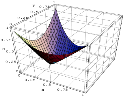
Figure 9: Negativity of the mixed state ${\rho(x,y)}$.

Concluding remarks: By making use of the geometric measure of entanglement we have addressed the entanglement of a rather general family of three-qubit mixed states analytically (up to root-finding). This family consists of arbitrary mixtures of GHZ, W, and inverted-W states. To the best of our knowledge, corresponding results have not, to date, been obtained for other measures of entanglement, such as entanglement of formation and relative entropy of entanglement. We have obtained corresponding results for the negativity measure of entanglement, and have compared them with those for the geometric measure of entanglement. Among other things, we have found that there are no PPT bound entangled states within this general family.

We are unaware of any explicit generalization of entanglement of formation to multipartite mixed states. However, if such a generalization should emerge, and if it should be based on the convex hull construction (as it is in the bipartite case), then one may be able to calculate the entanglement of formation for the family of mixed states considered in the present Paper. It would, then, be interesting to know whether or not the similarities between entanglement of formation and the geometric measure of entanglement found at the level of certain bipartite mixed states WeiGoldbart02 continue to hold beyond the bipartite world.

Acknowledgments: We thank J. Altepeter, H. Edelsbrunner, M. Ericsson, P. Kwiat, S. Mukhopadhyay, F. Verstraete and especially W. J. Munro for discussions. This work was supported by NSF EIA01-21568. and DOE DEFG02-91ER45439. TCW acknowledges a Mavis Memorial Fund Scholarship.

References

- (1) T. C. Wei and P. M. Goldbart, quant-ph/0212030.
- (2) A. Shimony, Ann. NY. Acad. Sci. 755, 675 (1995).
- (3) H. Barnum and N. Linden, J. Phys. A: Math. Gen. 34, 6787 (2001); also in quant-ph/0103155.
- (4) See, e.g., M. Nielsen and I. Chuang, Quantum Computation and Quantum Information (Cambridge University Press, 2000).
- (5) For a review, see M. Horodecki, Quant. Info. Comp. 1, 3 (2001), and references therein.
- (6) T. C. Wei and P. M. Goldbart, quant-ph/0303079.
- (7) W. K. Wootters, Phys. Rev. Lett. 80, 2245 (1998).
- (8) K. G. H. Vollbrecht and R. F. Werner, Phys. Rev. A 64, 062307 (2001).
- (9) See e.g., C. B. Barber, D. P. Dobkin, and H. T. Huhdanpaa, ACM Trans. on Mathematical Software 22, 469 (1996).
- (10) K. Życzkowski et al., Phys. Rev. A 58, 883 (1998); G. Vidal and R. F. Werner, Phys. Rev. A 65, 032314 (2002).
- (11) T. C. Wei, K. Nemoto, P. M. Goldbart, P. G. Kwiat, W. J. Munro, and F. Verstraete, Phys. Rev. A 67, 022110 (2003); also in quant-ph/0208138.
- (12) This ordering difficulty has been discussed in the settings of two qubits in many places, e.g., J. Eisert and M. B. Plenio, J. Mod. Opt. 46, 145 (1999); K. Życzkowski, Phys. Rev. A 60, 3496 (1999); S. Virmani and M. B. Plenio, Phys. Lett. A 268, 31 (2000); F. Verstraete et al., J. Phys. A 34, 10327 (2001), as well as in Ref. WeiNemotoGoldbartKwiatMunroVerstraete03 .
- (13) M. B. Plenio and V. Vedral, J. Phys. A 34, 6997 (2001).