Bounds for Entanglement of formation of two mode squeezed thermal States

Abstract

The upper and lower bounds of entanglement of formation are given for two mode squeezed thermal state. The bounds are compared with other entanglement measure or bounds. The entanglement distillation and the relative entropy of entanglement of infinitive squeezed state are obtained at the postulation of hashing inequality.

Keywords: bound of entanglement measure, two mode squeezed thermal state,

PACS: 03.67.-a,03.65.Bz

Quantum entanglement plays an essential role in all branches of the emerging field of quantum information[1]. Recently a great deal of attention has been devoted to the quantum information processing with canonical continuous variables and various protocols for quantum communication and computation are developed based on continuous variables [2] [3] [4]. With continuous variable optical system these protocols can be implemented. The efficiency of entanglement manipulation protocols critically depends on the quality of the entanglement that one can generate. For practical purpose [5] one needs to determine the entanglement degradation in transmission of two mode squeezed vacuum state light through absorbing fibers. It is therefore essential to be able to quantify the amount of entanglement in systems with continuous variables.

Of all the continuous variable quantum states, quantum Gaussian states are of great practical importance, since these comprise essentially all the experimentally realizable continuous variable states, theoretically they might also be simple enough to be analytically tractable for the problems involved. Gaussian state is completely specified by its mean $\eta$ and its correlation matrix $\alpha$, where the mean can be dropped by local unitary operation so that is irrelevant for entanglement problems. The density operator of Gaussian state can be characterized [6] by its quantum characteristic function $\chi\left(z\right)=\exp[i\eta^{T}z-\frac{1}{2}z^{T}\alpha z]$ , and any Gaussian state of two modes can be transformed into what we called the standard form, using local unitary operation only [7] [8]. The corresponding characteristic function has mean $\eta=0$ and the correlation matrix has the simple form

$$\alpha=\left[\begin{array}[c]{llll}b_{1},&0,&c_{1},&0\\ 0,&b_{1},&0,&c_{2}\\ c_{1},&0,&b_{2},&0\\ 0,&c_{2},&0,&b_{2}\end{array}\right],$$ (1)

A particular simple subset of two mode Gaussian states is the two mode squeezed thermal states (TMST), with $b_{1}=b_{2}=b,$ $c_{1}=-c_{2}=c$. The density operator of  TMST is $\rho_{ST}=S_{2}^{+}\left(r\right)\rho_{0}S_{2}\left(r\right),$ where $S_{2}\left(r\right)=\exp[-r(a_{1}^{+}a_{2}^{+}-a_{1}a_{2})]$ is the two mode squeezed operator with squeezing parameter $r\geq 0$, and $\rho_{0}$ is the product of two thermal states A and B whose average photon numbers are $N_{A}=N_{B}=N$. The relationship between the two expressions of TMST is $b=(N+1/2)\cosh 2r,$ $c=(N+1/2)\sinh 2r$. One can use the unit scale parameters $\lambda=\tanh r$ and $v=N/(N+1)$, then the inseparability criterion has a very simple form of $\lambda>v$[7] [8].

Even for the two parameter TMST, however, until now the amount of the entanglement in several main measures remains an open question. In this paper, I will study the upper and lower bounds for the entanglement of formation of TMST. First I will establish the lower bound of entanglement of formation, then the upper bound, then compare them with other entanglement bounds and measure, at last draw the conclusions.

Now let us consider the lower bound of entanglement of formation. It was proved that entanglement of formation is nonincreasing under local operation and classical communication [9]. This presents us a nature way to obtain the lower bound of the entanglement of formation of a mixed state. By performing a special kind of local operation and (or) classical communication to the state, converting it to a state whose entanglement of formation is well known, the entanglement of formation of the resultant state will provide a lower bound to that of the original state.

For TMST, the simplest way of conversion is to map it on a two-qubit system by means of local operation. One of the operation for such purpose is with the Hermitian spin one-half operators[10] $S_{j}^{\mu},$ $\mu=A,B$ for A, B parts respectively, $S_{1}^{\mu}+iS_{2}^{\mu}=2\sum_{m=0}^{\infty}\left|2m\right\rangle_{\mu\mu}\left\langle 2m+1\right|,S_{3}^{\mu}=\sum_{m=0}^{\infty}\left(-1\right)^{m}\left|m\right\rangle_{\mu\mu}\left\langle m\right|,$which satisfy the Pauli matrix algebra: $\left[S_{i}^{\mu},S_{j}^{\nu}\right]=2i\varepsilon_{ijk}\delta_{\mu\nu}S_{k}^{\mu}$.

Let us denote the mapped state with $\rho^{\prime}$ and assign the following qubit density matrix $\rho^{\prime}_{A}$ to the original reduced density matrix $\rho_{A}$, $\rho^{\prime}_{A}=\frac{1}{2}\left(I_{A}+\mathbf{S}^{A}\cdot\mathbf{\sigma}\right),$where $\mathbf{S}^{A}\mathbf{\cdot\sigma}=\sum_{i=1}^{3}Tr\left(\rho_{A}S_{i}^{A}\right)\sigma_{i}$, $\ \sigma_{i}$ are Pauli matrices and $I_{A}$ is the identity operator on the Hilbert space of qubit A.

The map of bipartite density matrix is[10]

$$\rho^{\prime}=\frac{1}{4}\left(I_{A}\otimes I_{B}+\mathbf{S}^{A}\cdot\mathbf{\sigma}\otimes I_{B}+I_{A}\otimes\mathbf{S}^{B}\cdot\mathbf{\sigma+}\sum_{i,j}t_{ij}\sigma_{i}\otimes\sigma_{j}\right)$$

, with $t_{ij}=Tr\left(\rho S_{i}^{A}S_{j}^{B}\right)$ .

For TMST density matrix $\rho_{ST}$, its reduced state $\rho_{A}$ $=Tr_{B}\rho_{ST}$ turns out to be a one mode thermal state of the form $\left(1-v^{\prime}\right)\sum_{m=0}^{\infty}v^{\prime m}\left|m\right\rangle\left\langle m\right|$ with $v^{\prime}=\frac{v+\lambda^{2}}{1+v\lambda^{2}}$ . It is clear that $Tr\left(\rho_{A}S_{1,2}^{A}\right)=0$, and a direct calculation shows that $Tr\left(\rho_{A}S_{3}^{A}\right)=\frac{1-v^{\prime}}{1+v^{\prime}}$. Meanwhile the two mode squeezing operator $S_{2}\left(r\right)$ will generate or annihilate the same number of bosons in mode A and mode B, it will not change the difference of the occupation numbers of the two modes, one readily gets $t_{ij}=0$, for $i\neq j$. As for the diagonal elements $t_{ii}$, from the definition of $t_{ij}$ , it follows that $t_{11}=-t_{22}=2Tr\sum_{m,n=0}^{\infty}\rho_{ST}\left|2m,2n\right\rangle\left\langle 2m+1,2n+1\right|.$Making use of the coherent state representation of $\rho_{ST}$ ,after some algebra, one obtains $t_{33}=\left(\frac{1-v}{1+v}\right)^{2}$ and

$$t_{11}=2C_{0}\sum_{m,n=0}^{\infty}\sum_{l=0}^{2\min\left(m,n\right)}\sqrt{\frac{2n+1}{2m+1}}\left(\begin{array}[]{c}2m+1\\ l+1\end{array}\right)\left(\begin{array}[]{c}2n\\ l\end{array}\right)\tau^{2l+1}\omega^{2m+2n-2l},$$ (2)

with $C_{0}=\frac{\left(1-v\right)^{2}\left(1-\lambda^{2}\right)}{1-v^{2}\lambda^{2}}$, $\tau=\frac{\lambda\left(1-v^{2}\right)}{1-v^{2}\lambda^{2}}$ , $\omega=\frac{v\left(1-\lambda^{2}\right)}{1-v^{2}\lambda^{2}}$.

The qubits map of TMST is

$$\rho^{\prime}=\left[\begin{array}[c]{llll}\frac{1+v^{2}\lambda^{2}}{\left(1+v\right)^{2}\left(1+\lambda^{2}\right)},&0,&0,&\frac{t_{11}}{2}\\ 0,&\frac{v}{\left(1+v\right)^{2}},&0,&0\\ 0,&0,&\frac{v}{\left(1+v\right)^{2}},&0\\ \frac{t_{11}}{2},&0,&0,&\frac{v^{2}+\lambda^{2}}{\left(1+v\right)^{2}\left(1+\lambda^{2}\right)}\end{array}\right]$$ (3)

The concurrence [11] of $\rho^{\prime}$ will be $C=\max\{0,t_{11}-2v/\left(1+v\right)^{2}\}$. Denote $x=\frac{1}{2}\left(1+\sqrt{1-C^{2}}\right)$, the entanglement of formation of $\rho^{\prime}$ reads

$$E\left(\rho^{\prime}\right)=h\left(x\right)=-x\log x-(1-x)\log(1-x).$$ (4)

Throughout this paper the base of $\log$ is $2$. One then obtains the lower bound of entanglement of formation : $E_{lf}\left(\rho_{ST}\right)=E\left(\rho^{\prime}\right)$.

We now turn to the upper bound for entanglement of formation of quantum Gaussian state and specifically TMST. The entanglement of formation is defined as follows[9]. Given a density matrix $\rho$ of bipartite quantum system, consider all possible pure state decompositions of $\rho$, that is, all ensembles of states $\left|\psi_{i}\right\rangle$ with probabilities $p_{i}$, such that $\rho=\sum_{i}p_{i}\left|\psi_{i}\right\rangle\left\langle\psi_{i}\right|$. For each pure state $\left|\psi\right\rangle$, the entanglement $E\left(\psi\right)$ is defined as the entropy of the reduced state of $\left|\psi\right\rangle$. The entanglement of formation of the mixed state $\rho$ is then defined as the average entanglement of the pure states of the decomposition, minimized over all decompositions of $\rho:$ $E\left(\rho\right)=\min\sum_{i}p_{i}E\left(\psi_{i}\right)$.

From the definition, it is known that any ensemble as a decomposition of $\rho$ has an average entanglement no less than the entanglement of formation of $\rho$, and so that is a candidate in providing an upper bound for the entanglement of formation of $\rho$ . The aim of us is to construct a series of decompositions, and within the series find out the decomposition of minimum average entanglement. Because the series is just a subset of the set of all possible decompositions, the minimum within the series is a local minimum. It provides a relatively tight upper bound for global minimum, the entanglement of formation of $\rho$.

Among all the decompositions, Gaussian state decomposition is mathematically easy to deal with. Rather than decompose a Gaussian state to its pure Gaussian state ensemble, let us generate mixed Gaussian state from a pure Gaussian seed. In the viewpoint of quantum channel, the way of generating mixed Gaussian state from a pure Gaussian state is just the way of transmitting the pure Gaussian state through quantum Gaussian channel [12]. So that the problem of how to generate mixed Gaussian state is physical, at least in principle. Suppose a pure Gaussian state is given with correlation matrix $\alpha_{s}$ and zero mean. Applying local unitary displacement operation on it yields another pure Gaussian state, with the same correlation matrix but a nonzero mean value or displacement $\eta$. The two states have the same amount of entanglement because local unitary operation does not change entanglement of pure state share by two parts A and B. If the displacement $\eta$ has a Gaussian probability distribution, then the mixture of all these Gaussian states will be a Gaussian state[6]. Let $P$ be a Gaussian probability distribution with zero mean (for convenience) and covariance matrix $M$ for variables $\left(\eta_{A}^{q},\eta_{A}^{p},\eta_{B}^{q},\eta_{B}^{p}\right)$ =$\eta^{T}$. The quantum characteristic function of the mixed state $\rho_{P}$ is

$$\int\exp(i\eta^{T}z-\frac{1}{2}z^{T}\alpha_{s}z)P\left(d\eta\right)=\exp[-\frac{1}{2}z^{T}\left(M+\alpha_{s}\right)z].$$ (5)

The correlation matrix of $\rho_{P}$ is $\alpha_{P}=M+\alpha_{s}$. Normalizable of probability measure requires that $M$ should be positive semi-definite, $M=0$ is included to correspond to $\delta$ function type of probability distribution. So that arbitrary Gaussian mixed state $\rho_{P}$ can be decomposed into an ensemble of pure Gaussian states as far as the difference of the correlation matrices is positive semi-definite. That is

$$M=\alpha_{P}-\alpha_{s}\geq 0.$$ (6)

So if the separable pure Gaussian state correlation matrix $\alpha_{s}$ is found under the restriction of Eq. (6), state $\rho_{P}$ should be separable. If it is impossible to find such an $\alpha_{s}$, then one has to turn to find an entangled pure Gaussian state correlation matrix $\alpha_{s}$ to fulfill Eq.(6). The minimum of the entanglement of those pure entangled Gaussian states will give out the upper bound of entanglement of formation of state $\rho_{P}$.

Consider the entangled TMST $\rho_{ST}$ with $\lambda>v$. Let

$$\alpha_{s}=\frac{1}{2}\left[\begin{array}[c]{llll}\cosh 2x,&0,&\sinh 2x,&0\\ 0,&\cosh 2x,&0,&-\sinh 2x\\ \sinh 2x,&0,&\cosh 2x,&0\\ 0&-\sinh 2x,&0,&\cosh 2x\end{array}\right],$$ (7)

be exactly the squeezed vacuum state with squeezing parameter $x$. $M\geq 0$ requires that $b-\frac{1}{2}\cosh 2x\geq 0,(b-\frac{1}{2}\cosh 2x)^{2}-(c-\frac{1}{2}\sinh 2x)^{2}\geq 0.$This can be written as $\cosh 2\left(r-x\right)\leq\frac{1+v^{2}}{1-v^{2}}.$Denote $v=\tanh w$, one gets $r-x\leq w,$ or $x\geq r-w$. The minimum is $x_{0}=r-w$. Let $y=\sinh^{2}x_{0},$ in explicit form of $\lambda,v$, one has $y=\frac{\left(\lambda-v\right)^{2}}{\left(1-\lambda^{2}\right)\left(1-v^{2}\right)}$. The upper bound of entanglement of formation then will be

$$E_{uf}\left(\rho_{ST}\right)=g\left(y\right)=\left(y+1\right)\log\left(y+1\right)-y\log y$$ (8)

Let us compare the entanglement bounds obtained above with other bounds and entanglement measure. First of them is the upper bound of relative entropy of entanglement. The entanglement measure is defined by the minimization of the distance of the entangled Gaussian state to the set of separable states measured by the relative entropy, its bound was obtained by restricting the minimization set to that of separable Gaussian states[5]. We can further restrict  it to the set of separable TMST $\widetilde{\rho}_{ST}=S_{2}\left(\widetilde{r}\right)\rho_{0}\left(\widetilde{v}\right)S_{2}^{+}\left(\widetilde{r}\right)$, with $\widetilde{\lambda}=\tanh\widetilde{r}\leq\widetilde{v}$. Then the minimization can be carried out. The upper bound will be

$$E_{ur}\left(\rho_{ST}\right)=-2g\left(N\right)-2\log\left(1-\widetilde{v}^{\ast}\right)-[\frac{1+v}{1-v}\cosh\left(r-\widetilde{w}^{\ast}\right)-1]\log\widetilde{v}^{\ast}.$$ (9)

The minimum reaches at $\widetilde{\lambda}=\widetilde{v}=\widetilde{v}^{\ast}=\tanh\widetilde{w}^{\ast}$ for some $\widetilde{v}^{\ast}$.

The second one we should compare with is entanglement measure of logarithmic negativity [13], for TMST, it reads

$$E_{LN}(\rho_{ST})=\log[(1+\lambda)(1-v)]-\log[(1-\lambda)(1+v)].$$ (10)

The last one used in comparing is coherent information. The coherent information of bipartite state $\sigma$ with reductions $\sigma_{A}$ and $\sigma_{B}$ is defined as [14]$I^{\mu}\left(\sigma\right)=S\left(\sigma_{\mu}\right)-S\left(\sigma\right),$for $S\left(\sigma_{\mu}\right)-S\left(\sigma\right)\geq 0$ and $I^{\mu}\left(\sigma\right)=0$ otherwise, where $S$ denotes the von Neumann entropy. And if for any bipartite state the one-way distillable entanglement is no less than coherent information which is called hashing inequality, then one obtains Shannon-like formulas for the capacities [15]. The hypothetical hashing inequality reads

$$D_{\rightarrow}\left(\sigma\right)\geq I^{B}\left(\sigma\right)$$ (11)

where $D_{\rightarrow}\left(\sigma\right)$ is forward classical communication aided distillable entanglement of the state. I do not mean to prove this inequality, but rather to check if it is violated for some cases in continuous variable system. It is known that two way distillation of entanglement is no less than that of one way[9], and entanglement of formation is no less than relative entropy of entanglement[16], the later is no less than distillation of entanglement[17]. In short one has $E_{f}\left(\sigma\right)\geq E_{r}\left(\sigma\right)\geq D_{\leftrightarrow}\left(\sigma\right)\geq D_{\rightarrow}\left(\sigma\right)$. Combining with hashing inequality one then obtains

$$E_{uf}\left(\sigma\right)\geq E_{f}\left(\sigma\right)\geq I^{B}\left(\sigma\right),\quad E_{ur}\left(\sigma\right)\geq E_{r}\left(\sigma\right)\geq I^{B}\left(\sigma\right).$$ (12)

For TMST $\rho_{ST}$,  the entropy of its reduced state is $g\left(N^{\prime}\right)$, with $N^{\prime}=\frac{v^{\prime}}{1-v^{\prime}}=\frac{v+\lambda^{2}}{\left(1-v\right)\left(1-\lambda^{2}\right)}$. The coherent information is

$$I^{B}\left(\rho_{ST}\right)=\max\{g\left(N^{\prime}\right)-2g\left(N\right),0\}$$ (13)

By comparison of all bounds and measure of TMST I find that: (1) the upper bound of entanglement of formation and of relative entropy of entanglement are no less than coherent information, so it can be anticipated that hashing inequality is also true for TMST or more generally for bipartite Gaussian state; (2) As the squeezing parameter tends towards zero, the lower and upper bounds of entanglement of formation tend to coincide with each other. (3) As the squeezing parameter tends towards infinitive, the upper bound of relative entropy of entanglement tends to coincide with the coherent information, so if the hashing inequality is right, the relative entropy of entanglement, the distillation entanglement and coherent information are all equal for infinitive squeezing state. (4) The entanglement measure of logarithmic negativity is at the topmost of all the bounds.

The main points of this paper are as follow: (1) The lower bound of entanglement of formation of TMST is drawn from the fact that local operation can only decreases if not preserves the entanglement, at lower squeezing side, it almost coincides with the upper bound. This result leads to the possible determination of the entanglement of formation at lower squeezing level. (2)As for the upper bound of entanglement of formation of quantum Gaussian state, an inequality is derived, for the case of TMST, an analytical expression is given out. (3)By carrying out the minimization of the upper bound of relative entropy of entanglement[5] for TMST I determine the entanglement distillation and the relative entropy of entanglement of TMST with infinitive squeezing at the postulation of hashing inequality.

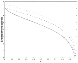
Figure 1: Comparison of bounds and measure at $\lambda\rightarrow 1$ side. $\lambda=0.99,$ dashed line for $E_{uf}$, dashdot for $E_{ur}$, solid for $I^{B}$, dotted for $E_{LN}$

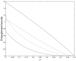
Figure 2: Comparison of bounds and measure at $\lambda=0.5,$ dashed line for $E_{uf}$, dashdot for $E_{ur}$, the lower solid for $E_{lf}$, dotted for $I^{B}$. the topmost solid for $E_{LN}$.

Figure 3: Comparison of bounds at $\lambda\rightarrow 0$ side. $\lambda=0.01,$ dashed line for $E_{uf}$, dashdot for $E_{ur}$, solid for $E_{lf}$, dotted for$I^{B}$. Entanglement measure $E_{LN}$ is omitted for significantly greater than the bounds.

References

• [1] C. H. Bennett, Phys. Today 48, No 10, 24 (1995); D. P. DiVincenzo, Science 270, 255 (1995).
• [2] S. L. Braunstein and H. J. Kimble, Phys. Rev. Lett. 80, 869 (1998); S. L. Braunstein, Nature. 394, 47 (1998).
• [3] S. Lloyd and S. L. Braunstein, Phys. Rev. Lett. 82, 1784 (1999).
• [4] D. Gottesman, A. Kitaev and J. Preskill, Phys. Rev. A 64, 012310 (2001).
• [5] S. Scheel and D.-G. Welsch, arXiv: quant-ph/0103167.
• [6] A. S. Holevo, M. Sohma and O. Hirota, Phys. Rev. A 59, 1820 (1999).
• [7] L. M. Duan, G. Giedke, J. I. Cirac and P. Zoller, Phys. Rev. Lett. 84, 2722 (2000).
• [8] R. Simon, Phys. Rev. Lett. 84, 2726 (2000)
• [9] C. H. Bennett, D. P. DiVincenzo, J. A. Smolin and W. K. Wootters, Phys. Rev. A 54, 3824 (1996).
• [10] L. MiΕ‘ta, Jr. R. Filip and J. FiurΓ‘Ε‘ek, Phys. Rev. A 65, 062315 (2002).
• [11] W. K. Wootters, Phys. Rev. Lett. 80, 2245 (1998).
• [12] X.Y. Chen and P. L. Qiu, Chin. Phys. 10, Β 779 (2001)
• [13] G. Vidal and R. F. Werner, Phys. Rev. A 65, 032314 (2002).
• [14] B. Schumacher, Phys. Rev. A 54, 2614 (1996); B. Schumacher and M. A. Nielsen, Phys. Rev. A 54, 2629 (1996).
• [15] M. Horodecki, P.Horodecki and R.Horodecki, Phys. Rev. Lett. 85, 433 (2000).
• [16] V. Vedral and M. B. Plenio, Phys. Rev. A 57, 1619 (1998).
• [17] V. Vedral, Rev. Mod. phys. 74, 197 (2002).
Refer to caption