Directly Observing Momentum Transfer in Twin-Slit “Which-Way” Experiments

Abstract

Is the destruction of interference by a which-way measurement due to a random momentum transfer $\wp\gtrsim\hbar/s$, with $s$ the slit separation? The weak-valued probability distribution $P_{\rm wv}(\wp)$, which is directly observable, provides a subtle answer. $P_{\rm wv}(\wp)$ cannot have support on the interval $[-\hbar/s,\hbar/s]$. Nevertheless, its moments can be identically zero.

I Introduction

Making a position measurement to determine through which slit a particle has passed necessarily destroys the twin-slit interference pattern (see Fig. 1). This is the canonical example of Bohr’s complementarity principle BohrEinst ; WheZur83 . To defend this principle against Einstein’s recoiling slit gedankenexperiment, Bohr relied upon the recently (in 1927) derived Heisenberg uncertainty relation Hei27 to show that the position measurement would cause an “uncontrollable change in the momentum” $\wp\gtrsim\hbar/s$, where $s$ is the slit separation BohrEinst . This is just what is required to wash out the interference pattern, thereby enforcing complementarity. Bohr’s argument was famously reiterated by Feynman FeyLeiSan65 , for a measurement using Heisenberg’s light microscope Hei27 .

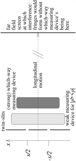
Figure 1: Diagram of a twin-slit which-way experiment. The initial state $|{\psi_{i}}\rangle$ is formed by the slits and propagates longitudinally towards the final screen. This is in the far field, so detecting the position of the particle there is equivalent to measuring its final momentum $p_{f}$. With the which-way measurement (WWM) device in place the distribution for $p_{f}$ is just the single-slit diffraction pattern. In its absence, a twin-slit interference pattern would form. Between the slits and the WWM device is a device which makes a weak measurement of $|{p_{i}}\rangle\langle{p_{i}}|$, as explained later in the text.

In 1991 Scully, Englert and Walther ScuEngWal91 proposed a new which-way (welcher Weg) scheme for which, they calculated, no momentum would be transferred to the particle. Thus, they concluded, the arguments of Bohr and Feynman were wrong in general, and that complementarity must be deeper than uncertainty. Storey, Tan, Collett and Walls (STCW) StoTanColWal94 disagreed, proving a theorem that if interference is destroyed then there is some transverse momentum transfer $\geq\hbar/s$. The debate QI94 ; Nature95 was partially resolved when it was pointed out WisHar95 that SEW and STCW were using different concepts of “momentum transfer”, and that their analyses were in fact complementary. Aspects of both are found in two further characterizations of momentum transfer that have since been proposed Wis97a ; Wis98a . However, these characterizations are not obtainable from experiments directly (i.e. in a way that would make sense to a classical physicist).

In this Letter I propose a new and attractive resolution: a way to directly observe a single probability distribution $P(\wp)$ for momentum transfer $\wp$ in a which-way measurement (WWM). My method shows that SEW were right, in that the variance of $P(\wp)$ is zero for their scheme, but that STCW were also right, in that $P(\wp)$ cannot have support on the interval $[-\hbar/s,\hbar/s]$. This is possible only because $P(\wp)$ must be measured as a weak valued AhaAlbVai88 probability distribution, and hence may take negative values.

The body of this Letter is organized as follows. First I introduce the general formalism of WWMs, and use this to explain the four characterizations of momentum transfer proposed in Refs. ScuEngWal91 ; StoTanColWal94 ; Wis97a ; Wis98a . I discuss these characterizations in terms of 6 key properties, showing that each lacks at least 2 properties. This motivates the introduction of the present approach, based on weak values, which has all properties except non-negativity of $P(\wp)$.

II Which-way measurements

Say the two slits in the Young’s interferometer are centred at $x=\pm s/2$. Note that it is necessary to restrict the discussion to an interferometer of this kind, where the initial superposition is in transverse position and the free evolution preserves the conjugate quantity (transverse momentum), so that the issue of loss of visibility related directly to transverse momentum transfer. Analogous issues may be identifiable for other sorts of interferometer, but that is beyond the scope of this Letter.

A generalized measurement of $x$ transforms the initial state produced by the twin slits, $|{\psi_{i}}\rangle$, into a final mixed state, $\rho_{f}$, according to StoTanColWal94 ; Wis97a

$$\rho_{f}=\hat{O}_{\xi}|{\psi_{i}}\rangle\langle{\psi_{i}}|\hat{O}_{\xi}^{\dagger}.$$ (1)

Here $\left\{{\xi}\right\}$ is the set of measurement results, which here is summed over, as I am using the Einstein summation convention. This gives the final state averaged over all possible results, because $\hat{O}_{\xi}|{\psi_{i}}\rangle$ represents the unnormalized state given the result $\xi$, and its modulus squared is the probability to obtain that result $\xi$.

Note that there are infinitely many sets of operators $\{\hat{O}_{\xi}\}$ which give the same average transformation (1) TanWal93 . These different sets can be obtained physically by using the same measurement interaction between the system and the apparatus, but from resolving this apparatus in different bases. For example, for many measurements there is a “quantum eraser” basis ScuDru82 complementary to the basis that gives the best which-way information. In these different bases, the states $\hat{O}_{\xi}|{\psi_{i}}\rangle$ conditioned on individual results may be completely different, but the average state $\rho_{f}$ is the same.

For Eq. (1) to describe a position measurement, it is necessary to restrict the operators $\hat{O}_{\xi}$ to be functions of the position operator $\hat{x}$. Then in the position representation one finds

$$\langle{x}|\hat{O}_{\xi}|{\psi_{i}}\rangle=O_{\xi}(x)\psi_{i}(x).$$ (2)

Thus the measurement is defined by the functions $\left\{{O_{\xi}(x)}\right\}$, which are constrained mathematically only by the completeness condition

$$\forall x\;O_{\xi}(x)O_{\xi}^{*}(x)=1$$ (3)

which ensures that $\rho_{f}$ is normalized. For narrow slits, [i.e. $|\psi(x)|^{2}\simeq\delta(2x+s)+\delta(2x-s)$], the visibility of the far field interference pattern can be shown Wis97a to be given by

$$V=\left|{O_{\xi}(-s/2)O_{\xi}^{*}(s/2)}\right|.$$ (4)

It is evident from Eq. (2) that if all of the $O_{\xi}(x)$ are flat in the region of the slits, then a single slit initial wavefunction $\psi_{i}(x)$ will emerge unchanged from the measurement region. In particular, its momentum distribution (the diffraction pattern) will be no wider than that with no measurement. This phenomenon is compatible with the complete loss of visibility (4), and indeed would occur for the micromaser experiment proposed by SEW. It is by this directly observable measure that SEW claimed there would be no momentum transfer.

In response, STCW proved that Eqs. (3) and (4) imply that for at least one $\xi$, the Fourier transform

$$\tilde{O}_{\xi}(p)=(2\pi\hbar)^{-1/2}\int\!dx\,O_{\xi}(x)e^{-ixp/\hbar}$$ (5)

does not have support on the interval $(-\hbar/s,\hbar/s)$ if $V=0$. The significance of this is that in the momentum representation Eq. (2) becomes

$$\langle{p}|\hat{O}_{\xi}|{\psi_{i}}\rangle=\int\!d\wp\,\tilde{O}_{\xi}(\wp)\tilde{\psi}_{i}(p-\wp).$$ (6)

This implies that $\tilde{O}_{\xi}(\wp)$ can be interpreted as a momentum transfer amplitude distribution. Moreover, from Eq. (6), if the initial state $|{\psi_{i}}\rangle$ were a $p=0$ momentum eigenstate then the final momentum distribution would be $\langle{p}|\rho_{f}|{p}\rangle=\tilde{O}_{\xi}(p)\tilde{O}_{\xi}^{*}(p)$. Thus the momentum transfer in the STCW theorem is also directly observable, as the creation of momentum components greater than or equal to $\hbar/s$.

For the Einstein recoiling slit BohrEinst and Feynman light microscope FeyLeiSan65 , it turns out that

$$\langle{p}|\rho_{f}|{p}\rangle=\int\!d\wp\,P_{\rm classical}(\wp)|\tilde{\psi}_{i}(p-\wp)|^{2}$$ (7)

where $P_{\rm classical}(\wp)$ is non-negative. For such schemes the $O_{\xi}(x)$ can be chosen as $\sqrt{N_{\xi}}\exp(-ik_{\xi}x)$, and $P_{\rm classical}(\wp)=\sum_{\xi}N_{\xi}\delta(\wp-\hbar k_{\xi})$. For these schemes, the final momentum distribution is broadened identically for all initial states, and the SEW and STCW characterizations of momentum transfer agree. However, for some schemes (most notably that of SEW) the functions $O_{\xi}(x)$ are necessarily not of this form, which is why more than one characterization of momentum transfer is possible in general. These facts were first pointed out by Wiseman and Harrison WisHar95 .

The essential problem is that if the momentum transfer (6) is not of classical form (7), then the transfer of momentum is not clearly defined for an initial twin-slit state, as it does not have definite momentum. The obvious solution is to use a quantum formalism in which a momentum is associated with the particle even when it is not in a momentum eigenstate. Two such formalisms have been investigated in the past.

In the Wigner function formalism Wis97a , the particle is described by a pseudo probability distribution on phase space $W(x,p)$ which gives the correct marginal distributions for $x$ and $p$. The transformation Eq. (1) becomes

$$W_{f}(p,x)=\int\!d\wp\,W_{i}(x,p-\wp)P_{\rm Wigner}(\wp;x).$$ (8)

Here $P_{\rm Wigner}(\wp;x)$ is defined in terms of $\left\{{O_{\xi}}\right\}$ and acts formally as an $x$-dependent momentum transfer probability distribution. Both the local momentum transfer at $x=\pm s/2$, and the nonlocal momentum transfer at $x=0$ (midway between the slits) are relevant to the final momentum distribution.

In the Bohmian formalism Wis98a , an individual particle has a definite position $x$ and momentum $p=m\dot{x}={\rm Re}[-i\hbar\psi^{\prime}(x)/\psi(x)]$. The probability distribution for $x$ is the usual $|\psi(x)|^{2}$, but that for $p$ equals $|\tilde{\psi}(p)|^{2}$ only in the far field Boh52 . By following the trajectories of individual particles one can calculate a time-dependent momentum transfer probability distribution $P_{\rm Bohm}(\wp;t)$ where $t$ is the time after the WWM Wis98a . In this formalism $P_{\rm Bohm}(\wp,0^{+})$ gives the local momentum transfer, but the momentum continues to change after the measurement (i.e. nonlocally), until the far field ($t\to\infty$).

III Properties of $\wp$-characterizations

By considering the above four characterizations it is possible to identify certain key desirable properties. They are desirable in the sense that classically they would be properties of a complete description of momentum transfer. They are key in the sense that all are properties of some of the above characterizations, but none are properties of all. The details are given in table 1.

Table 1: Table of properties of various proposed methods of characterizing the momentum transfer in a WWM. A $\sqrt{}$ or $\times$ indicates the presence or absence of a property, and a $-$ indicates non-applicability.

Characteriz-	Ref.	Is it described	Is $P(\wp)$	Does it reflect	Does it reflect	Is it directly	Is it independent
ation of $\wp$		by a $P(\wp)$?	positive?	$\Delta P(p)$?	$\Delta\left\langle{p^{n}}\right\rangle$?	observable?	of the basis $\{\xi\}$?
SEW	ScuEngWal91	$\times$	$-$	$\times$	$\sqrt{\phantom{I_{I}}}$	$\sqrt{\phantom{I_{I}}}$	$\sqrt{\phantom{I_{I}}}$
STCW	StoTanColWal94	$\times$	$-$	$\sqrt{\phantom{I_{I}}}$	$\times$	$\sqrt{\phantom{I_{I}}}$	$\sqrt{\phantom{I_{I}}}$
$P_{\rm Wigner}(\wp;x)$	Wis97a	$\sqrt{\phantom{I_{I}}}$	$\times$	$\sqrt{\phantom{I_{I}}}$	$\sqrt{\phantom{I_{I}}}$	$\times$	$\sqrt{\phantom{I_{I}}}$
$P_{\rm Bohm}(\wp;t)$	Wis98a	$\sqrt{\phantom{I_{I}}}$	$\sqrt{\phantom{I_{I}}}$	$\sqrt{\phantom{I_{I}}}$	$\sqrt{\phantom{I_{I}}}$	$\times$	$\times$
$P_{\rm wv}(\wp)$	here	$\sqrt{\phantom{I_{I}}}$	$\times$	$\sqrt{\phantom{I_{I}}}$	$\sqrt{\phantom{I_{I}}}$	$\sqrt{\phantom{I_{I}}}$	$\sqrt{\phantom{I_{I}}}$

The first property is that there should be a probability distribution $P(\wp)$ in order to fully characterize $\wp$. This is as opposed to partial characterizations, such as the (lack of) increase in the width of the single-slit momentum distribution (SEW), or the creation of momentum values outside a certain range from a $p=0$ momentum eigenstate (STCW). The second property is that $P(\wp)$, if it exists, should be non-negative.

The third property is that $\wp$ should reflect any change in the momentum distribution. Clearly in a which-way scheme the momentum distribution does change (the fringes disappear) so if $\wp$ is characterized by a distribution, it should not equal $\delta(\wp)$. The fourth property is that $\wp$ should reflect the change in the moments of the momentum. If the single-slit diffraction patterns are unaffected by the WWM, as in the scheme of SEW, then it turns out Wis97a that the moments of the twin-slit interference pattern are also exactly unchanged. For such schemes, the moments of $\wp$ should be zero also.

The fifth property is that the characterization of $\wp$ should be directly observable, in the sense defined in the introduction. In particular, no knowledge of quantum mechanics (such as the wave properties of particles, or even the value of $\hbar$) should be required for understanding this part of the experiment, or for processing the data.

The sixth and final property is that the characterization should not depend upon the basis into which the measurement apparatus is resolved. That is, for a given measurement interaction, giving the transformation (1), the characterization should not depend upon the particular set of functions $\{O_{\xi}\}$ arising from resolving the apparatus in a particular basis (as discussed in Sec. II). For example, the momentum transfer should be the same in the quantum eraser basis ScuDru82 as in the which-way basis.

IV Weak Values

The proposal in this Letter is to characterize $\wp$ using the theory of weak values AhaAlbVai88 . A weak value is a the mean value of the result of a weak measurement of some quantity $\hat{A}$. This is a measurement which yields an arbitrarily small amount of information about $\hat{A}$, and disturbs the system correspondingly weakly in doing so. This means that the ensemble giving the average must be correspondingly larger than that which would be needed for averaging a strong (projective) measurement.

Weak values are interesting (for example, lying outside the range of eigenvalues of $\hat{A}$ AhaAlbVai88 ) in the case when they are post-selected on the obtaining of a certain result from a projective measurement at a later time. If the initial state is $|{\psi_{i}}\rangle$ and the projector for the desired final measurement result is $|{\phi_{f}}\rangle\langle{\phi_{f}}|$, then the weak value of $\hat{A}$ conditioned on this final result is AhaAlbVai88

$${\phantom{\left\langle{X_{w}}\right\rangle}}_{\langle{\phi_{f}}|}\!\left\langle{{A}_{w}}\right\rangle_{|{\psi_{i}}\rangle}={\rm Re}\frac{\langle{\phi_{f}}|\hat{A}|{\psi_{i}}\rangle}{\langle{\phi_{f}}|{\psi_{i}}\rangle}.$$ (9)

This prediction was soon verified experimentally RitStoHul91 . Since then post-selected weak values have found many applications, including defining tunneling time in a directly observable manner Ste95 , and resolving quantum paradoxes Aha01 . With a few simple generalizations, weak values have also been found Wis02a to explain puzzling aspects of a well-known cavity QED experiment FosOroCasCar00 .

Given these successes of weak value theory, it is natural to apply it to the question of momentum transfer in WWMs. A schematic experiment is shown in Fig. 1. After the initial state $|{\psi_{i}}\rangle$ is formed, but before the WWM, a weak measurement of the projector $|{p_{i}}\rangle\langle{p_{i}}|$ is made. If this were a strong measurement then the mean value (whether post-selected or not) would be $|\langle{p_{i}}|{\psi_{i}}\rangle|^{2}$, the probability for the initial momentum to be $p_{i}$. For a weak measurement, an individual result is given by $|\langle{p_{i}}|{\psi_{i}}\rangle|^{2}+\sigma S$, where $S$ is a standard normal variable and $\sigma^{2}$ is an arbitrarily large parameter (equal to $1/dt$ in Ref. Wis02a ). The quantum back-action of this measurement on the system state is, to leading order in $\sigma^{-1}$,

$$|{\psi_{i}}\rangle\to\left[{1+\left({|{p_{i}}\rangle\langle{p_{i}}|-|\langle{p_{i}}|{\psi_{i}}\rangle|^{2}}\right)S/2\sigma}\right]|{\psi_{i}}\rangle.$$ (10)

Following the weak measurement, there is the WWM represented by the operators $\{\hat{O}_{\xi}\}$ in Eq. (1). The post-selecting measurement is a strong measurement of the final momentum $p_{f}$. The weak measurement and final measurement can be constructed as appropriate for a classical particle. Thus, the post-selected weak value would classically be interpreted as $P(p_{i}|p_{f})$. Since free evolution preserves momentum, if there were no WWM then one would expect that $P(p_{i}|p_{f})=\delta(p_{i}-p_{f})$, and any deviation from this due to the WWM would be interpreted as a momentum transfer.

Using the generalized theory of Ref. Wis02a , the weak valued conditional probability $P_{\rm wv}(p_{i}|p_{f})$ which would be measured for a quantum system is

$${\phantom{\left\langle{X_{w}}\right\rangle}}_{\langle{p_{f}}|}\!\left\langle{|{p_{i}}\rangle\langle{p_{i}}|}\right\rangle_{|{\psi_{i}}\rangle}={\rm Re}\frac{\langle{p_{f}}|\hat{O}_{\xi}|{p_{i}}\rangle\langle{p_{i}}|{\psi_{i}}\rangle\langle{\psi_{i}}|\hat{O}_{\xi}^{\dagger}|{p_{f}}\rangle}{\langle{p_{f}}|\hat{O}_{\zeta}|{\psi_{i}}\rangle\langle{\psi_{i}}|\hat{O}_{\zeta}^{\dagger}|{p_{f}}\rangle}.$$ (11)

(Recall the summation convention.) Now the joint and conditional distributions are related by $P(p_{i},p_{f})=P(p_{i}|p_{f})P(p_{f})$. Since the weak measurement introduces negligible disturbance to the system, the denominator in Eq. (11) is simply $P(p_{f})$, so

$$P_{\rm wv}(p_{i},p_{f})={\rm Re}\left\{{\langle{p_{f}}|\hat{O}_{\xi}|{p_{i}}\rangle\langle{p_{i}}|{\psi_{i}}\rangle\langle{\psi_{i}}|\hat{O}_{\xi}^{\dagger}|{p_{f}}\rangle}\right\}.$$ (12)

We can rewrite this as a function $P_{\rm wv}(\wp,p_{i})$ of the momentum transfer $\wp=p_{f}-p_{i}$. If one then repeated the experiment for all values of $p_{i}$, one could integrate this over all $p_{i}$ to finally obtain the weak-valued probability distribution as

$$P_{\rm wv}(\wp) = \int\!dp_{i}\,{\rm Re}\left\{\langle{p_{i}+\wp}|\hat{O}_{\xi}|{p_{i}}\rangle\right.$$ (13)

$$\times\left.\langle{p_{i}}|{\psi_{i}}\rangle\langle{\psi_{i}}|\hat{O}_{\xi}^{\dagger}|{p_{i}+\wp}\rangle\right\}.$$

It is now straightforward to evaluate Eq. (13) using Eq. (1). The resulting distribution for the momentum transfer caused by the WWM is remarkably elegant:

$$P_{\rm wv}(\wp)={\rm Re}\left\{{\tilde{O}_{\xi}(\wp)\tilde{Q}_{\xi}^{*}(\wp)}\right\}.$$ (14)

The Fourier transform is as defined in Eq. (5), and

$$Q_{\xi}(x)=O_{\xi}(x)|\psi_{i}(x)|^{2}.$$ (15)

Thus the probability distribution for $\wp$ depends upon the initial state in a very natural way. Note that $P_{\rm wv}(\wp)$ may be negative, although for classical momentum kicks $P_{\rm wv}(\wp)=P_{\rm classical}(\wp)\geq 0$. If there is no WWM, so that $O_{\xi}(x)\equiv 1$, then $P_{\rm wv}(\wp)=\delta(\wp)$ as one would wish.

V Properties of $P_{\rm wv}(\wp)$

From Eq. (14) and Eq. (3) a number of results are easily proven using the moment-generating function

$$\Phi(q) = \int\!d\wp\,P_{\rm wv}(\wp)e^{i\wp q/\hbar}$$ (16)

$$= {\rm Re}\int\!dx\,|\psi_{i}(x)|^{2}O_{\xi}(x)O_{\xi}^{*}(x-q).$$ (17)

First, $P_{\rm wv}(\wp)$ is normalized, as $\Phi(0)=1$. Second, using the Schwartz inequality, $|\Phi(q)|\leq 1$, as it would be for a true (non-negative) probability distribution. Third, since the moments of $\wp$ are given by

$$\left\langle{\wp^{n}}\right\rangle_{\rm wv}=\left({-i\hbar{\partial}/{\partial{q}}}\right)^{n}\Phi(q)|_{q=0},$$ (18)

it follows from Eq. (17) that if the $O_{\xi}$ are flat (i.e. have all derivatives zero) in the region of the slits where $|\psi_{i}(x)|^{2}$ is nonzero, then all of the moments of $\wp$ are zero. Thus the claim of SEW, that their scheme would not transfer any momentum to the particle, could be validated experimentally by calculating the moments of $\wp$ using the measured $P_{\rm wv}(\wp)$.

Fourth, despite this last fact, $P_{\rm wv}(\wp)$ also reflects the change in the momentum distribution caused by a WWM. For narrow slits at $x=\pm s/2$,

$$\Phi(s)=\frac{1}{2}{\rm Re}\left[{O_{\xi}\left({-3\frac{s}{2}}\right)O_{\xi}^{*}\left({-\frac{s}{2}}\right)+O_{\xi}\left({-\frac{s}{2}}\right)O_{\xi}^{*}\left({\frac{s}{2}}\right)}\right].$$ (19)

Using Eq. (3) and Eq. (4) and the triangle inequality, it can be proven that $|\Phi(s)|\leq 1/2$ for $V=0$. Since in addition $\Phi(0)=1$ and $|\Phi(q)|\leq 1\;\forall q$, it follows from the theorem in Appendix A of Ref. Wis97a that

$${\rm Support}[P_{\rm wv}(\wp)]\not\subset(-\pi\hbar/3s,\pi\hbar/3s).$$ (20)

This establishes the weaker result, quoted in the abstract and Sec. I, that the support of $P_{\rm wv}(\wp)$ is not contained in $[-\hbar/s,\hbar/s]$ fn1 .

To illustrate the above results, consider the minimal WWM: a projective measurement of the sign of $x$, so that $O_{\pm}(x)=\Theta(\pm x)$. For narrow slits, Eq. (14) gives

$$P_{\rm wv}(\wp)=\frac{1}{2}\left[\delta(\wp)+\frac{\sin\wp s/2}{\pi\wp}\right].$$ (21)

This clearly satisfies Eq. (20), and yet has all moments equal to zero in a distributional sense Wis97a . For example, if the mathematical approximation of Gaussian slits of width $a$ is used, then one obtains a distribution whose moments are well-defined in ordinary calculus, and which vanish exponentially quickly in $s/a$.

As noted above, the property of having zero moments but not being a $\delta$-function is possible only because of the fact that $P_{\rm wv}(\wp)$ takes negative values. There is no logical contradiction here; $P_{\rm wv}(\wp)$ is not the probability distribution for a measurement result. Rather, it is itself the average of (weak) measurement results. In classical mechanics, the $P_{\rm wv}(\wp)$ so derived would be guaranteed to be the probability distribution for the momentum transfer $\wp$, as could be verified by repeatedly measuring $p_{f}$ and $p_{i}$, and subtracting them. In quantum mechanics a measurement of $p_{i}$ would drastically disrupt the system, so we must be content with the first way of finding $P_{\rm wv}(\wp)$, via weak values. Negative weak-valued probabilities, which have been previously encountered in Ref. Aha01 , are non-classical, but not nonsensical.

In conclusion, I have shown that using weak measurements one can directly observe a (weak-valued) probability distribution $P(\wp)$ for momentum transfer in which-way measurements. It has all the properties one would desire of such a distribution except that it may take negative values. This is unavoidable since for the SEW scheme the distribution reflects both the fact that all of the moments of $\wp$ are zero, and the fact that $P(\wp)\neq 0$ for some $\wp$ outside the interval $[-\hbar/s,\hbar/s]$. Techniques similar to those used in Ref. RitStoHul91 should enable interesting instances of this distribution, such as that in Eq. (21), to be measured with current technology.

- (1) N. Bohr in Albert Einstein: Philosopher-Scientist (ed. P.A. Schlipp) 200-241 (Library of Living Philosophers, Evaston, 1949); reprinted in WheZur83 .
- (2) J.A. Wheeler and W.H. Zurek (eds.) Quantum Theory and Measurement (Princeton, New Jersey, 1983).
- (3) W. Heisenberg, Zeitschrift für Physik 43, 172 (1927); translated into English in Ref. WheZur83 .
- (4) R.P. Feynman, R.B. Leighton and M. Sands, The Feynman Lectures on Physics Vol. III (Addison Wesley, Reading MA, 1965).
- (5) M.O. Scully, B.-G. Englert and H. Walther, Nature 351, 111-116 (1991).
- (6) E.P. Storey, S.M. Tan, M.J. Collett and D.F. Walls, Nature 367, 626-628 (1994).
- (7) B.-G. Englert, H. Fearn, M.O. Scully and H. Walther, in Quantum Interferometry (eds. F. Martini, G. Denardo and A. Zeilinger) 103-119 (World Scientific, Singapore, 1994); E.P. Storey, S.M. Tan, M.J. Collett and D.F. Walls, ibid. 120-129.
- (8) B.-G. Englert, M.O. Scully and H. Walther, Nature 375, 367-368 (1995); E.P. Storey, S.M. Tan, M.J. Collett and D.F. Walls, ibid. 368.
- (9) H.M. Wiseman and F.E. Harrison, Nature 377, 584 (1995).
- (10) H.M. Wiseman et al., Phys. Rev. A 56, 55 (1997).
- (11) H. M. Wiseman, Phys. Rev. A 58, 1740 (1998).
- (12) S. M. Tan and D. F. Walls, Phys. Rev. A 47, 4663 (1993).
- (13) M.O. Scully and K. Drühl, Phys. Rev. A 25, 2208 (1982).
- (14) Y. Aharonov, D.Z. Albert, and L. Vaidman, Phys. Rev. Lett 60, 1351 (1988).
- (15) D. Bohm, Phys. Rev. 85, 166 (1952); ibid. 180 (1952).
- (16) N.W.M. Ritchie, J.G. Story, and R.G. Hulet, Phys. Rev. Lett. 66, 1107 (1991).
- (17) A. M. Steinberg, Phys. Rev. Lett. 74, 2405 (1995).
- (18) Y. Aharonov et al., quant-ph/0104062.
- (19) H. M. Wiseman, Phys. Rev. A 65, 032111 (2002).
- (20) G.T. Foster, L.A. Orozco, H.M. Castro-Beltran, and H.J. Carmichael, Phys. Rev. Lett. 85, 3149 (2000).
- (21) It seems likely that there is a stronger bound using , but this is as yet unproven.