1 Introduction

Nearly seven decades have passed since the appearance of the seminal publication by Einstein, Podolsky and Rosen [1] and the question of completeness of physical reality in quantum mechanics is yet unsettled. It is well known that Bell [2] suggested a quantitative means to test the predictions of local hidden variable theories against those of quantum mechanics. He considered an entangled pair of spin 1/2 particles in the ${}^{1}S_{0}$ state. He derived results for spin correlations of this pair along four arbitrary axes in space from the quantum mechanical reasoning and that of local hidden variable theories. The main result was that for a judicious choice of axes, the quantum mechanical predictions are incompatible with Bell’s inequality and thus experiments would be able to decide between the two. It should be remarked that with a couple of exceptions, the experiments in the ensuing period were carried out with pairs of photons (spin 1 objects), rather than spin 1/2 pairs. See Vaziri et al [3] for the latest results.

A less well-known but, perhaps, equally important result was obtained by Wigner [4]. He evaluated the spin correlations of a pair of particles along three axes, instead of four, from the hidden variable estimates and those of quantum mechanics. To our knowledge, these predictions have never been tested.

In this letter, we present first results of our measurements on pairs of protons. In the literature, there is only one such experiment which employed spin correlations due to elastic proton scattering off a proton target [5]. This pioneering experiment nevertheless had some drawbacks which the authors, themselves, recognized. Our motivation was to minimize or avoid those loopholes while providing a first-ever test of the Wigner inequality.

2 Experimental Setup

The measurements were carried out using the 170 MeV deuteron beams from the AGOR cyclotron facility of KVI, Groningen, the Netherlands. The experimental setup is well described in ref. [6].

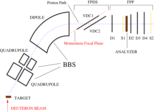
Figure 1: Schematic diagram of the experimental arrangement (top view).

Carbon targets are employed to prepare entangled ${}^{1}S_{0}$ two proton states by ${}^{12}C(d,^{2}He)^{12}B^{*}$ and ${}^{1}H(d,^{2}He)n$ reactions, the latter arising from the hydrogen impurity in the target. The layout of the detector system is shown in Figure 1. From several reactions that occur, the Big Bite Spectrometer (BBS) selects positively charged particles of momenta $p=600\pm 50$ MeV/c. The spectrometer is equipped with a focal plane detector system (FPD) which consists of two planes of drift chambers (VDCs) to determine the momentum of the protons. Behind this system is the focal plane polarimeter (FPP), which consists of four sets of multi-wire proportional chambers (MWPCs), labeled D1-D4, and two sets of plastic scintillator arrays (S1 and S2). A carbon analyzer is placed just next to scintillator S1.

A particle of positive charge and momentum 600 $\pm$ 50 MeV/c entering the spectrometer will leave ionization trails in the VDCs. This causes scintillations in S1. The particle undergoes spin-dependent scattering in the carbon analyzer, leaves ionization trails in the wire chambers and passes through S2. For an event to be registered, we require that a particle would have passed all the way up to S2. The scintillators have an intrinsic time resolution better than 1 ns.

The four momentum vector of the particle is determined by measuring the position and direction of its trajectory in the BBS focal plane by means of the high resolution VDCs and chamber D1. The particle trajectory downstream the analyzer is measured by means of chambers D2-D4. The redundancy of three sets of spatial coordinates upstream and downstream the analyzer ensures a flat detection efficiency.

The data taking logic is set as follows: A hardware coincidence requires that there is a signal between a scintillator in S1 and another in S2, within a time interval of 150 ns. The window is set wide open on purpose. First, the protons travelling along various paths in the spectrometer have different flight times between S1 and S2. More importantly, the cyclotron operates at a frequency of 43 MHz. Taking data in this mode provides a good handle on random coincidences during the off-line analysis, since events separated by more than 20 ns arise due to random coincidences. If this coincidence condition is satisfied, the data from all wire chambers are read out and subject to an online data analysis performed by a set of fast digital signal processors. Events fulfilling the requirements for two coincident protons passing the setup are stored on tape. The TDC data is stored in bins of 1 ns and allow for an event registration over 350 ns, to permit the ion drift times to be recorded. Protons, travelling at speeds of about 0.5c, spend a few nanoseconds in the FPD region and another few nanoseconds in the FPP region. The transit times of the ionization trails in the VDCs and wire chambers are of the order of few hundred nano seconds (drift speeds are of 50 $\mu$m/ns, and drift lengths are about 5 mm). The protons have been out of the entire system long before the trail information is received by the electronic circuitry and processed by the data acquisition system. Since a proton spends a little over 10 picoseconds at each detection element, which generate their signals independent of each other, we believe that the communication between pairs of protons by means other than superluminal signals is not possible.

This standard nuclear physics instrumentation allows the data of each particle track to be recorded providing information on particle identification, its momentum vector, its time relation with respect to other particles in the same event, and its direction after it passes through the carbon analyzer. With the momentum axis of the protons as the reference z-axis, the polarization analysis can be done for any arbitrary set of x-y axes in the analyzer plane, with an acceptance of the entire 180 degrees. We eliminate what is known as trigger bias in subatomic physics and address two loopholes raised by Peres [7] and Redhead[8]: “counterfactuality” and “conscious-observer dependence” of measurements. As we cover the entire angular range for polarization analysis in the x-y plane, the limitation of a single angular setting per particle per event does not arise here. Also, since the orientation of axes is done during the off-line analysis several months after the experiments have been performed, we do not have the problem of the “choice of analyser setting made well in advance of the emission of the particles from the source”[8].

3 Measurement and Data Analysis

In the summer of 2001, we ran the experiment over a three-day period. From a data volume of several tens of millions of triggers, we could identify 4.7 million as two-proton events. The next task was to select the events due to the $(d,^{2}He)$ reaction. We know that, in this reaction, protons in each pair are at rest relative to each other in the center of mass frame. We thus apply standard relativisitic kinematical equations with each event Lorentz boosted to the center of mass frame, and select the events for which the relative kinetic energy of the proton pair is less than 1 MeV, allowing for the instrumental resolution. Figure 2

Figure 2: Sum of the proton-pair kinetic energies in the $(d,^{2}He)$ reaction on ${}^{12}C$ and ${}^{1}H$ for $E_{d}=170$ MeV. The singlet peaks above background are clearly seen.

is a plot of the sum of the kinetic energies of two protons for events thus selected. Noteworthy are the peaks at 170 and 158 MeV, respectively due to ${}^{1}H(d,^{2}He)$ and ${}^{12}C(d,^{2}He)^{12}B$ reactions. The events in these sharp peaks are thus proton pairs due to the decay of a ${}^{2}He$ ${}^{1}S_{0}$ intermediate state.

We follow the fate of each proton in each event as they pass through the carbon analyzer, acquiring the information in the detector systems D1-D4 and S1, S2. First of all, we use only those events where both protons scatter at angles larger than 3 degrees in the carbon analyzer, since the most forward scattering is Coulomb type and it is not spin-dependent. We have a good estimate of the carbon analyzing power from earlier works of KVI groups [9]. It was estimated to be 0.2 for angles 5-20 degrees. We realized that our data provides an inherent measurement of the analyzing power since we deal with proton pairs in which spins of the two protons in each pair are oppositely oriented. Using this information, we were able to deduce the analyzing power for our dynamical range as $A=0.25$. It is quite satisfying to note that this result is in good agreement with the earlier KVI results.

4 Results

We are now in a position to deduce the experimental correlations to compare against the expectations from conventional quantum mechanical arguments and those of Bell[2] and Wigner[4].

4.1 Bell correlations

The formulation of Bell’s inequality finds its basis in the EPRB gedanken experiment of Bohm[10], considering a pair of spin-half particles in the singlet state.

A measurement is made on each particle, determining the projection of its intrinsic spin vector along some arbitrary direction orthogonal to the momenta of the pair. Bell showed that the products of such measurements lead to an experimental condition under which the existence of the hidden parameters could be tested against the completeness of quantum theory.

If $\hat{a}$ and $\hat{a^{\prime}}$ are arbitraty unit vectors along which the spin of the first particle is measured (and $\hat{b}$ and $\hat{b^{\prime}}$ apply similarly to the second particle), the hidden variables framework results in an algebraic condition for the probabilities, $P(\cdot,\cdot)$:

$$|P(\hat{a},\hat{b})-P(\hat{a},\hat{b^{\prime}})+P(\hat{a^{\prime}},\hat{b})+P(\hat{a^{\prime}},\hat{b^{\prime}})|\leq 2.$$ (1)

while the quantum expectation value, $P_{QM}(\theta)$, for these correlation functions is

$$P_{QM}(\theta)=-\cos\theta$$ (2)

where $\theta$ is the angle between the unit vectors $\hat{a}$ and $\hat{b}$. (1) is satisfied for the hidden variables case, but (for certain choices of the co-planar unit vectors) it is violated by (2).

During the off-line analysis (one year after the experiment was performed), we selected eight angular combinations for which the quantum mechanical predictions exceed the Bell limits. The results of this analysis are shown in table 1 and figure 3.

The first observation is the large error due to limited statistics associated with the data. Secondly, the quantum mechanical results for all sets are nearly constant, while the data seems to vary from 0.7 (consistent with Bell’s limit) to about 2.75 (clearly violating the inequality). Needless to say, definitive conclusions await more precise measurements. However, we would like to emphasize that this type of measurement has an excellent potential to settle this problem.

	Bell	Quantum
Case	Inequality	Mechanics	Experiment
1	$P(0^{\circ},25^{\circ})-P(0^{\circ},75^{\circ})+P(50^{\circ},25^{\circ})+P(50^{\circ},75^{\circ})$	2.46	0.67$\pm$	2.30
2	$P(0^{\circ},30^{\circ})-P(0^{\circ},90^{\circ})+P(60^{\circ},30^{\circ})+P(60^{\circ},90^{\circ})$	2.60	1.21$\pm$	2.42
3	$P(0^{\circ},35^{\circ})-P(0^{\circ},105^{\circ})+P(70^{\circ},35^{\circ})+P(70^{\circ},105^{\circ})$	2.72	1.54$\pm$	2.76
4	$P(0^{\circ},40^{\circ})-P(0^{\circ},120^{\circ})+P(80^{\circ},40^{\circ})+P(80^{\circ},120^{\circ})$	2.80	2.11$\pm$	2.86
5	$P(0^{\circ},45^{\circ})-P(0^{\circ},135^{\circ})+P(90^{\circ},45^{\circ})+P(90^{\circ},135^{\circ})$	2.83	2.23$\pm$	2.48
6	$P(0^{\circ},50^{\circ})-P(0^{\circ},150^{\circ})+P(100^{\circ},50^{\circ})+P(100^{\circ},150^{\circ})$	2.79	2.39$\pm$	2.87
7	$P(0^{\circ},55^{\circ})-P(0^{\circ},165^{\circ})+P(110^{\circ},55^{\circ})+P(110^{\circ},165^{\circ})$	2.69	2.58$\pm$	2.91
8	$P(0^{\circ},60^{\circ})-P(0^{\circ},180^{\circ})+P(120^{\circ},60^{\circ})+P(120^{\circ},180^{\circ})$	2.50	2.75$\pm$	2.95

Table 1: Quantum predictions and experimental results for several violating cases of the Bell inequality.

Figure 3: Eight test cases of the experimental data from Table 1 versus quantum predictions and the limit of the Bell inequality.

4.2 Wigner Inequality

The Wigner inequality is similar to Bell’s, but arguably stronger, offering a clearer method of distinguishing between quantum predictions and hidden variables results. This inequality is:

$$P(a,c)_{corr}-P(a,b)_{corr}-P(b,c)_{corr}\leq 0.$$ (3)

$P(\cdot,\cdot)_{corr}$ is the probability that the spin projections of particles one and two are correlated (pointing in the same direction) along their respective measurement axes. The three axes $\hat{a},\hat{b}$ and $\hat{c}$ are co-planar with $\hat{b}$ bisecting the other two. Agreement of the experiment with (3), if observed, would be evidence for the existence of hidden variables, while a positive experimental value would be consistent with the predictions of quantum theory.

We selected six sets of orientations, spanning the entire angular range $0^{\circ}$ to $180^{\circ}$. The results are shown in table 2, and are shown in figure 4. As can be seen, while the data may be consistent with the quantum predictions due to the large errors, there is a clear trend for the results to lie below the zero line, favoring the hidden variables condition. As before, a larger data sample is required to settle this question.

We suggest that for the first time, in a single setting we have obtained data to test both the Bell and Wigner inequalities, covering the entire angular range, thus avoiding the loopholes of observer dependence and counterfactuality. We plan to continue this work with similar tests in the near future.

It is a pleasure to thank P. Busch for valuable discussions. We acknowledge the financial support of KVI and NSERC Canada.

		Experimental
	Wigner Comparison	Result
1	$P(0^{\circ},30^{\circ})-P(0^{\circ},15^{\circ})$	0.20$\pm$	0.78
	$-P(15^{\circ},30^{\circ})$
2	$P(0^{\circ},60^{\circ})-P(0^{\circ},30^{\circ})$	-0.38$\pm$	0.77
	$-P(30^{\circ},60^{\circ})$
3	$P(0^{\circ},90^{\circ})-P(0^{\circ},45^{\circ})$	-0.54$\pm$	0.79
	$-P(45^{\circ},90^{\circ})$
4	$P(0^{\circ},120^{\circ})-P(0^{\circ},60^{\circ})$	-0.71$\pm$	0.81
	$-P(60^{\circ},120^{\circ})$
5	$P(0^{\circ},150^{\circ})-P(0^{\circ},75^{\circ})$	-0.62$\pm$	0.80
	$-P(75^{\circ},150^{\circ})$
6	$P(0^{\circ},180^{\circ})-P(0^{\circ},90^{\circ})$	0.13$\pm$	0.76
	$-P(90^{\circ},180^{\circ})$

Table 2: Results for Wigner Inequality test.

Figure 4: Results of Wigner’s inequality for the six cases of Table 2.

References

- [1] A. Einstein, B. Podolsky and N. Rosen, Physical Review 47 (1935) 777.
- [2] J.S. Bell, Physics 1 (1964) 195; Reviews of Modern Physics 38 (1966) 447.
- [3] A. Vaziri, G.Weihs and A. Zeilinger, Physical Review Letters 89 (2002), 240401.
- [4] E. P. Wigner, Am. J. Physics, 38 (1970) 1005.
- [5] M. Lamehi-Rachti and W. Mittig, Physical Review D 14 (1976) 2543.
- [6] S. Rakers et al, Nuclear Instruments and Methods in Physics Research A481 (2002) 253.
- [7] A. Peres, Quantum Theory: Concepts and Methods, Kluwer, Dordrecht, (1995).
- [8] M. Redhead, Incompleteness, Nonlocality, and Realism, Clarendon, Oxford (1987).
- [9] V. Hannen, Doctoral Thesis, Westfälische Wilhelms-Universität Münster (2001).
- [10] D. Bohm, Quantum Theory, Prentice-Hall, Englewood Cliffs (1951).