Tunneling dynamics in relativistic and nonrelativistic wave equations

Abstract

We obtain the solution of a relativistic wave equation and compare it with the solution of the Schrödinger equation for a source with a sharp onset and excitation frequencies below cut-off. A scaling of position and time reduces to a single case all the (below cut-off) nonrelativistic solutions, but no such simplification holds for the relativistic equation, so that qualitatively different “shallow” and “deep” tunneling regimes may be identified relativistically. The nonrelativistic forerunner at a position beyond the penetration length of the asymptotic stationary wave does not tunnel; nevertheless, it arrives at the traversal (semiclassical or Büttiker-Landauer) time $\tau$. The corresponding relativistic forerunner is more complex: it oscillates due to the interference between two saddle point contributions, and may be characterized by two times for the arrival of the maxima of lower and upper envelops. There is in addition an earlier relativistic forerunner, right after the causal front, which does tunnel. Within the penetration length, tunneling is more robust for the precursors of the relativistic equation.

I INTRODUCTION

Tunneling is a general feature of wave equations: for frequencies below the “cutoff”, wavenumbers become imaginary and the waves evanescent. Even so, it has been mainly discussed for the Schrödinger equation due to the shocking contrast between the behavior of classical and quantum particles. It has been also traditionally examined for stationary conditions, until a paper by Büttiker and Landauer BL82 triggered the interest on its temporal aspects, again, mostly within the framework of the Schrödinger equation.

Tunneling dynamics may be very counterintuitive when compared with the evolution of propagating waves. Defining “tunneling times” has been in particular non trivial in quantum theory (Ref. TQM is a recent and extense multi-author review; for previous reviews see HS89 ; LA90 ; LM94 ; Chiao98 ; Ghose99 ). After twenty years of discussions and many proposals since BL82 , it is clear that different time scales are relevant depending on the experiment, wave feature, or observable quantity investigated. There is thus not a single tunneling time scale, but several; many of them may be obtained, related to each other, and classified systematically by means of a theory that exploits the non-commutability of the operators implied BSM94 .

One of the most important and commonly found scales is the “traversal”, “semiclassical” or “Büttiker-Landauer” time $\tau$. For the dimensionless Schrödinger equation for a particle moving in a constant potential,

$$i\frac{\partial\psi}{\partial t}=-\frac{1}{2}\frac{\partial^{2}\psi}{\partial x^{2}}+\psi,$$ (1)

(all quantities are dimensionless throughout this work except in the discussion of section III), and for a frequency $\omega_{0}<1$, it is given by BL82

$$\tau=\frac{x}{\kappa_{0}},$$ (2)

where

$$\kappa_{0}=[2(1-\omega_{0})]^{1/2}$$ (3)

in Eq. (2) plays the role of a semiclassical “velocity” which increases for deeper and deeper tunneling (i.e. for smaller $\omega_{0}$). $\tau$ is the characteristic time for the transition from sudden to adiabatic regimes in oscillating barriers, and for the spin rotation in a weak magnetic field. A recent and surprising finding is that it is also the time of arrival of the peak of the forerunner that appears, beyond the penetration length of the asymptotic stationary wave, $x>1/\kappa_{0}$, for a “source” with a sharp onset,

$$\psi(x=0,t)=e^{-i\omega_{0}t}\Theta(t),$$ (4)

and

$$\psi(x>0,t<0)=0.$$ (5)

$\Theta(t)$ is the Heaviside function; in the language of electromagnetic wave propagation it is the envelop function of the input pulse, whereas $\omega_{0}$ is the “signal”, “carrier”, or “excitation” frequency. More precisely, the arrival time is $t_{p}^{t}=\tau/3^{1/2}$ if the peak of the density $|\psi(x,t)|^{2}$ is evaluated with respect to $t$ for $x$ fixed MB00 , and $t_{p}^{x}=\tau$ if it is evaluated with respect to $x$ for $t$ fixed VRS02 .

This role of $\tau$ is indeed surprising because that forerunner is not tunneling beyond $1/\kappa_{0}$, where it is predominantly composed by over-the-barrier ($\omega>1$) components MB00 . The importance of $\tau$ is blurred however within the penetration shell, $x<1/\kappa_{0}$, where the arrival of the tunneling peak obeys a different time scale, inversely proportional to $\kappa_{0}^{2}$ rather than to $\kappa_{0}$ gcv01 ; GVDM02 . In the small-$x$ region the arrival time of the peak $t_{p}^{t}$ as a function of $x$ is rather flat in comparison with the (linear in $x$) arrival time of the peak in the large-$x$ region. It actually forms a basin with a minimum, so that the precursor may arrive later at smaller values of $x$ gcv01 ; GVDM02 . Moreover the forerunner does tunnel at small $x$. This is another unexpected result GVDM02 , after so many works where precursors had been always related to an above-the-barrier passage RMA91 ; TKF87 ; APJ89 ; BM96 . Surely no attention had been paid to the small-$x$ region because the analytical approximations based on saddle and pole contributions of the integral defining the solution fail, as discussed below. This region is the easiest to observe though.

Our initial motivation to undertake the present work was to determine if and how the above recent results extend to the relativistic case. Especifically, our aim is to investigate the role played by $\tau$, and the characteristics of the forerunners at large and small $x$ for under-cut-off, unit-step modulated excitations with the relativistic wave equation

$$\left[\frac{\partial^{2}}{\partial t^{2}}-\frac{\partial^{2}}{\partial x^{2}}+1\right]\psi=0,$$ (6)

which is much more accessible experimentally (with waveguides in evanescent conditions Nimtz ; RRSAS01 ; RM02 ) than the Schrödinger equation. These are all aspects that previous studies of relativistic Klein-Gordon equations with evanescent conditions had not explored DL93 ; JLL01 . Some preliminary, partial results on the role of the relativistic $\tau$ may be found in BT ; MB00 .

Note that the stationary equations corresponding to Eqs. (1) and (6) are equal and have equal solutions, but the two cases are not equivalent in the time domain, because the dispersion relations between $\omega$ and $k$ are different,

$$\omega^{2} = 1+k^{2}\;\;\;\;\;\;({\rm relativistic}),$$ (7)

$$\omega = 1+k^{2}/2\;\;({\rm non\,\,relativistic}).$$ (8)

In fact we have found a wealth of qualitative changes with respect to the Schrödinger scenario as the following sections will show. One of them is discussed in section II, namely, the absence for the relativistic equation of the scaling properties that simplify the nonrelativistic solutions; this implies that qualitatively different solutions are possible for different carrier frequencies in the relativistic case. Section III deals with possible physical realizations of the formalism. The technical tools used are an analytical series expression for the exact solution, which is obtained in section IV, and the asymptotic analysis of section V, based on previous work by Büttiker and Thomas BT , that will allow to describe and understand the wave behaviour at “large-$x$” in simple terms. For small-$x$ this analysis is substituted by numerical exploration in section VI, except in the proximity of the very first front or “causal limit” at $t=x$, where a simple analytical approximation is again available.

II Scaling properties

The solution of Eqs. (6) or (1) with the boundary condition of Eq. (4) is given in both cases by

$$\psi(x,t;\omega_{0})=\frac{i}{2\pi}\int_{-\infty}^{\infty}d\omega\,\frac{e^{ikx-i\omega t}}{\omega-\omega_{0}+i0},$$ (9)

as may be checked by substitution. We shall only consider $x>0$. It is easy to see from Eq. (9) that the wave vanishes for $t<x$. In the relativistic case $k=(\omega^{2}-1)^{1/2}$ is defined with two branch cuts from $\omega=\pm 1$ downwards in the complex $\omega$-plane, as shown in Figure 1, whereas for the nonrelativistic equation, $k=[2(\omega-1)]^{1/2}$ is defined with only one branch cut downwards from $\omega=1$. For evanescent waves, i.e., when $k=i\kappa$, $\kappa>0$ the relativistic wavenumber tends to the nonrelativistic one as $\omega\to 1$,

$$\kappa=(1-\omega^{2})^{1/2}\to_{\omega\to 1}[2(1-\omega)]^{1/2}.$$ (10)

In the nonrelativistic case it is useful to shift the frequency axis by defining the variable

$$\Omega=\omega-1$$ (11)

(in particular $\Omega_{0}=\omega_{0}-1$). Let us also define $\phi(x,t;\Omega_{0})\equiv e^{it}\psi(x,t;\omega_{0})$. If we introduce a scale factor

$$\Omega=\alpha\Omega^{\prime},\;\;\alpha>0,$$ (12)

it follows from Eq. (9) that

$$\phi(x,t;\Omega_{0})=\phi(\alpha^{1/2}x,\alpha t;\Omega_{0}/\alpha),$$ (13)

which means, in words, that any two solutions with excitation frequency above cut-off ($\Omega_{0}>0$) are related to each other by the scaling law of Eq. (13) and similarly, all solutions below cut-off ($\Omega_{0}<0$) are also simply related to each other by scaling. We can generate all possible solutions from two of them, one below and one above cut-off. Nevertheless, Eq. (13) does not hold for the relativistic wave equation because of the different dispersion relation, so that solutions for different excitation frequencies $\omega_{0}$ cannot reduce to each other; they may and do change qualitatively when sweeping over $\omega_{0}$, as demonstrated in Section IV.

III Physical realizations

Even though we use throughout the paper dimensionless variables and equations, it is worth noting that Eq. (6) leads to the Klein-Gordon equation for spin-0 particles by means of the substitutions

$$x = X(m_{0}c)/\hbar,$$ (14)

$$t = Tm_{0}c^{2}/\hbar,$$ (15)

where $X$ and $T$ denote dimensional position and time, and $m_{0}$ and $c$ are the particle’s rest mass and the velocity of light in vacuum. Another interesting connection, much more promising to implement the present analysis experimentally RM02 , and free from the conceptual puzzles of the former, may be established with the equation that governs the electromagnetic field components in waveguides of general constant cross section with perfectly conducting walls Kristensson95 . This requires the substitutions

$$x = X\lambda,$$ (16)

$$t = T\lambda c,$$ (17)

where $\lambda>0$ is one of the eigenvalues of the waveguide.

Dimensional Schrödinger equations corresponding to Eq. (1) may be obtained formally in the limit $c\to\infty$ (the proper one from the Klein-Gordon equation for particles, and an analogous one from the waveguide equation). Physically, the solution of the dimensionless wave equation approaches the solution of the dimensionless Schrödinger equation when it is dominated by $\omega$-components close to one (the cut-off), note that the relativistic dispersion relation, Eq. (7), tends to the nonrelativistic one, Eq. (8), as $\omega\to 1$. Indeed excitations with $\omega_{0}\approx 1$ provide relativistic solutions very close to the nonrelativistic ones except in the region near the causal limit $t=x$ (the “first precursor”), where the whole frequency range of the source signal has a significant influence.

In order to compare relativistic and nonrelativistic equations the same “excitation” will be used, Eq. (4), which for the waveguide may be understood as a compact representation of (real) sine and cosine excitations. Since for the relativistic equation the excitations $e^{\pm i\omega_{0}t}\Theta(t)$ produce at $x$ the complex conjugate wave of each other, only the interval $0<\omega_{0}<1$ will be examined. Also, to carry out the comparison with the Schrödinger equation in terms of analogous quantities, we shall study $|\psi|^{2}$ which, in the relativistic-waveguide case may be simply regarded as the sum of the squares of the waves resulting from the sine and cosine excitations. Because of its meaning in the Schrödinger equation, we shall refer to this quantity as the “density”, even in the relativistic case. The agreement between the relativistic and nonrelativistic solutions near the cut-off and far from $t=x$, combined with the scaling property of Eq. (13) may serve in practice to simulate in a waveguide the solution of the Schrödinger equation for any $\omega_{0}$ in the time domain.

Figure 1: Steppest descent paths in the complex $\omega$ plane for $t=1.5$, $\omega_{0}=0.85$ and $x=1$ (narrow solid line). The thicker solid lines are the two branch cuts while the verticals lines are the asymptotes. The dots mark $\pm\omega_{s}$ and $\pm 1/\omega_{s}$; the cross is at $\omega_{0}$.

IV Relativistic series solution

In this section we shall obtain the solution of Eq. (6) in series form. It will be used to provide exact numerical results as well as analytical approximations for $x,t>0$ and for the sharp onset source of Eq. (4), following refs. gcv99 ; vjpa00 . We begin by Laplace transforming the equation (6) using the standard definition,

$$\overline{\psi}(x;s)=\int\nolimits_{0}^{\infty}\psi(x,t)e^{-st}dt.$$ (18)

The Laplace transformed solution reads,

$$\overline{\psi}(x;s)=c_{1}e^{-px},\qquad x\geq 0,$$ (19)

where we have defined $p=(s^{2}+1)^{1/2}$. The corresponding Laplace transform of Eq. (4), yields,

$$\overline{\psi}(0;s)=\frac{1}{s+i\omega_{0}}.$$ (20)

By combining Eqs. (19) and (20) evaluated at $x=0$ we can determine the value of the constant $c_{1}$,

$$\overline{\psi}(x;s)=\frac{e^{-px}}{s+i\omega_{0}},\qquad x\geq 0.$$ (21)

The time dependent solution for $x>0$ is obtained by performing the inverse Laplace transform of Eq. (21), using the Bromwich integral formula,

$$\psi(x,t)=\frac{1}{2\pi i}\int\limits_{\gamma^{\prime}-i\infty}^{\gamma^{\prime}+i\infty}\overline{\psi}(x;s)e^{st}ds,\qquad t>0,$$ (22)

where the integration path is taken along a straight line $s=\gamma^{\prime}$ parallel to the imaginary axis in the complex $s$-plane. The real parameter $\gamma^{\prime}$ can be chosen arbitrarily as long as all singularities remain to the left-hand side of $s=\gamma^{\prime}$.

To avoid dealing with the branch points at $s=\pm i$ in Eq. (22), let us introduce the change of variable, $-iu=(s+p)$. Thus, $p=i(u^{-1}-u)/2$, and the integral may be written as

$$\psi(x,t)=\frac{1}{2\pi i}\int\limits_{i\gamma-\infty}^{i\gamma+\infty}\Phi(u)du,$$ (23)

where the new integrand $\Phi(u)$ is given by

$$\Phi(u) = \frac{(1-u^{2})}{u(u-\omega_{0}-k_{0})(u-\omega_{0}+k_{0})}$$ (24)

$$\times\text{exp}\{i[u(x-t)-u^{-1}(x+t)]/2\},$$

and $k_{0}=k(\omega_{0})$. The integrand has now an essential singularity at $u=0$ and two simple poles $u_{\pm}=(\omega_{0}\pm k_{0})$. For $x>t$ we close the integration path from above, by a large semicircle $\Gamma_{1}$ of radius $R$, forming a closed contour $C_{1}$. The contribution along $\Gamma_{1}$ vanishes as $R\rightarrow\infty$, and since there are no poles enclosed inside $C_{1},$ $\psi(x,t)=0$ for $x>t$. For the case $x<t,$ we close the integration path from below with a large semicircle $\Gamma_{2}$. The closed contour $C_{2}$ contains three small circles $C_{0,}$ $C_{+}$ and $C_{-}$ enclosing the essential singularity at $u=0$ and the simple poles at $u_{+}$ and $u_{-},$ respectively. Hence, it follows that,

$$\frac{1}{2\pi i}\left[\int\limits_{i\gamma-\infty}^{i\gamma+\infty}-\int\limits_{\Gamma_{2}}+\int\limits_{C_{0}}+\int\limits_{C_{+}}+\int\limits_{C_{-}}\right]\Phi(u)du=0.$$ (25)

The integrals corresponding to the contours $C_{+}$ and $C_{-}$ can be easily evaluated,

$$-\frac{1}{2\pi i}\int\limits_{C_{\pm}}\Phi(u)du=e^{(\pm k_{0}x-i\omega_{0}t)}.$$ (26)

The contour integration for $C_{0}$ involves an essential singularity at $u=0$. Introducing the change of variable $v=-iu\xi^{-1}$ the integral becomes

$$-\frac{1}{2\pi i}\int\limits_{C_{0}}\Phi(u)du=\frac{1}{2\pi i}\int\limits_{C_{0}^{{}^{\prime}}}\frac{1}{\xi^{2}}\frac{(1+v^{2}\xi^{2})e^{\eta(v-v^{-1})/2}}{v(v-v_{+})(v-v_{-})}dv,$$ (27)

where

$$v_{\pm} = z_{\pm}/i\xi,$$ (28)

$$z_{\pm} = (\omega_{0}\pm k_{0}),$$ (29)

$$\xi = \left[(t+x)/(t-x)\right]^{1/2},$$ (30)

$$\eta = (t^{2}-x^{2})^{1/2}.$$ (31)

The integration is carried out by first separating the integrand into partial fractions, and then substituting the formula for the Bessel generating function,

$$e^{\eta(v-v^{-1})/2}=\sum_{n=0}^{\infty}v^{n}J_{n}(\eta)+\sum_{n=1}^{\infty}(-1)^{n}v^{-n}J_{n}(\eta),$$ (32)

and the series expansion,

$$(v_{\pm}-v)^{-1}=(v_{\pm})^{-1}\sum_{n=0}^{\infty}(v/v_{\pm})^{n}.$$ (33)

Now we can calculate the resulting integrals by means of the residue theorem. For the case of an essential singularity, the residue may be determined by computing explicitly the coefficient corresponding to $v^{-1}$ from the series expansion and their products. In that case, equation (27) becomes,

$$-\frac{1}{2\pi i}\int\limits_{C_{0}}\Phi(u)du = \left[-J_{0}(\eta)-\sum_{n=1}^{\infty}(-1)^{n}\frac{J_{n}(\eta)}{(v_{+})^{n}}\right.$$ (34)

$$\left.-\sum_{n=1}^{\infty}(-1)^{n}\frac{J_{n}(\eta)}{(v_{-})^{n}}\right].$$

Finally, by feeding the results given by Eqs. (26) and (34) into Eq. (25), the solution for the internal region reads

$$\psi(x,t)=\left\{\begin{array}[]{ll}\psi(x,k_{0},t)+\psi(x,-k_{0},t),&t>x\\ 0,&t<x,\end{array}\right.$$ (35)

with $\psi(x,\pm k,t)$ defined as

$$\psi(x,\pm k_{0},t) = e^{(\pm ik_{0}x-i\omega_{0}t)}+\frac{1}{2}J_{0}(\eta)$$ (36)

$$-\sum\limits_{n=0}^{\infty}(\xi/iz_{\pm})^{n}J_{n}(\eta).$$

It is worthwhile to remark the similarity of the above solution with that of Eq. (16) of ref. gcv99 and Eqs. (15) and (16) of ref. vjpa00 . From Eq. (32),

$$\sum\limits_{n=0}^{\infty}(\xi/iz_{\pm})^{n}J_{n}(\eta)=e^{i[\pm k_{0}x-\omega_{0}t]}-\sum\limits_{n=1}^{\infty}(-1)^{n}(iz_{\pm}/\xi)^{n}J_{n}(\eta).$$ (37)

Therefore, Eq. (36) may also be written in the form

$$\psi(x,\pm k_{0},t)=\frac{1}{2}J_{0}(\eta)+\sum\limits_{n=1}^{\infty}(-1)^{n}(iz_{\pm}/\xi)^{n}J_{n}(\eta),$$ (38)

which will be useful for the analysis of the region close to the causal limit $t=x$.

The above relativistic solutions should be contrasted with the solution to the nonrelativistic equation using the same initial condition MB00 ; VRS02 ,

$$\psi(x,t)=\frac{1}{2}{\rm e}^{-it}{\rm e}^{ix^{2}/(2t)}[w(y_{k_{0}})+w(y_{-k_{0}})]$$ (39)

where $w(y_{\pm k_{0}})$ stands for the “$w$-function” as with argument $y_{\pm k_{0}}$,

$$y_{\pm k_{0}}=i{\rm e}^{-i\pi/4}\left(\frac{1}{2t}\right)^{1/2}\left[x\mp k_{0}t\right].$$ (40)

V Saddle-pole approximation for large $x$

Following Sommerfeld and Brillouin SB , who studied the propagation of a unit step-function modulated signal in a Lorentz medium, the forerunners and other wave features may be understood and quantify with asymptotic analysis techniques. Let us deform the integral of Eq. (9) along the steepest descent paths (SDP), see Figure 1, defined by

$$\omega_{I}^{\pm}=\frac{-(\pm\omega_{R}\omega_{s}-1)(\pm\omega_{R}-\omega_{s})}{[(\omega_{s}^{2}-1)(-\omega_{R}^{2}\pm 2\omega_{R}\omega_{s}-1)]^{1/2}}$$ (41)

($\omega_{R}$ and $\omega_{I}$ are the real and imaginary parts of $\omega$), where the upper sign is for the positive saddle at $\omega_{s}$ and the lower sign for the negative saddle at $-\omega_{s}$,

$$\pm\omega_{s}=\pm\frac{t}{(t^{2}-x^{2})^{1/2}},$$ (42)

plus a clockwise circle around the pole at $\omega_{0}$ that must be added to the contour if the pole has been crossed by the SDP. The SDP have asymptotes at $\omega_{R}=\pm[\omega_{s}\pm(\omega_{s}^{2}-1)^{1/2}]$ and cross the real axis at $\pm\omega_{s}$ and $\pm\omega_{s}^{-1}$, see figure 1. The crossing of the pole occurs when $\omega_{s}^{-1}=\omega_{0}$, i.e., for fixed $x$, at time

$$\tau=\frac{x}{\kappa_{0}}=\frac{x}{(1-\omega_{0}^{2})^{1/2}},$$ (43)

which generalizes the traversal time of Eq. (2) for the relativistic case BT . Note that $\tau>x$, i.e., the crossing occurs always after the arrival of the first front imposed by relativistic causality at $t=x$. One might be tempted to believe that the crossing of the pole is associated with the arrival of a “monochromatic” $\omega_{0}$-front Stevens . That this is not the case has been pointed out in several works on the Schrödinger equation, the reason being the dominance of over-the-barrier components associated with the saddle. The frequency analysis of the relativistic forerunner is more complex as the following discussion will demonstrate.

Applying the standard asymptotic approximation for the saddle contributions BH86 , $\psi$ takes the form

$$\psi(x,t) \approx \psi_{p}+\psi_{s}^{+}+\psi_{s}^{-},$$ (44)

$$\psi_{p} = \Theta(t-\tau)e^{-\kappa_{0}x}e^{-i\omega_{0}t},$$ (45)

$$\psi_{s}^{\pm} = i\sqrt{\frac{\mp ix^{2}}{2\pi t^{2}}}\frac{\omega_{s}}{\omega_{s}\mp\omega_{0}}\exp[\mp i\eta].$$ (46)

Eq. (44) is a good approximation as long as the “width” of the saddle is small compared to the “distance” from the saddle to the pole BT ,

$$(\omega_{s}\mp\omega_{0})^{2}\frac{\partial^{2}\phi}{\partial\omega^{2}}\bigg{|}_{\omega=\omega_{s}}=\frac{\eta^{3}}{x^{2}}(\omega_{s}\mp\omega_{0})^{2}>>1,$$ (47)

where $\phi=\omega t-kx$. This always happens for large enough $t$ and fails very close to $t=x$. Applying this condition at $t=\tau$ we get

$$x\omega_{0}\kappa_{0} >> 1\;\;({\rm positive\;saddle}),$$ (48)

$$x\omega_{0}(1+\omega_{0}^{2})^{2}/\kappa_{0}^{3} >> 1\;\;({\rm negative\;saddle}),$$ (49)

to be compared with the simpler nonrelativistic criterion MB00

$$x\kappa_{0}>>1.$$ (50)

At variance with the nonrelativistic case, the condition of Eq. (49) may only worsen with decreasing $\omega_{0}$, whereas the one in Eq. (48) improves from $\omega_{0}=1$ up to the critical value $\omega_{0}=(1/2)^{1/2}\approx 0.7$, but also worsens below. $\psi_{s}^{+}$ is dominant with respect to $\psi_{s}^{-}$ as $\omega_{0}\to 1$ and for large t but the importance of the negative saddle increases with decreasing $\omega_{0}$ and t,

$$\frac{|\psi_{s}^{+}|}{|\psi_{s}^{-}|}=\frac{t+\eta\omega_{0}}{t-\eta\omega_{0}}.$$ (51)

In particular, at $t=\tau$,

$$\frac{|\psi_{s}^{+}|}{|\psi_{s}^{-}|}=\frac{1+\omega_{0}^{2}}{1-\omega_{0}^{2}}.$$ (52)

To compare the relative importance of the saddle and pole contribution we can examine the ratio $\left|\psi_{p}/\psi_{s}^{+}\right|$,

$${\cal R}(x,t) = \frac{|\psi_{p}|}{|\psi_{s}^{+}|}=\pi e^{-2\kappa_{0}x}\frac{t^{2}\eta}{x^{2}}$$ (53)

$$\times \left(1-\frac{\omega_{0}\eta}{t^{2}}\right)\Theta(t-\tau).$$

${\cal R}(t,x)$ grows monotonously with $t$ and decreases with $x$. The time scale for the attainment of the stationary regime, or equivalently, the duration of the transient regime dominated by the saddles before the pole dominates, $t_{tr}$, can be identified as the time when ${\cal R}=1$. Assuming that $\tau\ll t_{tr}$, this time is given by

$$t_{tr}=\frac{e^{{2\kappa_{0}x}/{3}}x^{2/3}}{(2\pi)^{1/3}(1-\omega_{0})^{2/3}},$$ (54)

which is an exponentially large quantity as in the Schrödinger equation MB00 . Indeed, Eq. (54) tends to the nonrelativistic result taking $\omega_{0}\to 1$.

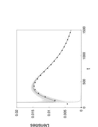
Figure 2: $|\psi_{s}^{+}|^{2}$(solid black line), $|\psi_{s}^{-}|^{2}$ (dashed line) and $|\psi_{s}^{+}+\psi_{s}^{-}|^{2}$ (solid grey line); $|\psi_{s}|^{2}$ (nonrelativistic: dots). $x=100$ and $\omega_{0}=0.99$.

V.1 “Densities”

If the pole contribution is negligible compared to the two saddle point contributions, the total density is given by

$$|\psi(x,t)|^{2}\approx|\psi_{s}^{+}+\psi_{s}^{-}|^{2}=$$ (55)

(56)

$$\frac{t^{2}+\omega_{0}^{2}\eta^{2}+x^{2}(t^{2}/\tau^{2}+\omega_{0}^{2})\sin(2\eta)}{\pi\eta x^{2}\left(t^{2}/\tau^{2}+\omega_{0}^{2}\right)^{2}},\;\;{\cal R}\ll 1$$ (57)

Figure 3: Upper (a) and lower (b) envelops at at $x=100$ for : $\omega_{0}=0.99$ (solid line), $\omega_{0}=0.97$ (dashed line) and $\omega_{0}=0.5$ (long-dashed line).

Figure 4: $t_{max}^{x,U}/\tau$ (dashed line); $t_{min}^{x,U}/\tau$ (solid line); $t_{max}^{t,U}/\tau$ (dotted-dashed line); $t_{min}^{t,U}/\tau$ (dotted line); $t_{max}^{x,L}/\tau$ (circles), and $t_{max}^{t,L}/\tau$ (crosses)

.

The interference between the two saddles leads to an oscillatory pattern of the density, whose amplitude $A$ increases for deeper tunneling, see Figure 2. From Eq. (57),

$$A=\frac{x^{2}}{\pi\eta(t^{2}-\omega_{0}^{2}\eta^{2})}.$$ (58)

The oscillation only disappears in the nonrelativistic limit $\omega_{0}\to 1$, $t>>x$.

Since the dominant frequencies of the saddle terms for $\psi_{s}^{+}$ and $\psi_{s}^{-}$ are $\pm\omega_{s}$ respectively, the oscillation period of the interference pattern between the two saddles is very well approximated by $\pi/\omega_{s}$. Of course, beyond $t_{tr}$ the oscillations fade away and are substituted by the asymptotic dominance of the pole term.

The upper and lower envelops of $|\psi_{s}^{+}+\psi_{s}^{-}|^{2}$ are given, from Eq. (57), by:

$$|\psi_{s}^{+}+\psi_{s}^{-}|^{2}_{U}=\frac{2t^{2}}{\pi x^{2}\eta\left(t^{2}/\tau^{2}+\omega_{0}^{2}\right)^{2}},$$ (59)

$$|\psi_{s}^{+}+\psi_{s}^{-}|^{2}_{L}=\frac{2\omega_{0}^{2}\eta}{\pi x^{2}\left(t^{2}/\tau^{2}+\omega_{0}^{2}\right)^{2}}.$$ (60)

A second forerunner, after the first one at $t=x$, may thus be identified thanks to the maxima of these envelops, see Fig. 2. The upper envelop may hold a maximum and a minimum, but they disapear below a critical value of the injection frequency $\omega_{0}$, see Fig. 3 a. We may thus clearly distinguish between shallow and deep tunneling regimes with qualitatively different features for the upper envelop. On the other hand, the lower envelop has only a maximum that remains for any $\omega_{0}$, although its amplitude decreases with smaller $\omega_{0}$, see Eq. (60) and Fig. 3 b, and becomes physically irrelevant in comparison to the upper envelop.

Taking the derivative with respect to $t$ or $x$ of the envelops, we can extract “temporal” or “espacial extrema” respectively. In the case of the lower envelop,

$$t_{max}^{x,L} = \frac{\tau}{2}\left[{3-\omega_{0}^{2}+\sqrt{9(1+\omega_{0}^{4})-14\omega_{0}^{2}}}\right]^{1/2},$$

$$t_{max}^{t,L} = \left(\frac{4-3\omega_{0}^{2}}{3}\right)^{1/2}\tau,$$ (61)

which are always larger than the corresponding nonrelativistic limits, $\tau$ and $\tau/\sqrt{3}$ respectively. For the upper envelop we obtain

$$t_{max/min}^{t,U} = \frac{\tau}{\sqrt{6}}\left[2-\omega_{0}^{2}\pm\sqrt{4-28\omega_{0}^{2}+25\omega_{0}^{4}}\right]^{1/2},$$

$$t_{max/min}^{x,U} = \frac{\tau}{2}\left[1+\omega_{0}^{2}\pm\sqrt{1-22\omega_{0}^{2}+25\omega_{0}^{4}}\right]^{1/2}.$$ (62)

The ratios between the above critical times and $\tau$, $t_{ext}/\tau$ are represented in Figure 4. None of these ratios depend on $x$. This is explained by an interesting scaling property of the envelops (which is also satisfied separately by $|\psi_{s}^{\pm}|^{2}$),

$$\alpha |\psi_{s}^{+}(\alpha x,\alpha t)+\psi_{s}^{-}(\alpha x,\alpha t)|^{2}_{U/L}$$ (63)

$$= |\psi_{s}^{+}(x,t)+\psi_{s}^{-}(x,t)|_{U/L}^{2}$$

which holds for any fixed excitation energy and has been also noted in the nonrelativistic saddle contribution to the density VRS02 . A consequence is that the maxima and minima of the envelops with respect to $x$ and $t$ travel at constant velocity, which may only depend on $\omega_{0}$. Nevertheless, when the interference is taken into account a similar relation is not satisfied by Eq. (57). Equation (42) implies that $\omega_{s}$, and therefore the oscillation period of the density oscillations, remain constant when $x$ and $t$ are scaled, instead of increasing as the time span of the forerunners does.

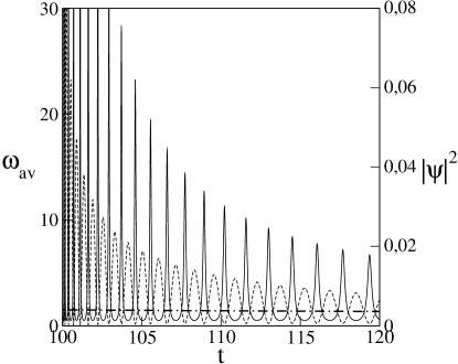
Figure 5: $|\psi|^{2}$ and $\omega_{av}$ versus time for $x=100$ and $\omega_{0}=0.5$ (dashed line and solid line respectivity). Also shown is the nonrelativistic $\omega_{av}$ (dotted-dashed line).

V.2 Instantaneous frequency

Figure 5 shows a typical probability density for the first forerunner region at large $x$, where the two saddle contributions dominate clearly over the pole contribution. We have choosen a signal frequency $\omega_{0}=0.5$ and a fixed position $x=100$ ($\tau\approx 710$). In this scale, there are no differences between the exact and the aproximate solution in Eq. (44) except in the very limit $t=x$. In the same figure we have plotted the average local instantaneous frequency $\omega_{av}\equiv-Im[\left(\partial{\psi}/\partial t\right)/\psi]$ versus time Cohen95 ; MB00 . Since now $\psi\approx\psi^{+}_{s}+\psi_{s}$ we obtain,

$$\omega_{av}=\frac{\omega_{0}\left(-2t^{2}y+x^{2}\cos(2y)\right)}{\eta\left[-t^{2}-\omega_{0}^{2}\eta^{2}+(-t^{2}+\omega_{0}^{2}\eta^{2})\sin(2y)\right]},$$ (64)

with envelops

$$\omega_{av}^{U}=\frac{t^{2}}{\omega_{0}\eta^{2}},\;\;\;\;\omega_{av}^{L}=\omega_{0}.$$ (65)

The density and $\omega_{av}$ are dephased. In particular the maxima of the density correspond to the minima at $\omega_{0}$ of the frequency, so that most of the density corresponds to frequencies below the cut-off. (This effect is more and more clear for lower injection frequencies.) This means that the first forerunner is essentially tunneling whereas, in the same time domain, the nonrelativistic wave is not. For the second forerunner, however, the minima of the density are not so close to zero, see e.g. Figure 2, so that there is an alternating influence of frequencies above and below cut-off.

VI Exact solution for small $x$

The small $x$ region may be defined by the failure of the inequalities in Eqs. (48) and (49). It requires in general an exact numerical treatment because the simple saddle-pole aproximation is not valid anymore. Figure 6 exhibits a plot of the “density” as a function of time, for given values of $x$ and $\omega_{0}$, near $\eta\approx 0$ using Eq. (38). The exact calculation (solid line) exhibits a sharp relativistic wavefront, reaching unity at $x=t$, followed by mild oscillations of smaller amplitude and eventually by the asymptotic stationary density. Figure 6 provides also a comparison with the one-term approximation (dashed line) to Eq. (38), namely,

$$\psi(x,t)\approx J_{0}(\eta)-2i\frac{\omega_{0}}{\eta}J_{1}(\eta).$$ (66)

One sees that the above approximation gives an excellent description in the vicinity of the relativistic wavefront.

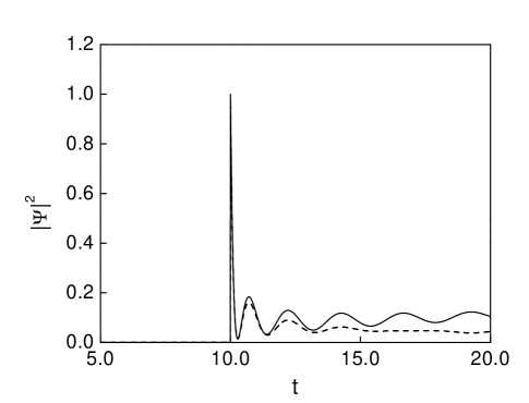
Figure 6: $|\psi|^{2}$ versus time at $x=10$ and $\omega_{0}=0.99$ for the exact calculation (solid line) and the first term approximation (dashed line).

In Figure 7, we have plotted the “density” versus time for three different values of $\omega_{0}$. The first forerunner just after $t=x$ may be characterized from the expansion of the two Bessel functions in Eq. (66) for very small $\eta$ as ,

$$\psi(x,t)\approx 1-(t-x)\left[-i\frac{\omega_{0}}{2}-\frac{t+x}{4}\right].$$ (67)

Figure 7: $|\psi|^{2}$ versus time at $x=0.1$ for three differents values of $\omega_{0}$: $\omega_{0}=0.99$ (solid line), $\omega_{0}=0.8$ (dotted line) and $\omega_{0}=0.1$ (dotted-dashed line). The same quantity is plotted for the nonrelativistic solution (dashed line, $\omega_{0}=0.99$; long dashed line, $\omega_{0}=0.8$, and circles for $\omega_{0}=0.1$).

Figure 8: $\omega_{av}$ versus time at $x=0.1$ for two differents values of the injection frequency: $\omega_{0}=0.99$ (solid line), $\omega_{0}=0.1$ (dotted line). The same quantity is plotted for the nonrelativistic solution (dashed line) for $\omega_{0}=0.99$ and long dashed line for $\omega_{0}=0.1$. The axis has been cut to show all curves with the same scale.

Figure 9: time of arrival of the maximum of the lower envelop for the relativistic case (dots) and for the first forerunner in the nonrelativistic case (solid line). $\omega_{0}$ has been choosen equal to 0.98.

Figure 10: $t_{p_{min}}$ versus $1/\kappa_{0}^{2}$ using $\omega_{0}$ from 0.95 to 0.999.

It consists of a peak that decays from 1 with slope $-(t+x)/2$ independently of $\omega_{0}$. At variance with the nonrelativistic equation, that immediately smoothes away any initial singularity, the relativistic equation propagates the sharp jump of the excitation in the input signal. Note in Figure 7 that for deeper tunneling the asymptotic relativistic signal becomes stronger than the non relativistic one: the pole contribution to the density has the same form in both cases MB00 , $e^{-2\kappa_{0}}$, but the $\kappa_{0}$’s are only equal at $\omega_{0}=0$. Otherwise, $\kappa_{0}$ (nonrelativistic) $>\kappa_{0}$ (relativistic) for $0<\omega_{0}<1$.

In fact, the approximation in Eq. (67) is valid for any value of $x$, but its relevance is mostly appreciated at small $x$. At large $x$ the first peak is immediately followed by rapid oscilations of large amplitude, so that the first forerunner is characterized better by the upper envelop in that case, except in the immediate proximity of the causal limit.

The average local instantaneous frequency at the causal limit $x=t$ is always $\omega_{0}$, see Figure 8 and Eq. (67), which is quite different from the “high” frequencies of the nonrelativistic case, see Figure 8 ($\omega_{av}(t=x;$ nonrelativistic$)=1.5$ for $\omega_{0}=0.99$). In fact the first precursor as well as the rest of the wave tunnel cleanly at any time if the source frequency is small enough. This limit value of $\omega_{0}$ for total tunneling decreases when $x$ increases.

We may define as before the second forerunner according to some convention. Numerically it is relatively simple to identify the maximum of a lower envelop for $\omega_{0}\gtrsim 0.8$. Figure 9 shows that, as in the nonrelativistic case, we have a region where the signal arrives at earlier times at greater $x$, but for large $x$ it grows linearly with $x$. The arrival time of the envelop’s peak at the minimum of the basin, $t_{p_{min}}$, depends linearly on $1/\kappa_{0}^{2}$, see Figure 10, as in the nonrelativistic case.

VII Summary and discussion

In this work we have described the forerunners and the transition to the asymptotic regime of the solution of a relativistic wave equation for a unit-step-function modulated input signal with carrier frequencies below cut-off. This extends the investigation carried out previously for the Schrödinger equation MB00 ; VRS02 ; GVDM02 , with the bonus that the relativistic equation may be physically implemented in waveguides. The main differences between the relativistic and nonrelativistic cases are: (a) the relativistic solutions are not simply related to each other by time and position scaling as in the nonrelativistic case, so that qualitatively different “shallow” and “deep” tunneling regimes may be distinguished; (b) tunneling is more robust relativistically, both in the precursors and asymptotically; (c) the “first” relativistic precursor, right after the limit imposed by causality does not have a nonrelativistic counterpart, and does tunnel; (d) the “second” precursor, which tends to the nonrelativistic one for excitation frequencies near cut-off, has an oscillating structure that may be characterized by its envelops. The traversal time $\tau$ is not an exact measure of their arrival except in the nonrelativistic limit.

While the emphasis here has been on the comparison between the results of the Schrödinger and the relativistic wave equation for a canonical input signal, our next objective is to incorporate to the theory more elements relevant for the waveguide experiments, such as dissipation, other forms of input envelop pulses (e.g. square or Gaussian), waveguides with section constraints or barriers of lower dielectric constant Ermig96 (for classically forbidden regions of finite width, the nonrelativistic descriptiongcv01 ; gcv03 exhibits also the “shallow” and “deep” tunneling regimes mentioned above), frequency band-limitations, and a separate analysis of cosine or sine excitations, which have been combined here to relate directly the relativistic wave amplitudes to the nonrelativistic densities.

- (1) M. Büttiker and R. Landauer, Phys. Rev. Lett. 49, 1739 (1982).
- (2) Time in Quantum Mechanics ed. by J. G. Muga, R. Sala and I. L. Egusquiza (Springer, Berlin, 2002)
- (3) E.H. Hauge, J.A. Stovneng, Rev. Mod. Phys. 61, 917 (1989).
- (4) C.R. Leavens, G.C. Aers, in Scanning Tunneling Microscopy and Related Techniques, ed. by R. J. Behm, N. García, H. Rohrer (Kluwer, Dordrecht, 1990)
- (5) R. Landauer and Th. Martin, Rev. Mod. Phys. 66, 217 (1994).
- (6) R. Y. Chiao and A. M. Steinberg, Progress in Optics 37, 345 (1997).
- (7) P. Ghose, Testing Quantum Mechanics on New Ground (Cambridge University Press, Cambridge, 1999), Chapter 10.
- (8) S. Brouard, R. Sala and J. G. Muga, Phys. Rev. A 49, 4312 (1994).
- (9) J. G. Muga and M. Büttiker, Phys. Rev. A 62, 023808 (2000).
- (10) J. Villavicencio, R. Romo and S. S. Silva, Phys. Rev. A. 66 042110 (2002).
- (11) G. García-Calderón and J. Villavicencio, Phys. Rev. A 64 012107 (2001).
- (12) G. García-Calderón, J. Villavicencio, F. Delgado and J. G. Muga, Phys. Rev. A 66 042119 (2002).
- (13) A. Ranfagni, D. Mugnai and A. Agresti, Phys. Lett. A 158, 161 (1991).
- (14) N. Teranishi, A. M. Kriman and D. K. Ferry, Superlattices and Microstructures, 3, 509 (1987).
- (15) A. P. Jauho and M. Jonson, Superlattices and Microstructures 6, 303 (1989).
- (16) S. Brouard and J. G. Muga, Phys. Rev. A 54, 3055 (1996).
- (17) A. Enders and G. Nimtz, J. Phys. (Paris) I 2, 1693 (1992); Phys. Rev. E 48, 632 (1993).
- (18) A. Ranfagni, R. Ruggeri, C. Susini, A. Agresti, P. Sandri, Phys. Rev. E 63 025102-1 (2001).
- (19) D. Mugnai and A. Ranfagni, in Time in Quantum Mechanics ed. by J. G. Muga, R. Sala and I. L. Egusquiza (Springer, Berlin, 2002).
- (20) J. M. Deutch and F. E. Low, Annals of Physics 228, 184 (1993)
- (21) A. D. Jackson, A. Lande, and B. Lautrup, Phys. Rev. A 64, 044101 (2001)
- (22) M. Büttiker and H. Thomas, Ann. Phys. (Leipzig) 7, 602 (1998); Superlattices Microstruct. 23, 781 (1998).
- (23) G. Kristensson, J. Electro. Waves Applic. 9, 641 (1995).
- (24) G. García-Calderón, A. Rubio and J. Villavicencio, Phys. Rev. A 59, 1758 (1999).
- (25) J. Villavicencio, J. Phys. A: Math. Gen. 33, 6061 (2000).
- (26) Handbook of Mathematical Functions, edited by M. Abramowitz and I. A. Stegun (Dover, New York, 1965).
- (27) A. Sommerfeld, Ann. Phys. 44, 177 (1914); L. Brillouin, Ann. Phys. 44, 203 (1914); L. Brillouin, Wave propagation and group velocity (Academic Press, New York, 1960).
- (28) K. E. Oughstun and G. C. Sherman, Electromagnetic Pulse Propagation in Causal Dielectrics”, (Springer, Berlin, 1994).
- (29) K. W. H. Stevens, Eur. J. Phys. 1, 98 (1980); J. Phys. C: Solid State Phys. 16, 3649 (1983).
- (30) N. Bleistein and R. Handelsman, Asymptotic Expansions of Integrals (Dover, New York, 1986).
- (31) L. Cohen, Time-Frequency analysis (Prentice Hall, New Jersey, 1995).
- (32) T. Emig, Phys. Rev. E 54, 5780 (1996).
- (33) G. García-Calderón and J. Villavicencio, ArXiv quant-ph/0210094 (2003).