Two-particle localization and antiresonance
in disordered spin and qubit chains

Abstract

We show that, in a system with defects, two-particle states may experience destructive quantum interference, or antiresonance. It prevents an excitation localized on a defect from decaying even where the decay is allowed by energy conservation. The system studied is a qubit chain or an equivalent spin chain with an anisotropic ($XXZ$) exchange coupling in a magnetic field. The chain has a defect with an excess on-site energy. It corresponds to a qubit with the level spacing different from other qubits. We show that, because of the interaction between excitations, a single defect may lead to multiple localized states. The energy spectra and localization lengths are found for two-excitation states. The localization of excitations facilitates the operation of a quantum computer. Analytical results for strongly anisotropic coupling are confirmed by numerical studies.

I Introduction

One of the most important potential applications of quantum computers (QC’s) is studies of quantum many-body effects. It is particularly interesting to find new many-body effects in condensed-matter systems that could be easily simulated on a QC. In the present paper we discuss one such effect: antiresonance, or destructive quantum interference between two-particle excitations in a system with defects. We also study interaction-induced two-particle localization on a defect and discuss implications of the results for quantum computing.

The basic elements of a QC, qubits, are two-state systems. They are naturally modeled by spin-1/2 particles. In many suggested realizations of QC’s, the qubit-qubit interaction is “on” all the time recent_reviews . In terms of spins, it corresponds to exchange interaction. The dynamics of such QC’s and spin systems in solids have many important similar aspects that can be studied together.

In most proposed QC’s the energy difference between the qubit states is large compared to the qubit-qubit interaction. This corresponds to a system of spins in a strong external magnetic field. However, in contrast to ideal spin systems, level spacings of different qubits can be different. A major advantageous feature of QC’s is that the qubit energies can be often individually controlled Makhlin99 ; JJ-all ; mark . This corresponds to controllable disorder of a spin system, and it allows one to use QC’s for studying a fundamentally important problem of how the spin-spin interaction affects spin dynamics in the presence of disorder.

Several models of QC’s where the interqubit interaction is permanently “on” are currently studied. In these models the effective spin-spin interaction is usually strongly anisotropic. It varies from the essentially Ising coupling $\sigma_{n}^{z}\sigma_{m}^{z}$ in nuclear magnetic resonance and some other systems Chuang9802 ; Yamamoto02 ; Cory00 ; Piermarocchi02 ; Demille02 ($n,m$ enumerate qubits, and $z$ is the direction of the magnetic field) to the $XY$-type (i.e., $\sigma_{n}^{x}\sigma_{m}^{x}+\sigma_{n}^{y}\sigma_{m}^{y}$) or the $XXZ$-type (i.e., $\Delta_{nm}\sigma_{n}^{z}\sigma_{m}^{z}+\sigma_{n}^{x}\sigma_{m}^{x}+\sigma_{n}^{y}\sigma_{m}^{y}$) coupling in some Josephson-junction based systems Makhlin99 ; JJ-all .

The Ising coupling describes the system in the case where the transition frequencies of different qubits are strongly different. Then $\sigma_{n}^{z}\sigma_{m}^{z}$ is the only part of the interaction that slowly oscillates in time, in the Heisenberg representation, and therefore is not averaged out. If the qubit frequencies are close to each other, the terms $\sigma_{n}^{x}\sigma_{m}^{x}+\sigma_{n}^{y}\sigma_{m}^{y}$ become smooth functions of time as well. They lead to resonant excitation hopping between qubits. In a multiqubit system with close frequencies, both Ising and $XY$ interactions are present in the general case, but their strengths may be different Silvestrov01 ; Kaminsky-Lloyd02 . In this sense the $XXZ$ coupling is most general, at least for qubits with high transition frequencies.

The interqubit interaction often rapidly falls off with the distance and can be approximated by nearest neighbor coupling. Many important results on anisotropic spin systems with such coupling have been obtained using the Bethe ansatz. Initially the emphasis was placed on systems without defects Bethe or with defects on the edge of a spin chain Baxter . More recently these studies have been extended to systems with defects that are described by integrable Hamiltonians integrable . However, the problem of a spin chain with several coupled excitations and with defects of a general type has not been solved.

In this paper we investigate interacting excitations in an anisotropic spin system with defects. We show that the excitation localized on a defect does not decay even where the decay is allowed by energy conservation. We also find that, in addition to a single-particle excitation, a defect leads to the onset of two types of localized two-particle excitations.

The analysis is done for a system with the $XXZ$ coupling. The coupling anisotropy is assumed to be strong, as in the case of a QC based on electrons on helium, for example mark . The ground state of the system corresponds to all spins pointing in the same direction (downwards, for concreteness). A single-particle excitation corresponds to one qubit being excited, or one spin being flipped. If the qubit energies are tuned in resonance with each other, a QC behaves as an ideal spin system with no disorder. A single-particle excitation is then magnon-type, it freely propagates through the system.

In the opposite case where the qubit energies are tuned far away from each other (as for diagonal disorder in tight-binding models), all single-particle excitations are localized. If the excitation density is high, the interaction between them may affect their localization, leading to quantum chaos, cf. Refs. Silvestrov01, ; Shepelyansky00, ; Izrailev01, ; Lloyd02, . Understanding the interplay between interaction and disorder is a prerequisite for building a QC. We will consider the case where the excitation density is low, yet the interaction is important. In particular, excitations may form bound pairs (but the pair density is small).

One of the important questions is whether the interaction leads to delocalization of excitations. More specifically, consider an excitation, which is localized on a defect in the absence of other excitations. We now create an extended magnon-type excitation (a propagating wave), that can be scattered off the localized one. The problem is whether this will cause the excitation to move away from the defect. We show below that, due to unexpected destructive quantum interference, the scattering does not lead to delocalization.

I.1 Model and preview

We consider a one-dimensional array of qubits which models a spin-1/2 chain. For nearest-neighbor coupling, the Hamiltonian is

$$H=\frac{1}{2}\sum_{n}\varepsilon^{(n)}\sigma_{n}^{z}+\frac{1}{4}\sum_{n}\sum_{i=x,y,z}J_{ii}\sigma_{n}^{i}\sigma_{n+1}^{i}$$ (1)

$$J_{xx}=J_{yy}=J,\;J_{zz}=J\Delta.$$

Here, $\sigma_{n}^{i}$ are the Pauli matrices and $\hbar=1$. The parameter $J$ characterizes the strength of the exchange coupling, and $\Delta$ determines the coupling anisotropy. We assume that $|\Delta|\gg 1$; for a QC based on electrons on helium, $|\Delta|$ lies between $20$ and $8$, for typical parameter values mark .

We will consider effects due to a single defect. Respectively, all on-site spin-flip energies $\varepsilon^{(n)}$ are assumed to be the same except for the site $n=n_{0}$ where the defect is located, that is,

$$\varepsilon^{(n)}=\varepsilon+g\delta_{n,n_{0}}.$$ (2)

In order to formulate the problem of interaction-induced decay of localized excitations, we preview in Fig. 1 a part of the results on the energy spectrum of the system. In the absence of the defect, the energies of single-spin excitations (magnons) lie within the band ${\varepsilon}_{1}\pm J$, where ${\varepsilon}_{1}=\varepsilon-J\Delta$ (the energy is counted off from the ground-state energy). The defect has a spin-flip energy that differs by $g$ (a qubit with a transition frequency different from that of other qubits). It leads to a localized single-spin excitation with no threshold in $g$, for an infinite chain. The energy of the localized state is shown by a dashed line on the left panel of Fig. 1.

Figure 1: Left panel: the one-excitation energy spectrum in an infinite spin chain with a defect. The energies of extended states (magnons) form a band of width $J$ centered at ${\varepsilon}_{1}$. The dashed line indicates the energy of the excitation localized on the defect. Right panel: the two-excitation energy spectrum. The band $2({\varepsilon}_{1}\pm J)$ is formed by uncoupled magnons. The band centered at $2{\varepsilon}_{1}+g$ is formed by localized-delocalized pairs (LDP’s) in which one excitation is localized on the defect and the other is in an extended state. The narrow band centered at $2{\varepsilon}_{1}+J\Delta$ is formed by propagating bound pairs (BP’s) of excitations. The dashed lines show the energies of the states where both excitations are bound to the defect.

We now discuss excitations that correspond to two flipped spins. A defect-free $XXZ$ system has a two-magnon band of independently propagating noninteracting magnons. However, the anisotropy of the exchange coupling leads also to the onset of bound pairs (BP’s) of excitations. The BP band is much narrower than the two-magnon band and is separated from it by a comparatively large energy difference $J\Delta$, see the right panel of Fig. 1. In the presence of a defect, there are two-excitation states with one excitation localized on the defect and the other being in an extended state. We call them localized-delocalized pairs (LDP’s). An interplay between disorder and interaction may lead to new types of states where both excitations are localized near the defect. Their energies are shown in the right panel of Fig. 1 by dashed lines.

A localized one-spin excitation cannot decay by emitting a magnon, by energy conservation. But it might experience an induced decay when a magnon is inelastically scattered off the excited defect into an extended many-spin state. Magnon-induced decay is allowed by energy conservation when the total energy of the localized one-spin excitation and the magnon coincides with the energy of another two-particle state. In the $XXZ$ model the total number of excitations (flipped spins) is conserved, and therefore decay is only possible into extended states of two bound magnons. In other words, it may only happen when the LDP band overlaps with the BP band in Fig. 1.

Decay into BP states may occur directly or via the two-excitation state located next to the defect. The amplitudes of the corresponding transitions turn out to be nearly equal and opposite in sign. As a result of this quantum interference, even though the band of bound magnons is narrow and has high density of states, the LDP to BP scattering does not happen, i.e., the excitation on the defect is not delocalized. The BP to LDP scattering does not happen either, i.e., a localized excitation is not created as a result of BP decay.

In Sec. II below and in the Appendix we briefly analyze localization of one excitation in a finite chain with a defect, for different boundary conditions. In Sec. III we discuss the two-excitation states localized near a defect. In Sec. IV we consider the resonant situation where the energy band of extended bound pair states is within the band of energies of the flipped defect spin plus a magnon, i.e., where the BP band overlaps with the LDP band in Fig. 1. We find that the localized excitation remains on the defect site in this case. Analytical results for a chain with strong anisotropy $|\Delta|$ are compared with numerical calculations. Section V contains concluding remarks.

II One excitation: localized and extended states

In order to set the scene for the analysis of the two-excitation case, in this section and in the Appendix we briefly discuss the well-known case of one excitation (flipped spin) in an $XXZ$ spin chain with a defect Economou and the role of boundary conditions. The Hamiltonian of the chain with the defect on site $n_{0}$ has the form (1), (2). We assume that the excitation energy $\varepsilon$ largely exceeds both the coupling constant $|J|$ and the energy excess on the defect site $|g|$. In this case the ground-state of the system corresponds to all spins being parallel, with $\langle\sigma_{n}^{z}\rangle=-1$ irrespective of the signs of $J,g$, and $\Delta$.

Without a defect, one-spin excitations are magnons. They freely propagate throughout the chain. The term in the Hamiltonian (1) responsible for one-excitation hopping is $H^{(t)}=\sum\nolimits_{n}H^{(t)}_{n}$, with

$$H^{(t)}_{n}={1\over 4}J\sum_{i=x,y}\sigma_{n}^{i}\sigma_{n+1}^{i}\equiv{1\over 8}J(t_{n}^{(l)}+t_{n}^{(r)}),$$ (3)

$$t_{n}^{(r)}=[t_{n}^{(l)}]^{\dagger}=\sigma_{n+1}^{+}\sigma_{n}^{-}.$$

The operators $t_{n}^{(r)}$ and $t_{n}^{(l)}$ cause excitation shifts $n\to n+1$ and $n+1\to n$, respectively.

A defect leads to magnon scattering and to the onset of localized states. Both propagation of excitations and their localization are interesting for quantum computing. Coherent excitation transitions allow one to have a QC geometry where remote “working” qubits are connected by chains of “auxiliary” qubits, which form “transmission lines” mark . Localization, on the other hand, allows one to perform single-qubit operations on targeted qubit.

A QC makes it possible to model spin chains with different boundary conditions. The simplest models are an open spin chain with free boundaries, which is mimicked by a finite-length array of qubits (for electrons on helium, it can be implemented using an array of equally spaced electrodes, cf. Ref. Goodkind01, ) or a periodic chain, which can be mimicked by a ring of qubits.

An open $N$-spin chain is described by the Hamiltonian (1), where the first sum runs over $n=1,\ldots,N$ and the second sum runs over $n=1,\ldots,N-1$ (the edge spins have neighbors only inside the chain). In what follows, we count energy off the ground-state energy ${E}_{0}=-(N\varepsilon+g)/2+(N-1)J\Delta/4$, i.e., we replace in Eq. (1) $H\to H-E_{0}$.

The eigenfunctions of $H$ in the case of one excitation can be written as Economou

$$\psi_{1}=\sum_{n=1}^{N}a(n)\phi(n),$$ (4)

where $\phi(n)$ corresponds to the spin on site $n$ being up and all other spins being down. The Schrödinger equation for $a(n)$ has the form

$$\left({\varepsilon}_{1}+g\delta_{n,n_{0}}+\frac{J\Delta}{2}\delta_{n,1}+\frac{J\Delta}{2}\delta_{n,N}\right)a(n)$$

$$+\frac{J}{2}[a(n-1)+a(n+1)]=E_{1}a(n),$$ (5)

where ${\varepsilon}_{1}=\varepsilon-J\Delta$ is the energy of a flipped spin in an ideal infinite chain in the absence of excitation hopping and $E_{1}$ is the one-excitation energy eigenvalue. For an open $N$-spin chain we set $a(0)=a(N+1)=0$ in Eq. (5).

The Hamiltonian of a closed $N$-spin chain has the form (1), where both sums over $n$ go from 1 to $N$ and the site $N+1$ coincides with the site 1. Here, the defect location $n_{0}$ can be chosen arbitrarily. The wave function can be sought in the form (4). The Schrödinger equation then has the form (5), except that there are no terms proportional to $\delta_{n,1},\,\delta_{n,N}$ from the end points of the chain. It has to be solved with the boundary condition $a(n+N)=a(n)$.

For an open chain, the solution of the Schrödinger equation (5) can be sought in the form of plane waves propagating between the chain boundaries and the defect,

$$a(n)=C_{l,r}e^{i\theta n}+C^{\prime}_{l,r}e^{-i\theta n},\quad|n-n_{0}|\geq 1.$$ (6)

The subscripts $l$ and $r$ refer to the coefficients for the waves to the left ($n<n_{0}$) and to the right ($n>n_{0}$) from the defect. The interrelations between these coefficients and the coefficient $a(n_{0})$ follow from the boundary conditions and from matching the solutions at $n_{0}$. They are given by Eqs. (36) and (37).

For a closed chain, on the other hand, the solution can be sought in the form

$$a(n) = Ce^{i\theta n}+C^{\prime}e^{-i\theta n},\quad n_{0}<n\leq N,$$ (7)

$$a(n) = Ce^{i\theta(n+N)}+C^{\prime}e^{-i\theta(n+N)},\quad 1\leq n<n_{0}.$$

The energy $E_{1}$ as a function of $\theta$ can be obtained by substituting Eqs. (6) and (7) into Eq. (5). Both for the open and closed chains it has the form

$$E_{1}={\varepsilon}_{1}+J\cos\theta.$$ (8)

The eigenfunctions (6), (7) with real $\theta$ correspond to sinusoidal waves (extended states). From (8), their energies lie within the band ${\varepsilon}_{1}\pm J$. In contrast, localized states have complex $\theta$, and their energies lie outside this band. The corresponding solutions for both types of chains are discussed in the Appendix. In a sufficiently long chain, there is always one localized one-excitation state on a defect. Its energy is given by Eq. (43). In the case of an open chain with the coupling anisotropy parameter $|\Delta|>1$, there are also localized states on the chain boundaries. Their energy is given by Eq. (41).

III Two excitations: unbound, bound, and localized states

A spin chain with a defect displays rich behavior in the presence of two excitations. It is determined by the interplay between disorder and inter-excitation coupling. Solutions of the two-excitation problem have been obtained in the case of a disorder potential of several special types, where the system is integrable integrable . Here we will study the presumably nonintegrable but physically interesting problem where the on-site energy of the defect differs from that of the host sites.

The system is described by Hamiltonian (1). In order to concentrate on the effects of disorder rather than boundaries, we will consider a closed chain of length $N$. We will also assume that the anisotropy is strong, $|\Delta|\gg 1$.

The wave function of a chain with two excitations is given by a linear superposition

$$\psi_{2}=\sum_{n<m}a(n,m)\phi(n,m),$$ (9)

where $\phi(n,m)$ is the state where spins on the sites $n$ and $m$ are pointing upward, whereas all other spins are pointing downward. In a periodic chain, the sites with numbers that differ by $N$ are identical, therefore we have $a(n,m)=a(m,n+N)$.

From Eq. (1), the Schrödinger equation for the coefficients $a(n,m)$ is

$$\left(2{\varepsilon}_{1}+g\delta_{n,n_{0}}+g\delta_{m,n_{0}}+J\Delta\delta_{m,n+1}\right)a(n,m)$$ (10)

$$+\frac{1}{2}J\bigl{[}a(n-1,m)+[a(n+1,m)+a(n,m-1)](1-\delta_{m,n+1})+a(n,m+1)\bigr{]}=E_{2}a(n,m).$$

Here, $E_{2}$ is the energy of a two-excitation state [${\varepsilon}_{1}=\varepsilon-J\Delta$ is the on-site one-excitation energy, cf. Eq. (5)]. As before, we assume that the defect is located on site $n_{0}$.

III.1 An ideal chain

In the absence of a defect the system is integrable. The solution of Eq. (10) can be found using the Bethe ansatz Bethe ,

$$a(n,m)=Ce^{i(\theta_{1}n+\theta_{2}m)}+C^{\prime}e^{i(\theta_{2}n+\theta_{1}m)}.$$ (11)

The energy of the state with given $\theta_{1},\theta_{2}$ is obtained by substituting Eq. (11) into Eq. (10) written for $m>n+1$. This gives

$$E_{2}=2{\varepsilon}_{1}+J(\cos\theta_{1}+\cos\theta_{2}).$$ (12)

By requiring that the ansatz (11) apply also for $m=n+1$, we obtain an interrelation between the coefficients $C$ and $C^{\prime}$,

$$\frac{C}{C^{\prime}}=-\frac{1-2\Delta e^{i\theta_{1}}+e^{i(\theta_{1}+\theta_{2})}}{1-2\Delta e^{i\theta_{2}}+e^{i(\theta_{1}+\theta_{2})}}.$$ (13)

With account taken of normalization, Eqs. (11) and (13) fully determine the wave function. The states with real $\theta_{1,2}$ form a two-magnon band with width $4|J|$, as seen from the dispersion relation (12). The magnons are not bound to each other and propagate independently.

For $|\Delta|>1$, Eq. (13) also has a solution $C=0$, which gives a complex phase $\theta_{2}=\theta_{1}^{*}={1\over 2}\theta-i\kappa$ with $\kappa>0$. This solution corresponds to the wave function $a(n,m)\propto\exp[i\theta(n+m)/2-\kappa(m-n)]$; we have $m>n$. From Eqs. (11)–(13) we obtain

$$e^{-\kappa}=\Delta^{-1}\cos(\theta/2),\quad E_{BP}=E_{BP}^{(0)}+{J\over 2\Delta}\cos\theta,$$

$$E_{BP}^{(0)}=2{\varepsilon}_{1}+J\Delta+{J\over 2\Delta}.$$ (14)

Eq. (14) describes a bound pair of excitations. Such a pair can freely propagate along the chain. The wave function is maximal when the excitations are on neighboring sites. The size of the BP, i.e. the typical distance between the excitations, is determined by the reciprocal decrement $\kappa^{-1}$, and ultimately by the anisotropy parameter $\Delta$. For large $|\Delta|$, the excitations in a BP are nearly completely bound to nearest sites. Then the coefficients $a(n,m)\propto\delta_{n+1,m}$, to the lowest order in $|\Delta|^{-1}$.

The distance between the centers of the BP band and the two-magnon band $E_{BP}^{(0)}-2\varepsilon_{1}$ is given approximately by the BP binding energy $J\Delta$. The width of the BP band $|J/\Delta|$ is parametrically smaller than the width of the two-magnon band $4|J|$, see Fig. 1.

For nearest-neighbor coupling and for large $|\Delta|$, transport of bound pairs can be visualized as occurring via an intermediate step. First, one of the excitations in the pair makes a virtual transition to the neighboring empty site, and as a result the parallel spins in the pair are separated by one site. The corresponding state differs in energy by $J\Delta$ from the bound-pair state. At the next step the second spin can move next to the first, and then the whole pair moves by one site. From perturbation theory, the bandwidth should be $J^{2}/J\Delta\equiv J/\Delta$, which agrees with Eq. (14).

The above arguments can be made quantitative by introducing an effective Hamiltonian $\tilde{H}^{(t)}=\sum_{n=1}^{N}\tilde{H}_{n}^{(t)}$ of BP’s. It is obtained from the Hamiltonian $H^{(t)}$ (3) in the second order of perturbation theory in the one-excitation hopping constant $J$,

$$\tilde{H}_{n}^{(t)} = \frac{J}{64\Delta}[t^{(r)}_{n-1}t^{(l)}_{n-1}+t^{(l)}_{n+1}t^{(r)}_{n+1}]$$

$$+ \frac{J}{64\Delta}[t^{(l)}_{n}t^{(l)}_{n-1}+t^{(r)}_{n}t^{(r)}_{n+1}].$$

The operators $t^{(r,l)}_{n}$ of excitation hopping to the right or left are given by Eq. (3). The first pair of terms in $\tilde{H}_{n}^{(t)}$ [Eq. (III.1)] describes virtual transitions in which a BP dissociates and then recombines on the same site. This leads to a shift of the on-site energy level of the BP by $J/2\Delta$. The second pair of terms describes the motion of a BP as a whole to the left or to the right.

The action of the Hamiltonian $\tilde{H}^{(t)}$ on the wave function $a(n,n+1)$ is given by

$$\tilde{H}^{(t)}a(n,n+1)=$$ (16)

$${J\over 2\Delta}a(n,n+1)+{J\over 4\Delta}[a(n+1,n+2)+a(n-1,n)].$$

The Schrödinger equation for a BP is given by the sum of the diagonal part (the first term) of Eq. (10) with $m=n+1$ and the right-hand side of Eq. (16). In this approximation a BP eigenfunction is $a(n,m)=\delta_{n+1,m}\exp(i\theta n)$, and the dispersion law is of the form (14).

III.2 Localized states in a chain with a defect

We now consider excitations in the presence of a defect. In this section we assume that the defect excess energy $g$ is such that

$$|g|\gg|J|,\quad|J\Delta-g|\gg|J|.$$ (17)

The first inequality guarantees that the localization length of an excitation on the defect is small [its inverse Im $\theta_{d}\approx\ln 2|g/J|\gg 1$ cf. Eq. (42)].

The second condition in Eq. (17) can be understood by noticing that, in a chain with a defect, there is a two-excitation state where one excitation is localized on the defect whereas the other is in an extended magnon-type state. These excitations are not bound together. The energy of such an unbound localized-delocalized pair (LDP) should differ from the energy of unbound pair of magnons by $\approx g$, and from the energy of a bound pair of magnons (14) by $\approx J\Delta-g$. In this section we consider the case where both these energy differences largely exceed the magnon bandwidth $J$ (the case where $|J\Delta-g|\lesssim|J|$ will be discussed in the following section).

III.2.1 Unbound localized-delocalized pairs (LDP’s)

In the neglect of excitation hopping, the energy of an excitation pair where one excitation is far from the defect ($|n-n_{0}|\gg 1$) and the other is localized on the defect is $2{\varepsilon}_{1}+g$. [This can be seen from Eq. (10) for the coefficients $a(n,m)$ in which off-diagonal terms are disregarded.] At the same time, if one excitation is on the defect and the other is on the neighboring site $n_{0}\pm 1$, this energy becomes $2{\varepsilon}_{1}+g+J\Delta$. The energy difference $J\Delta$ largely exceeds the characteristic bandwidth $J$. Therefore, if the excitation was initially far from the defect, it will be reflected before it reaches the site $n_{0}\pm 1$.

The above arguments suggest to seek the solution for the wave function of an LDP in a periodic chain in the form

$$a(n_{0},m)=Ce^{i\theta m}+C^{\prime}e^{-i\theta m},$$ (18)

with the boundary condition $a(n_{0},n_{0}+1)=a(n_{0},n_{0}+N-1)=0$. This boundary condition and the form of the solution are similar to what was used in the problem of one excitation in an open chain.

From Eq. (10), the energy of an LDP is

$$E_{LDP}\approx 2{\varepsilon}_{1}+g+J\cos\theta.$$ (19)

The wave number $\theta$ takes on $N-3$ values $\pi k/(N-2)$, with $k=1,\ldots,N-3$. As expected, the bandwidth of the LDP is $2|J|$, as in the case of one-excitation band in an ideal chain.

We have compared Eq. (19) with numerical results obtained by direct solution of the eigenvalue problem (10). For $N=100,\Delta=20,g/J=10$ we obtained excellent agreement once we took into account that the energy levels (19) are additionally shifted by $J^{2}/2g$. This shift can be readily obtained from Eq. (10) as the second-order correction (in $J$) to the energy $E_{d}$ of the excitation localized on the defect. It follows also from Eq. (43) for $|g|\gg|J|$.

We note that the result is trivially generalized to the case of a finite but small density of magnons. The wave function $a(n_{0},m_{1},m_{2},\ldots,m_{M})$ of $M$ uncoupled magnons and an excitation on the site $n_{0}$ is given by a sum of the appropriately weighted permutations of $\exp(\pm i\theta_{1}m_{1}\pm i\theta_{2}m_{2}\ldots\pm i\theta_{M}m_{M})$ over the site numbers $m_{i}$ (these numbers can be arranged so that $m_{1}<\ldots<m_{k}<n_{0}<m_{k+1}<\ldots<m_{M}$), with real $\theta_{i}$. The weighting factors for large $|\Delta|$ are found from the boundary conditions and the condition that $a(n_{0},m_{1},m_{2},\ldots)=0$ whenever any two numbers $m_{i},m_{i+1}$ differ by 1. When the ratio of the number of excitations $M$ to the chain length $N$ is small, the energy is just a sum of the energies of uncoupled magnons and the localized excitation, i.e., it is $(M+1){\varepsilon}_{1}+g+J\sum\nolimits_{i=1}^{M}\cos\theta_{i}$. For small $M/N$, scattering of a magnon by the excitation on a defect occurs as if there were no other magnons, i.e., the probability of a three-particle collision is negligibly small.

III.2.2 Bound pairs localized on the defect: the doublet

For large $|\Delta|,|g/J|$, a bound pair of neighboring excitations should be strongly localized when one of the excitations is on the defect site. Indeed, if we disregard intersite excitation hopping, the energy of a BP sitting on the defect is $E_{D}^{(0)}=2{\varepsilon}_{1}+g+J\Delta$. It differs significantly from the energy of freely propagating BP’s (14), causing localization.

The major effect of the excitation hopping is that the pair can make resonant transitions between the sites $(n_{0},n_{0}+1)$ and $(n_{0}-1,n_{0})$. Such transitions lead to splitting of the energy level of the pair into a doublet. To second order in $J$ the energies of the resulting symmetric and antisymmetric states are

$$E_{D}^{(\pm)}=E_{D}^{(0)}+\frac{J(2J\Delta+g)}{4\Delta(J\Delta+g)}\pm\frac{J^{2}}{4(J\Delta+g)}.$$ (20)

The energy splitting between the states is small if $J\Delta$ and $g$ have same sign. If on the other hand, $|J\Delta+g|\lesssim|J|$, the theory has to be modified. Here, the bound pairs with one excitation localized on the defect are resonantly mixed with extended unbound two-magnon states. We do not consider this case in the present paper.

We note that, in terms of quantum computing, the onset of a doublet suggests a simple way of creating entangled states. Indeed, by applying a $\pi$ pulse at frequency $\varepsilon_{1}+g$ one can selectively excite the qubit $n_{0}$. If then a $\pi$ pulse is applied at the frequency $E_{D}^{+}-(\varepsilon_{1}+g)$, it will selectively excite a Bell state $\left[|01\rangle+|10\rangle\right]/\sqrt{2}$, where $|ij\rangle$ describes the state where the qubits on sites $n_{0}-1$ and $n_{0}+1$ are in the states $|i\rangle$ and $|j\rangle$, respectively. The excitations on sites $n_{0}\pm 1$ can then be separated without breaking their entanglement using two-qubit gate operations.

III.2.3 Localized states split off the bound-pair band

The energy difference $E_{D}^{(\pm)}-E_{BP}\approx g$ between BP states on the defect site (20) and extended BP states largely exceeds the bandwidth $|J/\Delta|$ of the extended states. Therefore it is a good approximation to assume that the wave functions of extended BP states are equal to zero on the defect. In other words, such BP’s are reflected before they reach the defect. In this sense, the defect acts as a boundary for them. One may expect that there is a surface-type state associated with this boundary.

The emergence of the surface-type state is facilitated by the defect-induced change of the on-site energy of a BP located next to the defect on the sites $(n_{0}+1,n_{0}+2)$ [or $(n_{0}-2,n_{0}-1)$]. This change arises because virtual dissociation of a BP with one excitation hopping onto a defect site gives a different energy denominator compared to the case where a virtual transition is made onto a regular site. It is described by an extra term $\delta E_{BP}$ in the expression (III.1) for the diagonal part of the Hamiltonian $\tilde{H}_{n}^{(t)}$ with $n=n_{0}+1$ [or $n=n_{0}-2$],

$$\delta E_{BP}=\frac{Jg}{4\Delta(J\Delta-g)}.$$ (21)

Using the transformed Hamiltonian (16), one can analyze BP states in a way similar to the analysis of one-excitation states in an open chain, see the Appendix. The Schrödinger equation for BP states away from the defect is given by the first term in Eq. (10) and by Eqs. (16) and (21). The BP wave functions can be sought in the form

$$a(n,n+1)=Ce^{i\theta n}+C^{\prime}e^{-i\theta n}.$$ (22)

Then the BP energy as a function of $\theta$ is given by $E_{BP}=E_{BP}^{(0)}+(J/2\Delta)\cos\theta$, cf. Eq. (14).

The values of $\theta$ can be found from the boundary condition that the BP wave function is equal to zero on the defect, i.e., $a(n_{0},n_{0}+1)=a(n_{0}-1,n_{0})\equiv a(n_{0}+N-1,n_{0}+N)=0$. From the Schrödinger equations for $a(n,n+1)$ with $n=n_{0}+1$ and $n=N+n_{0}-2$, we obtain an equation for $\theta$ of the form

$$f(\theta)=f(-\theta),\;f(\theta)=\left[\delta E_{BP}-{J\over 4\Delta}e^{i\theta}\right]^{2}e^{i\theta(N-3)}.$$ (23)

Equation (23) has $2(N-1)$ solutions for $\exp(i\theta)$. The solutions $\exp(i\theta)=\pm 1$ are spurious, in the general case. The roots $\theta$ and $-\theta$ describe one and the same wave function. Therefore there are $N-2$ physically distinct roots $\theta$, as expected for an $N$-spin chain with two excluded BP states located at $(n_{0},n_{0}\pm 1)$.

Depending on the ratio $q=J/(4\Delta\,\delta E_{BP})\equiv(J\Delta-g)/g$, the roots $\theta$ are either all real or there is one or two pairs of complex roots with opposite signs. Real roots correspond to extended states, whereas complex roots correspond to the states that decay away from the defect. The onset of complex roots can be analyzed in the same way as described in the Appendix for one excitation. There is much similarity, formally and physically, between the onset of localized BP states next to the defect and the onset of surface states at the edge of an open chain.

We rewrite Eq. (23) in the form

$$\tan[\theta(N-1)]={2\sin\theta\,(\cos\theta-q)\over(\cos\theta-q)^{2}-\sin^{2}\theta}.$$ (24)

For $|q|>1$ all roots of Eq. (24) are real. At $|q|=1$ there occurs a bifurcation where two real roots with opposite signs merge (at $\theta=0$, for $q=1$, or at $\theta=\pi$, for $q=-1$). They become complex for $|q|<1$. For $|q|=1-2(N-1)^{-1}$ two other real roots coalesce at $\theta=0$ or $\pi$ and another pair of complex roots emerges.

As the length of the chain increases, the difference between the pairs of complex roots decreases. In the limit $N\to\infty$ the roots merge pairwise. The imaginary part of one of the roots is

$${\rm Im}~{}\theta_{BP}^{(s)}=\ln|\delta E_{BP}/(J/4\Delta)|.$$ (25)

The second root has opposite sign.

One can show from the Schrödinger equation for the BP’s that the solution (25) describes a “surface-type” BP state localized next to the defect on sites $(n_{0}+1,n_{0}+2)$. The solution with $-\theta_{BP}^{(s)}$ describes the surface state on $(n_{0}-2,n_{0}-1)$. The amplitudes of these states exponentially decay away from the defect. For $J\Delta>g>J\Delta/2>0$ or $J\Delta<g<J\Delta/2<0$ we have Re $\theta_{BP}^{(s)}=0$. For $g>J\Delta>0$ or $g<J\Delta<0$, we have Re $\theta_{BP}^{(s)}=\pi$, and decay of the localized state is accompanied by oscillations. The complex roots in a finite chain can be pictured as describing those same states on the opposite sites of the defect. But now the states are “tunnel” split because of the overlap of their tails inside the chain, which leads to the onset of two slightly different localization lengths.

The energy of the localized state in a long chain is

$$E_{BP}^{(s)}=E_{BP}^{(0)}+\delta E_{BP}+\frac{(J/4\Delta)^{2}}{\delta E_{BP}}.$$ (26)

It lies outside the band $E_{BP}^{(0)}\pm(J/2\Delta)$ (14) of the extended BP states. The distance to the band edge strongly depends on the interrelation between the defect excess energy $g$ and the BP binding energy $J\Delta$. It is of the order of the BP bandwidth $|J/\Delta|$, except for the range where the difference between $J\Delta$ and $g$ becomes small. In this range the energy of the surface-type state sharply increases in the absolute value. This is illustrated in Fig. 2. The localization length $|{\rm Im}~{}\theta_{BP}^{(s)}|^{-1}$ is large when the state energy is close to the band edge and shrinks down with decreasing $|J\Delta-g|$, i.e., with increasing $|\delta E_{BP}|$.

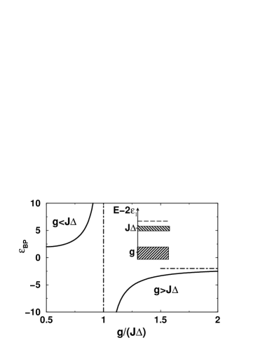
Figure 2: The distance between the energy level of the BP localized next to the defect and the center of the band of extended BP states, $\varepsilon_{BP}=(E_{BP}^{(s)}-E_{BP}^{(0)})/(J/4\Delta)$, vs the scaled defect excess energy $g/J\Delta$. The localized state exists in an infinite chain for $g/J\Delta>1/2$. The vertical and horizontal dot-dashed lines show the asymptotes for $g\to J\Delta$ and $g/J\Delta\to\infty$, respectively. The results refer to the range where the BP and LDP bands are far from each other, compared to the LDP bandwidth $|J|$. These bands are sketched in the inset (the BP band is above the LDP band for $J\Delta/g>1$). The dashed line in the inset shows where the energy level of the localized BP state is located with respect to the bands.

IV Antiresonant decoupling of two-excitation states

The analysis of the preceding section does not apply if the pair binding energy $J\Delta$ is close to the defect excess energy $g$. When $|g-J\Delta|$ is of the order of the LDP bandwidth $|J|$, the BP and LDP states are in resonance, their bands overlap or nearly overlap with each other. One might expect that there would occur mixing of states of these two bands. In other words, a delocalized magnon in the LDP band might be scattered off the excitation on the defect, and as a result they both would move away as a bound pair. However, as we show, such mixing does not happen. In order to simplify notations we will assume in what follows that $g,J,\Delta>0$.

IV.1 A bound pair localized next to the defect

In the resonant region we should reconsider the analysis of the next-to-the-defect bound pair localized on sites $(n_{0}+1,n_{0}+2)$ or $(n_{0}-2,n_{0}-1)$. As $|g-J\Delta|$ decreases, the energy of this pair (26) moves away from the BP band, see Fig. 2. At the same time, the distance between the pair energy and the LDP band $E_{BP}^{(s)}-2\varepsilon_{1}-g$ becomes smaller with decreasing $|g-J\Delta|$ as long as $|J\Delta-g|>|J|/2$. For $|J\Delta-g|\sim J$, the next-to-the-defect pairs are hybridized with LDP’s. The hybridization occurs in first order in the nearest-neighbor coupling constant $J$.

To describe the hybridization, we will seek the solution of the Schrödinger equation (10) in the form of a linear superposition of an LDP state (18) and a pair on the next to the defect sites,

$$a(n,m) = (Ce^{i\theta m}+C^{\prime}e^{-i\theta m})\delta_{n,n_{0}}$$ (27)

$$+ a(n_{0}+1,n_{0}+2)\delta_{n,n_{0}+1}\delta_{m,n_{0}+2}$$

$$+ a(n_{0}-2,n_{0}-1)\delta_{n,n_{0}-2}\delta_{m,n_{0}-1}$$

(we remind that $m>n$). The energy of a state with given $\theta$ can be found from (10) as before by considering $m$ far away from $n_{0}$. It is given by Eq. (19).

The interrelation between the coefficients $C,C^{\prime},a(n_{0}+1,n_{0}+2)$, and $a(n_{0}-2,n_{0}-1)$, as well as the values of $\theta$ should be obtained from the boundary conditions. These conditions follow from the fact that the energy of a pair on sites $(n_{0},n_{0}\pm 1)$ and the energies of the pairs described by Eq.(27) differ by $\sim g\approx J\Delta$, cf. (20). Therefore the pairs on sites $(n_{0},n_{0}\pm 1)$ are decoupled from the states (27), and in the analysis of the LDP’s we can set $a(n_{0},n_{0}\pm 1)=0$. Decoupled also are unbound two-excitation states with no excitation on the defect, i.e., two-magnon states. Therefore $a(n,m)=0$ if simultaneously $m-n>1$ and $(n-n_{0})(m-n_{0})\neq 0$.

From Eq. (10) written for $n=n_{0},m=n_{0}+2$ and $n=n_{0}-2,m=n_{0}$ [with account taken of the relation $a(n,m)=a(m,n+N)$] we obtain

$$a(n_{0}+1,n_{0}+2) = Ce^{i\theta(n_{0}+1)}+C^{\prime}e^{-i\theta(n_{0}+1)},$$ (28)

$$a(n_{0}-2,n_{0}-1) = Ce^{i\theta(n_{0}+N-1)}+C^{\prime}e^{-i\theta(n_{0}+N-1)}.$$

The interrelation between $C$ and $C^{\prime}$ and the equation for $\theta$ follow from Eqs. (27), (28) and (10) written for $n=n_{0}+1,m=n_{0}+2$ and $n=n_{0}-2,m=n_{0}-1$. They have the form

$$C^{\prime}=-\frac{2(J\Delta-g)e^{i\theta}-J}{2(J\Delta-g)e^{-i\theta}-J}Ce^{2i\theta n_{0}},$$ (29)

and

$$\tilde{f}(\theta)=\tilde{f}(-\theta),$$ (30)

$$\tilde{f}(\theta)=e^{i\theta N}\left[2(J\Delta-g)e^{-i\theta}-J\right]^{2}.$$

Equation (30) is an $2N$th order equation for $\exp(i\theta)$. Its analysis is completely analogous to that of Eq. (23). The roots $\theta=0,\pi$ are spurious, and the roots $\theta$ of opposite signs describe one and the same wave function. Therefore Eq. (30) has $N-1$ physically distinct roots $\theta$. Real $\theta$’s correspond to extended states. Complex roots appear for $2|J\Delta-g|>J$. These roots, $\theta_{LDP}^{(s)}$, describe localized states. In the limit of a long chain, $N\to\infty$, the imaginary part of one of them is

$${\rm Im}\,\theta_{LDP}^{(s)}=\ln|2(J\Delta-g)/J|,$$ (31)

whereas the other root has just opposite sign.

The wave function of the localized state is maximal either on sites $(n_{0}+1,n_{0}+2)$ or $(n_{0}-2,n_{0}-1)$ and exponentially decays into the chain. For $J\Delta-g<0$ this decay is accompanied by oscillations, Re $\theta_{LDP}^{(s)}=\pi$. The energy of the localized state is

$$E_{LDP}^{(s)}=2{\varepsilon}_{1}+J\Delta+\frac{(J/2)^{2}}{J\Delta-g}.$$ (32)

The localized state (27), (31) is a “surface-type” state induced by the defect. It is the resonant-region analog of the localized next-to-the-defect state discussed in Section III.B3. The wave function of the latter state (22), (25) was a linear combination of the wave functions of bound pairs. In contrast, the state given by Eqs. (27), (31) is a combination of the wave functions of the bound pair located next to the defect and a localized-delocalized pair.

The evolution of the surface-type state is controlled by the difference between the excess energies of binding two excitations in a pair or localizing one of them on the defect $|J\Delta-g|$. As $|J\Delta-g|$ varies, the state changes in the following way. It first splits off the BP band when $|J\Delta-g|$ becomes less than $g$, see Fig. 2. Its energy moves away from the band of extended BP states with decreasing $|J\Delta-g|$ and the localization length decreases [cf. Eq. (25)]. Well before $|J\Delta-g|$ becomes of order $J$, the state becomes strongly localized on the sites $(n_{0}+1,n_{0}+2)$ or $(n_{0}-2,n_{0}-1)$.

In the region $|J\Delta-g|\sim J$ the localized state becomes stronger hybridized with LDP states than with extended BP states. This hybridization occurs in first order in $J$, via a transition $(n_{0}+1,n_{0}+2)\to(n_{0},n_{0}+2)$ [or $(n_{0}-2,n_{0}-1)\to(n_{0}-2,n_{0})$]. In this region the localization length increases with decreasing $|J\Delta-g|$, cf. Eq. (31). Ultimately, for $|J\Delta-g|=J/2$ the localized surface-type state disappears, as seen in Fig. 3. The evolution of the energy of the localized state with $J\Delta-g$ is shown in Fig. 3.

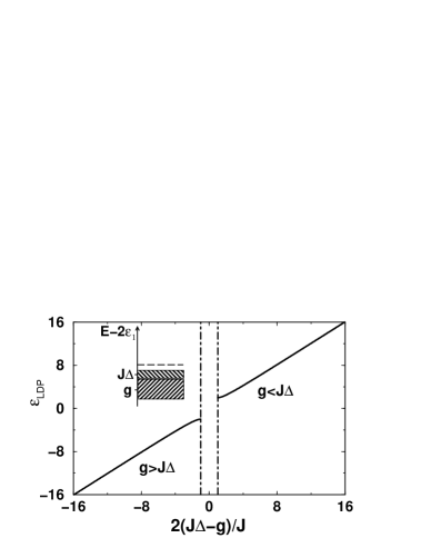
Figure 3: The energy difference between the localized BP state and the LDP band, $\varepsilon_{LDP}=(E_{LDP}^{(s)}-2{\varepsilon}_{1}-g)/(J/2)$, vs the energy mismatch $2(J\Delta-g)/J$. In the region between the dot-dashed lines the BP state is delocalized. The results refer to the case where the BP and LDP bands are close to each other or overlap, as sketched in the inset (the BP band is above the LDP band for $J\Delta>g$). The dashed line in the inset shows where the energy level of the localized BP state is located with respect to the bands.

The crossover from hybridization of the localized surface-type BP state with extended BP states to that with LDP states occurs in the region $|g|\gg|J\Delta-g|\gg|J|$. It is described using a different approach in Ref. us_DS, . We note that the expressions for the energy of the localized states (26) and (32) go over into each other for $|J\Delta-g|\ll|g|$.

IV.2 Decoupling of bound pairs and LDP’s in the resonant region

We are now in a position to consider resonant coupling between extended states of bound pairs and localized-delocalized pairs. To lowest order in $\Delta^{-1}$, a BP on sites $(n,n+1)$ far away from the defect can resonantly hop only to the nearest pair of sites, see Eqs. (III.1), (16). As noted before, the hopping requires an intermediate virtual transition of the BP into a dissociated state, which differs in energy by $J\Delta$.

A different situation occurs for the BP on the sites $(n_{0}+2,n_{0}+3)$ [or $(n_{0}-3,n_{0}-2)$]. Such BP can hop onto the sites $(n_{0}+1,n_{0}+2)$ and $(n_{0}+3,n_{0}+4)$, as described by (16). But in addition, for $|J\Delta-g|\lesssim J$ it can make a transition into the LDP state on sites $(n_{0},n_{0}+3)$ [or $(n_{0}-3,n_{0})$] . Indeed, such state has the energy $\approx 2{\varepsilon}_{1}+g$, which is close to the BP energy $\approx 2{\varepsilon}_{1}+J\Delta$.

The transition $(n_{0}+2,n_{0}+3)\to(n_{0},n_{0}+3)$ goes through the intermediate dissociated state $(n_{0}+1,n_{0}+3)$, which differs in energy by $\approx J\Delta$. It can be taken into account by adding the term $\delta\tilde{H}^{(t)}$ to the BP hopping Hamiltonian (16) for the sites $(n_{0}+2,n_{0}+3)$,

$$\delta\tilde{H}^{(t)}a(n_{0}+2,n_{0}+3)=(J/4\Delta)a(n_{0},n_{0}+3).$$ (33)

Extended BP states are connected to LDP states only through a BP on the sites $(n_{0}+2,n_{0}+3)$. We are now in a position to analyze this connection. From Eqs. (16) and (33), we see that

$$[\tilde{H}^{(t)}+\delta\tilde{H}^{(t)}]a(n_{0}+2,n_{0}+3)=(J/4\Delta)$$

$$\times[a(n_{0},n_{0}+3)+a(n_{0}+1,n_{0}+2)]+A,$$ (34)

where $A$ is a linear combination of the amplitudes $a(n_{0}+2,n_{0}+3)$ and $a(n_{0}+3,n_{0}+4)$.

The sum $a(n_{0},n_{0}+3)+a(n_{0}+1,n_{0}+2)$ in Eq. (IV.2) can be expressed in terms of the LDP wave functions (27). With account taken of the interrelation (29) between the coefficients $C,C^{\prime}$ in Eq. (27), we have

$$a(n_{0}+1,n_{0}+2)+a(n_{0},n_{0}+3)$$

$$\propto C\sin\theta\cos\theta[J\Delta-g-J\cos\theta].$$ (35)

Equations (IV.2), (IV.2) describe the coupling between the BP on the sites $(n_{0}+2,n_{0}+3)$ and the LDP eigenstates with given $\theta$.

An important conclusion can now be drawn regarding the behavior of BP and LDP states in the resonant region. The center of the BP band lies at $2{\varepsilon}_{1}+J\Delta+(J/2\Delta)$ (14), and the BP band is parametrically narrower than the LDP band $2{\varepsilon}_{1}+g+J\cos\theta$ (19). When the BP band is inside the LDP band, this means that, for an appropriate wave number $\theta$ of the LDP magnon, $J\Delta=g+J\cos\theta$, to zeroth order in $\Delta^{-1}$ (this is the approximation used to obtain the LDP dispersion law). It follows from Eqs. (IV.2) and (IV.2) that, for such $J\Delta-g$ and $\theta$ there is no coupling between the LDP and extended BP states.

The above result means that LDP and extended BP states do not experience resonant scattering into each other, even though it is allowed by the energy-conservation law. Such scattering would correspond to the scattering of a magnon off the excitation localized on the defect, with both of them becoming a bound pair that moves away from the defect, or an inverse process.

Physically, the antiresonant decoupling of BP and LDP states is a result of strong mixing of a BP on the sites $(n_{0}+1,n_{0}+2)$ and LDP’s. Because of the mixing, the amplitudes of transitions of extended BP states to the sites $(n_{0}+1,n_{0}+2)$ and $(n_{0},n_{0}+3)$ compensate each other, to lowest order in $\Delta^{-1}$.

To illustrate the antiresonant decoupling we show in Fig. 4 two types of time evolution of excitation pairs. In both cases the initial state of the system was chosen as a pair on the sites $(n_{0}+1,n_{0}+2)$, i.e., $a(n_{0}+1,n_{0}+2)=1$ for $t=0$. The time-dependent Schrödinger equation was then solved with the boundary condition that corresponds to a closed chain.

The solid lines refer to the case of nonoverlapping BP and LDP bands, $|J|\ll|g-J\Delta|$ and $|g|<|J\Delta|/2$. In this case there does not emerge a localized surface-type BP state next to the defect. Therefore an excitation pair placed initially on the sites $(n_{0}+1,n_{0}+2)$ resonantly transforms into extended BP states and propagates through the chain. This propagation is seen from the figure as oscillations of the return probability and the probability to find the BP on another arbitrarily chosen pair of neighboring sites $(n_{0}+2,n_{0}+3)$. The oscillation rate should be small, of the order of the bandwidth $J/\Delta$. This estimate agrees with the numerical data. It is seen that the BP state is not transformed into LDP states. The amplitude of LDP states on sites $(n_{0},m\geq n_{0}+2)$ remains extremely small, as illustrated for $m=n_{0}+2$.

The dotted lines in Fig. 4 show a completely different picture which arises when the BP band is inside the LDP band. In this case an excitation pair placed initially on $(n_{0}+1,n_{0}+2)$ hybridizes with LDP rather than BP states. A transformation of the pair $(n_{0}+1,n_{0}+2)$ into LDP’s with increasing time is clearly seen. The period of oscillations is of the order of the reciprocal bandwidth of the LDP’s $J^{-1}$, it is much shorter than in the previous case. Remarkably, as a consequence of the antiresonance, extended states of bound pairs are not excited to any appreciable extent, as seen from the amplitude of the pair on the sites $(n_{0}+2,n_{0}+3)$.

Figure 4: Time evolution of a two-excitation wave packet in an $XXZ$ chain with a defect; $|a(n,m)|^{2}$ is the occupation of sites $(n,m)$. Initially an excitation pair is placed next to the defect on sites $(n_{0}+1,n_{0}+2)$. The solid and dashed lines refer to the cases where the BP and LDP bands are, respectively, far away from each other ($g=J\Delta/4$) and overlapping ($g=J\Delta$). In the first case a bound pair slowly oscillates between neighboring sites $(n,n+1)$ and does not dissociate [$a(n_{0},n_{0}+2)$ remains very small]. In the case of overlapping bands, the pair at $(n_{0}+1,n_{0}+2)$ is hybridized with LDP’s, but practically does not mix with bound pairs on other sites [$a(n_{0}+2,n_{0}+3)$ remains very small]. The results refer to a ten-site closed chain with $\Delta=10$.

V Conclusions

We have analyzed the dynamics of a disordered spin chain with a strongly anisotropic coupling in a magnetic field. A defect in such a chain can lead to several localized states, depending on the number of excitations. This is a consequence of the interaction between excitations and its interplay with the disorder. We have studied chains with one and two excitations.

The major results refer to the case of two excitations. Here, the physics is determined by the interrelation between the excess on-site energy of the defect $g$ and the anisotropic part of the exchange coupling $J\Delta$. Strong anisotropy leads to binding of excitations into nearest-neighbor pairs that freely propagate in an ideal chain. Because of the defect, BP’s can localize. A simple type of a localized BP is a pair with one of the excitations located on a defect. A less obvious localized state corresponds to a pair localized next to a defect. It reminds of a surface state split off from the band of extended BP states, with the surface being the defect site. We specified the conditions where the localization occurs and found the characteristics of the localized states.

Our most unexpected observation is the antiresonant decoupling of extended BP states from localized-delocalized pairs. The LDP’s are formed by one excitation on the defect site and another in an extended state. The antiresonance occurs for $g\approx J\Delta$, when the BP and LDP bands overlap. It results from destructive quantum interference of the amplitudes of transitions of BP’s into two types of resonant two-excitation states: one is an LDP, and the other is an excitation pair on the sites next to the defect. As a result of the antiresonant decoupling, extended BP’s and LDP’s do not  scatter into each other, even though the scattering is allowed by energy conservation. This means that an excitation localized on the defect does not delocalize as a result of coupling to other excitations.

The occurrence of multiple localized states in the presence of other excitations is important for quantum computing. It shows that, even where the interaction between the qubits is “on” all the time, we may still have well-defined states of individual qubits that can be addressed and controlled. One can prepare entangled localized pairs of excitations, as we discussed in Sec. III B 2, or more complicated entangled excitation complexes. The results of the paper also provide an example of new many-body effects that can be studied using quantum computers with individually controlled qubit transition energies.

Appendix A One excitation

In an infinite spin chain in a magnetic field, the anisotropy of the spin-spin interaction does not affect the spectrum and wave functions of one excitation. The matrix element of the term $\sum_{n}\sigma_{n}^{z}\sigma_{n+1}^{z}$ in the Hamiltonian (1) is just a constant. However, the situation becomes different for a chain of finite length, because the coupling anisotropy can lead to surface states. In the case of two excitations, analogs of surface-type states emerge near defects in an infinite chain, as discussed in Sec. III. Here, for completeness and keeping in mind a reader with the background in quantum computing, we briefly outline the results of the standard analysis of a finite-length spin chain with one excitation.

A.1 Localized surface and defect-induced states in an open chain

The Schrödinger equation for an excitation in an open chain has the form (5), and its solution $a(n)$ to the left and to the right from the defect can be written in the form of a superposition of counterpropagating plane waves, Eq. (6). The relation between the amplitudes of these waves $C^{\prime}_{l,r}$ and $C_{l,r}$ follows from the boundary conditions $a(0)=a(N+1)=0$. By substituting Eq. (6) into Eq. (5) with $n=1$ and $n=N$, we obtain

$$C^{\prime}_{l}=-DC_{l},\quad C^{\prime}_{r}=-D^{-1}e^{2i\theta(N+1)}C_{r},$$ (36)

$$D=[1-\Delta\exp(i\theta)]/[1-\Delta\exp(-i\theta)].$$

The relations between $C^{\prime}_{l,r}$, $C_{l,r}$, and the amplitude of the wave function on the defect site $a(n_{0})$ follow from Eqs. (5) and (6) for $n=n_{0}\pm 1$,

$$a(n_{0}) =C_{l}e^{i\theta n_{0}}\left[1-De^{-2i\theta n_{0}}\right]$$ (37)

$$=C_{r}e^{i\theta n_{0}}\left[1-D^{-1}e^{2i\theta(N+1-n_{0})}\right].$$

With (36) and (37), all coefficients in the wave function (6) are expressed in terms of one number, $a(n_{0})$. It can be obtained from normalization.

In a finite chain, the values of $\theta$ are quantized. They can be found from Eq. (5) with $n=n_{0}$. With account taken of (37), this equation can be written as

$$f_{N}(\theta)-D^{2}f_{N}(-\theta)=-(ig/J\sin\theta)\qquad\qquad\qquad$$

$$\times[f_{N}(\theta)+D^{2}f_{N}(-\theta)-2D\cos\theta(N-2n_{0}+1)],$$ (38)

where

$$f_{N}(\theta)=\exp[i\theta(N+1)].$$ (39)

The analysis of the roots of Eq. (A.1) is standard. This is a $2(N+1)$-order equation for $\exp(i\theta)$, but its solutions for $\theta$ come in pairs $\theta$ and $-\theta$. Each pair gives one wave function, as seen from Eq. (6). In addition, Eq. (A.1) has roots $\theta=0,\pi$; they are spurious (unless $|\Delta|=1$ and $g=0$) and appear as a result of algebraic transformations. Therefore Eq. (A.1) has $N$ physically distinct roots, as expected for a chain of $N$ spins. We note that, for $g=0$ the position of the impurity $n_{0}$ drops out from Eq. (A.1), and then the equation goes over into the result for an ideal chain.

Solutions of Eq. (A.1) with real $\theta$ correspond, in the case of a long chain, to delocalized magnon-type excitations propagating in the chain. Their bandwidth is $2|J|$.

Along with delocalized states, Eq. (A.1) describes also localized states with complex $\theta$. Complex roots of Eq. (A.1) can be found for a long chain, where $|{\rm Im}\,\theta|(N-n_{0}),\,|{\rm Im}\,\theta|n_{0}\gg 1$. They describe surface states, which are localized on the chain boundaries, and a state localized on the defect. The localization length of the states is given by $|1/{\rm Im}\,\theta|$.

The surface states arise only for the anisotropy parameter $|\Delta|>1$. The corresponding values of $\theta$ are

$$\theta_{s}=\pm i\ln|\Delta|+\pi\Theta(-\Delta).$$ (40)

Here, the signs $+$ and $-$ refer to the states localized on the left and right boundaries, respectively, and $\Theta(x)$ is the step function.

From Eq. (8), the energy of the surface state is

$$E_{s}={\varepsilon}_{1}+J(\Delta^{2}+1)/2\Delta$$ (41)

It lies outside the energy band of delocalized excitations. We note that, for $\Delta>1$ the surface states decay monotonically with the distance from the boundary (Re $\theta=0$). For sufficiently large negative $\Delta$, on the other hand, the decay of the wave function is accompanied by oscillations, and $a(n)$ changes sign from site to site.

A defect in a long chain gives rise to a localized one-spin excitation for an arbitrary excess energy $g$ Economou . The amplitude $a(n)$ decays away from the defect as

$$a(n)=a(n_{0})\exp(i\theta_{d}|n-n_{0}|),$$ (42)

$$\theta_{d}=i\sinh^{-1}(|g/J|)+\pi\Theta(-g/J).$$

The energy of the localized state is

$$E_{d}=\varepsilon_{1}+(g^{2}+J^{2})^{1/2}{\rm sgn}\,g.$$ (43)

For small $|g/J|$, we have Im $\theta_{d}\approx|g/J|$, i.e., the reciprocal localization length is simply proportional to the defect excess energy $|g|$. In the opposite case of large $|g/J|$ we have Im $\theta_{d}=\ln|2g/J|$. In this case the amplitude of the localized state rapidly falls off with the distance from the defect, $a(n)\propto(2|g/J|)^{-|n-n_{0}|}$.

If the localization length is comparable to the chain length, the notion of localization is not well defined. However, when discussing numerical results, one can formally call a state localized if its wave function exponentially decays away from the defect and is described by a solution of Eq. (A.1) with complex $\theta$. This is equivalent to the statement that the state energy $E_{d}$ lies outside the band of magnons in the infinite chain. In an open finite chain such localized state may emerge provided the localization length is smaller than the distance from the defect to the boundaries. This means that the defect excess energy $|g|$ should exceed a minimal value that depends on the size of the chain. The comparison of Eq. (42) with the numerical solutions of the full equation (A.1) for a finite chain is shown in Fig. 5.

Figure 5: The reciprocal localization length Im $\theta_{d}$ for an infinite chain [Eq. (42)] as a function of the defect excess energy $g$ for $J=1$ (solid line). Also shown are the results for an open chain with the number of sites $N=6$ and 12 and $n_{0}=N/2$ (stars and crosses, respectively) and a closed chain with 6 and 12 sites (circles and squares, respectively). They are obtained from Eq. (A.1) with $\Delta=10$ and from Eq. (46). In an open chain, solutions with nonzero Im $\theta_{d}$ emerge starting with a certain $|g/J|>|g/J|_{\min}$. In a closed chain with even $N$ there is no threshold in $|g/J|$ for the onset of states with Im $\theta_{d}\neq 0$.

A.2 One-excitation states in a closed chain

As pointed out in Sec. II, for a closed chain the solution of the Schrödinger equation can be also sought in the form of counterpropagating waves with different amplitudes, Eq. (7). Clearly, the phases $\theta$ and $-\theta$ describe one and the same wave function. The one-excitation energy $E_{1}$ is given by Eq. (8).

The interrelation between the amplitudes of the waves $C,C^{\prime}$ in Eq. (7) and the amplitude of the wave function on the defect site $a(n_{0})$ can be obtained from Eq. (5) with $n=n_{0}\pm 1$. This equation has two solutions,

$$e^{i\theta N}=1,\quad a(n_{0})=Ce^{i\theta n_{0}}+C^{\prime}e^{-i\theta n_{0}}$$ (44)

and

$$a(n_{0}) = Ce^{i\theta n_{0}}\left(1+e^{i\theta N}\right)$$

$$= C^{\prime}e^{-i\theta n_{0}}\left(1+e^{-i\theta N}\right)\quad[\exp(i\theta N)\neq 1].$$

In order to fully determine the wave function $a(n)$ (7), Eqs. (44), (A.2) should be substituted into the Schrödinger equation (5) for $n=n_{0}$.

Equations (5) and (44) can be satisfied provided that either $g=0$, which means that there is no defect, or $a(n_{0})=0$. The first condition describes excitations in an ideal closed chain and is not interesting for the present paper. The condition $a(n_{0})=0$ corresponds to the wave function $a(n)\propto\sin\theta(n-n_{0})$, which has a simple physical meaning. It is a standing wave in an ideal chain with a node at the location of a defect. Because of the node, the corresponding state “does not know” about the defect, and therefore it is exactly the same as in an ideal chain.

In the presence of a defect, the solutions of Eq. (44) in the range of interest $0<\theta<\pi$ are $\theta=2\pi k/N$ with $k=1,2,\ldots,(N-1)/2$ for odd $N$, or $k=1,2,\ldots,N/2-1$ for even $N$.

The equation for $\theta$ that follows from Eqs. (5) and (A.2) has the form

$$\exp(i\theta N)-1=-\frac{ig}{J\sin\theta}[\exp(i\theta N)+1].$$ (46)

For $g\neq 0$ this equation has either $(N+1)/2$ (for odd $N$) or $N/2+1$ (for even $N$) solutions for $\pm\theta$. Therefore the total number of solutions for $\theta$ that follow from Eqs. (44) and (46) is $N$, as expected.

By rewriting Eq. (46) as $\tan(\theta N/2)=-(g/J\sin\theta)$ and plotting the left- and right-hand sides as functions of $\theta$ (cf. Ref. Economou, ), one can see that all physically distinct roots of this equation but one are real and lie in the interval $0<\theta<\pi$ [except for one case, see below]. Such solutions describe delocalized states with sinusoidal wave functions.

The complex root of Eq. (46), $\theta=\theta_{d}$, describes a state localized on the defect. For a long chain, Im $\theta_{d}N\gg 1$, the solution has the form (42), as expected. An interesting situation occurs for a shorter chain. If $N$ is even or if $g/J>0$, a localized solution with complex $\theta_{d}$ emerges for any defect excess energy $g$. Thresholdless localization does not happen in an open chain. In a closed chain, it arises because there is no reflection from boundaries. For small positive $g/J$ one obtains the complex solution of Eq. (46) in the form $\theta_{d}\approx i(2g/NJ)^{1/2}$. The square-root dependence of Im $\theta_{d}$ on $g$ is seen from Fig. 5.

Equation (46) has a complex solution also for even $N$ and small negative $g/J$. In this case $\theta_{d}\approx i(-2g/NJ)^{1/2}+\pi$, i.e., the decay of the wave function $a(n)$ is accompanied by sign flips, $a(n+1)/a(n)<0$. Such oscillations cannot be reconciled with the periodicity condition for odd $N$. Therefore, for odd $N$ and negative $g/J$ a decaying solution arises only when $-g/J$ exceeds a threshold value. One can show from Eq. (46) that this value is $|g/J|_{\min}=2/N$, which has also been confirmed numerically.

References

- (1) M.A. Nielsen and I.L. Chuang, Quantum Computation and Quantum Information (Cambridge University Press, Cambridge, 2000).
- (2) Y. Makhlin, G. Schön, and A. Shnirman, Rev. Mod. Phys. 73, 357 (2001).
- (3) D. Vion, A. Aassime, A. Cottet, P. Joyez, H. Pothier, C. Urbina, D. Esteve, and M.H. Devoret, Science 296, 886 (2002); Y. Yu, S.Y. Han, X. Chu, S.I. Chu, and Z. Wang, ibid 296, 889 (2002); Y.A. Pashkin, T. Yamamoto, O. Astafiev, Y. Nakamura, D.V. Averin, and J.S. Tsai, Nature (London) 421, 823 (2002); A.J. Berkley, H. Xu, R.C. Ramos, M.A. Gubrud, F.W. Trauch, P.R. Johnson, J.R. Anderson, A.J. Dragt, C.J. Lobb, and F.C. Wellstood, Science 300, 1548 (2003).
- (4) P.M. Platzman and M.I. Dykman, Science 284, 1967 (1999); M.I. Dykman and P.M. Platzman, Fortschr. Phys. 48, 9 (2000); M.I. Dykman, P.M. Platzman, and P. Seddighrad, Phys. Rev. B 67, 155402 (2003).
- (5) I.L. Chuang, L.M.K. Vandersypen, X. Zhou, D.B. Leung, and S. Lloyd, Nature (London) 393, 143 (1998); L.M.K. Vandersypen, M. Steffen, G. Breyta, C.S. Yannoni, M.H. Sherwood, and I.L. Chuang, ibid 414, 883 (2001).
- (6) T.D. Ladd, J.R. Goldman, F. Yamaguchi, Y. Yamamoto, E. Abe, and K.M. Itoh, Phys. Rev. Lett. 89, 017901 (2002).
- (7) D.G. Cory, R. Laflamme, E. Knill, L. Viola, T.F. Havel, N. Bouland, G. Boutis, E. Fortunato, S. Lloyd, R. Martinez, C. Negrevergne, M. Pravia, Y. Sharf, G. Teklemariam, Y.S. Weinstein, and W.H. Zurek, Fortschr. Phys. 48, 875 (2000).
- (8) P. Chen, C. Piermarocchi, and L.J. Sham, Phys. Rev. Lett. 87, 067401 (2001); X. Li, Y. Wu, D.G. Steel, D. Gammon, T.H. Stievater, D.S. Katzer, D. Park, L.J. Sham, and C. Piermarocchi, Science 301, 809 (2003).
- (9) D. DeMille, Phys. Rev. Lett. 88, 067901 (2002).
- (10) P.G. Silvestrov, H. Schomerus, and C.W.J. Beenakker, Phys. Rev. Lett. 86, 5192 (2001);
- (11) W.M. Kaminsky and S. Lloyd quant-ph/0211152.
- (12) H.A. Bethe, Z. Phys. 71, 205 (1931); C.N. Yang and C.P. Yang, Phys. Rev. 150, 321, 327 (1966).
- (13) F.C. Alcaraz, M.N. Barber, M.T. Batchelor, R.J. Baxter and G.R.W. Quispel, J. Phys. A. 20, 6397 (1987).
- (14) P. Schmitteckert, P. Schwab, and U. Eckern, Europhys. Lett. 30, 543 (1995); H.-P. Eckle, A. Punnoose, and R.A. Römer, Europhys. Lett. 39, 293 (1997); A. Zvyagin, J. Phys. A 34, R21 (2001).
- (15) B. Georgeot and D.L. Shepelyansky, Phys. Rev. E 62, 3504, 6366 (2000).
- (16) G.P. Berman, F. Borgonovi, F.M. Izrailev, and V.I. Tsifrinovich, Phys. Rev. E 64, 056226 (2001); ibid 65, 015204 (2002).
- (17) V.V. Flambaum, Aust. J. Phys. 53, 489 (2000); J. Emerson, Y.S. Weinstein, S. Lloyd, and D.G. Cory, Phys. Rev. Lett. 89, 284102 (2002).
- (18) G.F. Koster and J.C. Slater, Phys. Rev. 95, 1167 (1954); E.N. Economou, Green’s function in quantum physics, (Springer-Verlag, Berlin, New York, 1979).
- (19) J.M. Goodkind and S. Pilla, Quantum Information and Computation 1, 108 (2001).
- (20) M.I. Dykman and L.F. Santos, J. Phys. A 36, L561 (2003).