Macroscopic Quantum Resonance of Coupled Flux Qubits;
 A Quantum Computation Scheme

Abstract

We show that a superconducting circuit containing two loops, when treated with Macroscopic Quantum Coherence (MQC) theory, constitutes a complete two-bit quantum computer. The manipulation of the system is easily implemented with alternating magnetic fields. A universal set of quantum gates is deemed available by means of all unitary single bit operations and a controlled-not (cnot) sequence. We use multi-dimensional MQC theory and time-dependent first order perturbation theory to analyze the model. Our calculations show that a two qubit arrangement, each having a diameter of 200nm, operating in the flux regime can be operated with a static magnetic field of $\sim 0.1$T, and an alternating dynamic magnetic field of amplitude $\sim 1$ Gauss and frequency $\sim 10$Hz. The operational time $\tau_{op}$ is estimated to be $\sim 10$ns.

I INTRODUCTION

In the last few decades there has been broad interest in hope to design and construct a practical quantum computer. The, so to speak, machines will enable us to reach a domain of knowledge that was, up to now, considered unreachable or beyond human capabilities. They will allow us to perform calculations of enormous amount in a rapid and effective manner. Factoring large numbers, teleporting large amounts of information, and simulation of the real world, will enter our immediate reach and are destined to dramatically changes our lives.

The core role of quantum computers are played by quantum bits, qubits. Many ideas have been raised for practical qubit realization: cavity quantum electrodynamics, ion traps and nuclear spins. Also, superconducting circuits of Josephson junctions have been proposed and experimental research is being pursued. In this paper we will show a possibility to implement a quantum computation scheme on a coupled flux qubit system. In the rest of this introduction we will give a brief description of the idea of quantum computation, and also, an outline of the macroscopic quantum coherence theory (MQC), with which we treat our system.

I.1 Quantum computation

Quantum computers have attracted a lot of attention and an abundance of work has been established. But here, we will concentrate on only the main aspects of quantum computers. Least requirements for a quantum computer are that the system must retain certain properties:

1. Ability to represent quantum information, meaning that a quantum bit must be able to represent not only two classical values $|0\rangle$ and $|1\rangle$, but also a superposition of these two states, namely $\alpha|0\rangle+\beta|1\rangle$, where $\alpha$ and $\beta$ are c-numbers.

2. Have a universal family of unitary transformations. Universal, here represents that the Hamiltonian of the system is capable of controlling the system state arbitrarily. In other words one must be able to reversibly transform any given state into another state of choice. The reversibility is a quantum mechanical requirement. DiVincenzo DiVincenzo (1995) showed that a controlled-not (cnot) and single qubit gates were universal for any $n$-qubit system.

3. Have a preparable initial state. This is an obvious demand, since the initial state of the system is the input. However there is no necessity for capability to provide an arbitrary initial state, since the above requirement suffices to transform a particular initial state into the desired input.

4. Have a means of measurement. One must be able to measure the probability amplitude of the final state, i.e. the output. Measurement of the system state is often the result of the qubit’s coupling to a classical system, commonly the environment. This process is equivalent to a projection of the superposed quantum state of the qubits. Although each measurement outcome is generically random, by controlling ensembles of quantum computers one is capable of determining the output state. In fact, a measurement does destroy the superposition and acts randomly, so one must be sensitive to unwanted measurement which is a cause of decoherence.

All quantum computers must satisfy the above four requirements, plus many others for optimal and efficient computing. A qubit, due to its quantum nature, suffers from decoherence, where the coherent superposition of quantum states is destroyed by noise. This is the most influential obstacle in creating a practical quantum computer. Extracting all noise sources from the system is definitely impossible, but if we could perform our operation before the system loses its coherence then we could obtain our output with relatively high fidelity. Provided, a strong requirement for an efficient quantum computer would be for the ‘quality factor’, $\tau_{d}/\tau_{op}\gtrsim 10^{4}$ Orlando et al. (1999). $\tau_{op}$ is the time necessary for a single operation, and $\tau_{d}$ is the decoherence time: the time length that the system can maintain its coherence.

The coupling of qubits play an important role in quantum computation. To create large scale accurate quantum computers, there must exist an efficient method of coupling selected qubits, and to apply transformations upon the coupled qubits. Although coupling within the system is permissible, often the system couples to the environment thus resulting in considerable noise. This is an important point.

I.2 The quantum mechanics of flux qubits

In our research, we have chosen superconducting circuits as our qubit arrangement. The advantages are that: they are relatively easy to fabricate, they can be measured easily, and large arrays can be effectively implemented. Many of these characteristics are results due to the fact of the flux qubit being a macroscopic device.

However, because of its macroscopic nature an obvious question rises: Does it behave purely quantum mechanically? In other words, can the device be put in a superposition of two distinct states? The answer to this question is provided by Macroscopic Quantum Tunneling or Macroscopic Quantum Coherence (MQT/MQC) theory. This field of study concerning superconducting loops was first developed theoretically by Ivanchenko et. al. Ivanchenko and Zilberman (1968), and Caldeira and Leggett Caldeira and Leggett (1983). Experiments that followed Martinis et al. (1987); R.Rouse et al. (1995) have confirmed so far that the magnitude of magnetic flux piercing a superconducting loop, when seen as a canonical variable, does obey the rules of quantum mechanics.

We distinguish each state of the system by the direction of electric current, so each state is macroscopically distinct. Here, we step out of fundamental quantum mechanics and see that a macroscopic matter can take a state not definitely $|a\rangle$ nor $|b\rangle$, but $\alpha|a\rangle+\beta|b\rangle$. This occurs paradoxical to the sane mind, and has been a discipline of long discussion Einstein et al. (1935): can the cat be dead and alive? Although it is a fundamental aspect, we will not indulge ourselves with a discussion of the EPR paradox here.

Furthermore, theory Chakravarty and Kivelson (1983, 1985); Averin et al. (2000) and experiments Friedman et al. (2000); Han et al. (2000) have shown that transition between these macroscopically distinct states can be induced by photons or dynamically alternating magnetic fields.

Consequently, the tools of the trade for quantum computers can be provided with superconducting circuits. However there still has not been found proof to whether MQT/MQC theory can be applied to systems with more than one degree of freedom, each being a macroscopic value. Experiments Sharifi et al. (1988); S.Han et al. (1989) have shown evidence that MQT does occur in the thermal regime, but also indicate that the interaction between degrees of freedom, resulting in a suppression of escape rates, cannot be ignored. In a recent experiment Li et al. (2002), the quantum regime MQT theory seems to agree well with the behavior of a system with more than one degree of freedom.

II DOUBLE QUBIT SYSTEM

II.1 Description of model

Figure 1: The double qubit model. The crosses represent Josephson junctions, and the lines superconducting nodes. Each loop represents a qubit, and tunneling current circulates the circuit.

In this paper, we have taken a superconducting circuit as is shown in Fig. 1. The model consists of six Josephson junctions and five superconducting nodes. The two loops of the circuit correspond to the two qubits.

II.2 Static properties

We assume that the temperature can be lowered well below $\Delta_{G}/k_{B}$, where $\Delta_{G}$ is the gap energy of the superconductor and $k_{B}$ the Boltzmann constant. Allowing this assumption we proceed with our analysis on the basis that each node is in a coherent state, i.e. maintaining a single value order parameter throughout the node.

We apply a uniform static magnetic field perpendicular to the plane the circuit rests in. By taking the phase difference of each junction $\gamma_{i}$ as our macroscopic variable, from Josephson’s Law, the tunnel current flowing through each junction becomes,

$$I_{k}=I_{c}^{\small{k}}\sin\gamma_{k},$$ (1)

where, $I_{c}^{\small{k}}$ is the critical current of the $k$-th junction. From the single valuedness of the order parameter, we see that the $\gamma$s must always satisfy the conditions,

$$\gamma_{1}+\gamma_{2}-\gamma_{3} = 2\pi f,$$ (2a)

$$-\gamma_{2}+\gamma_{4}+\gamma_{5}-\gamma_{6} = 2\pi f,$$ (2b)

where $f$ represents the magnetic flux through the loops, measured in units of flux quanta $\Phi_{0}$, and is often referred to as the frustration index. The junction energy of this system can be seen to be

$$\mathcal{U}(\vec{\gamma}) = \mathcal{U}_{J}(\vec{\gamma})+\mathcal{U}_{mag}(\vec{\gamma})$$ (3)

$$= \sum_{i=1}^{6}E_{i}\left(1-\cos\gamma_{i}\right)+\mathcal{U}_{mag}(\vec{\gamma}),$$

where $E_{i}$ represents the junction of energy of the $i$-th junction, and $\mathcal{U}_{mag}(\vec{\gamma})$ is the magnetic energy of the system. This is an analogous extension of the washboard model to multi-dimensions. According to MQT/MQC theory, the whole system can be regarded as a free particle with position $\vec{\gamma}$ moving within a potential $\mathcal{U}$.

For the kinetic energy of the system we take in the electrostatic energy of the junctions. According to Josephson’s law, in a non-zero voltage state, the voltage across the junction can be expressed as

$$V_{i}=\frac{\hbar}{2e}\dot{\gamma_{i}}.$$ (4)

Each junction has a capacitance designated as $C_{i}$. Provided, the electrostatic energy of the $i$-th junction becomes

$$\mathcal{T}_{i}(\dot{\gamma_{i}})=\frac{1}{2}C_{i}V_{i}^{2}=\frac{C_{i}}{2}\left(\frac{\hbar}{2e}\right)^{2}\dot{\gamma_{i}}^{2}$$ (5)

, and the total electrostatic energy is simply the sum,

$$\mathcal{T}(\dot{\vec{\gamma}})=\sum^{6}_{i=1}\mathcal{T}_{i}(\dot{\gamma_{i}})$$ (6)

. In a straightforward manner, we have the Lagrangian:

$$\mathcal{L}\left(\dot{\vec{\gamma}},\vec{\gamma}\right) = \mathcal{T}(\dot{\vec{\gamma}})-\mathcal{U}(\vec{\gamma}).$$ (7)

Here, we apply the constraints Eq.(2) by letting

$$\dot{\gamma_{1}}+\dot{\gamma_{2}}-\dot{\gamma_{3}} = 0,$$ (8a)

$$-\dot{\gamma_{2}}+\dot{\gamma_{4}}+\dot{\gamma_{5}}-\dot{\gamma_{6}} = 0,$$ (8b)

and the Lagrangian then becomes

$$\mathcal{L} = \frac{1}{2}\dot{\vec{\gamma}}^{\prime t}\mathrm{C}\dot{\vec{\gamma}}^{\prime}-\mathcal{U}\left(\gamma^{\prime}\right)$$ (9)

where, $\vec{\gamma}^{\prime}=\left(\gamma_{2},\gamma_{3},\gamma_{4},\gamma_{5}\right)$, and $\mathrm{C}$ is the coefficient matrix of the bilinear form for the charging energy. Therefore the conjugate momentum of $\vec{\gamma}$ becomes

$$\vec{p}=\frac{\partial\mathcal{L}}{\partial\dot{\vec{\gamma}}^{\prime}}=\mathrm{C}\dot{\vec{\gamma}}^{\prime},$$ (10)

where $\mathrm{C}$ is a tensor of rank two. By applying a Legendre transformation, we obtain the Hamiltonian of the system,

$$\mathcal{H} = \vec{p}^{\hskip 2.84526ptt}\dot{\vec{\gamma}}^{\prime}-\mathcal{L}$$ (11)

$$= \frac{1}{2}\vec{p}^{\hskip 2.84526ptt}\mathrm{C}^{-1}\vec{p}^{\hskip 2.84526pt}+\mathcal{U}\left(\vec{\gamma}^{\prime}\right).$$

Notice that here, $\mathrm{C}$ is a tensor relevant to the inverse mass of a certain “particle”. From now on the system under consideration will be, given the theoretical analogy, referred to as the “particle” moving within a potential $\mathcal{U}\left(\vec{\gamma}^{\prime}\right)$

For a quantum mechanical treatment, one now introduces the fundamental replacement,

$$\hat{p}=-i\hbar\frac{\partial}{\partial\gamma}.$$ (12)

After this replacement the quantum mechanical Hamiltonian can be written as,

$$\mathcal{H} = \frac{1}{2}\vec{p}^{\hskip 2.84526ptt}\mathrm{C}^{-1}\vec{p}^{\hskip 2.84526pt}$$ (13)

$$+E_{1}\{1-\cos(-\gamma_{2}+\gamma_{3}+2\pi f)\}+\sum_{i=2}^{5}E_{i}\left(1-\cos\gamma_{i}\right)$$

$$+E_{6}\{1-\cos(-\gamma_{2}+\gamma_{4}+\gamma_{5}-2\pi f)\}$$

$$\equiv \tilde{\mathcal{T}}(\gamma_{2},\cdots,\gamma_{5},f)+\tilde{\mathcal{U}}(\gamma_{2},\cdots,\gamma_{5},f)$$ (14)

To determine the motion of the “particle”, we study the reduced potential term $\tilde{\mathcal{U}}(\gamma_{2},\cdots,\gamma_{4},f)$. In Fig. 2, we show $\tilde{\mathcal{U}}(\gamma_{2},\cdots,\gamma_{5},f)$ at $f=0.5$, projected on to a two dimensional space. It is merely a guide to the eye, but clearly shows four metastable states, where the “particle” will be able to rest.

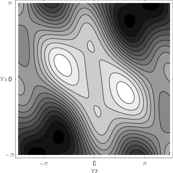
Figure 2: The reduced potential $\tilde{\mathcal{U}}(\gamma_{2},\cdots,\gamma_{5},f=0.5)$ projected on to a two dimensional space, in which the four local minimums (light-colored sections) of $\tilde{\mathcal{U}}$ exists. Each local minimum corresponds to a distinct macroscopic state of the system, from the upper most in clockwise order: $|0\rangle$$|0\rangle$, $|1\rangle$$|0\rangle$, $|1\rangle$$|1\rangle$, $|0\rangle$$|1\rangle$.

We used a simple conjugate gradient method to determine the local minimums of $\tilde{\mathcal{U}}$. The energy level of each metastable state can be seen in Fig. 3. One can see that, even after a slight shift in $f$, as long as $0.5-f_{c}\leq f\leq 0.5+f_{c}$, the system retains its four metastable states. Calculation shows that $f_{c}\simeq 0.05$. Each of the four states differ in current direction, and the behavior is symbolically expressed in Fig. 4, and the numerical data is listed in Table. 1.

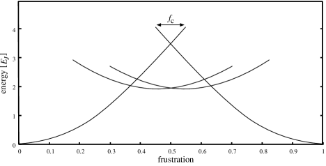
Figure 3: The energy levels of metastable states versus the frustration index $f$. There exits four metastable states when $0.5-f_{c}\leq f\leq 0.5+f_{c}$, $f_{c}\simeq 0.05$. All Josephson junction energies are set equal to $E_{J}$.

Figure 4: Symbolic representation of the distinct states. The arrows indicate the direction of the tunneling current.

Table 1: Values of the phase difference at each junction for each state, in radians. The symbol within the parentheses represent the tunnel current direction (through Eq.(1)), in accordance with Fig. 1.

	$|0\rangle$$|0\rangle$	$|0\rangle$$|1\rangle$	$|1\rangle$$|0\rangle$	$|1\rangle$$|1\rangle$
Junction 1	-1.52 ($\leftarrow$)	-0.57 ($\leftarrow$)	0.57 ($\to$)	1.51 ($\to$)
Junction 2	0.0 (-)	4.28 ($\downarrow$)	2.01 ($\uparrow$)	0.0(-)
Junction 3	1.51($\to$)	0.57 ($\to$)	-0.57 ($\leftarrow$)	-1.52 ($\leftarrow$)
Junction 4	-1.08 ($\leftarrow$)	0.38 ($\to$)	-0.38 ($\leftarrow$)	1.08 ($\to$)
Junction 5	-1.08 ($\downarrow$)	0.38 ($\uparrow$)	-0.38 ($\downarrow$)	1.08 ($\uparrow$)
Junction 6	1.08 ($\to$)	-0.38 ($\leftarrow$)	0.38 ($\to$)	-1.08 ($\leftarrow$)

Flux qubits represent each of the two states, $|0\rangle$ and $|1\rangle$ by current direction. $|0\rangle$ corresponding to clockwise current in the loop and $|1\rangle$, counter-clockwise. The left and right loops will suffice to represent two distinct states, and we can see the system is capable of providing four quantum states, $|0\rangle|0\rangle,|0\rangle|1\rangle,|1\rangle|0\rangle,|1\rangle|1\rangle$, which are the basis of a two-bit quantum computer.

The important aspect of the circuit is that it contains many parameters that can be selected by the operator. Changes in junction energies $E_{i}$, and the junction capacitance $C_{i}$, varies the energy level of the metastable states. Hence $f_{c}$ varies along, and for some parameter settings, the system loses its four state configuration. But by adjusting the $E_{i}$s and the $C_{i}$s, the operator is capable of preparing optimum configuration, in accordance with the experimental factors.

II.3 Manipulation of qubits

The dynamical control of the qubits’ state, is essential to effective quantum computation. We now introduce a scheme for manipulating the qubits in a simple yet efficient manner.

We set $f$ slightly away from $0.5$, yet within the four-state regime. By this, we see from Fig. 3 that the four states each correspond to local potential minimum with different energies. We approximate the bottom of each local minimum of $\tilde{\mathcal{U}}$ with a multi-dimensional harmonic oscillator. Hence the “particle” wave function $|i\rangle|j\rangle$ will practically be a Gaussian wave packet standing at the corresponding minimum. Here and on, notation $|i,j\rangle$ may be used for $|i\rangle$$|j\rangle$, and $\epsilon_{ij}$ for its ground state energy. We induce transitions between states by applying a time-dependent perturbation. Physically, a time dependent magnetic field, oscillating at certain frequencies, applied perpendicular to the circuit will result as a perturbation fulfilling our need. We assume that the particle state ket $|\psi\rangle$ will always stay within the Hilbert space spanned by $|i,j\rangle$ ($i,j=1,2$), and with this as base kets , the Hamiltonian (13) plus a time dependent perturbation can be represented as,

$$\mathcal{H} \equiv \mathcal{H}_{0}+\mathcal{V}\cos\left(\omega t+\varphi\right)$$ (25)

$$\doteq \left(\vspace{2mm}\begin{array}[]{cccc}\vspace{2mm}\epsilon_{00}&\Delta^{01}_{00}&\Delta^{10}_{00}&0\\ \vspace{2mm}\Delta^{01}_{00}&\epsilon_{01}&0&\Delta^{11}_{01}\\ \vspace{2mm}\Delta^{10}_{00}&0&\epsilon_{10}&\Delta^{11}_{10}\\ 0&\Delta^{11}_{01}&\Delta^{11}_{10}&\epsilon_{11}\end{array}\right)+\left(\begin{array}[]{cccc}\begin{array}[]{cc}\vspace{2mm}\mathcal{V}_{00}&\\ \vspace{2mm}\hfil&\mathcal{V}_{01}\end{array}&0\\ 0&\begin{array}[]{cc}\vspace{2mm}\mathcal{V}_{10}&\\ \vspace{2mm}\hfil&\mathcal{V}_{11}\end{array}\end{array}\right)\cos\left(\omega t+\varphi\right).$$

$\Delta_{ij}^{kl}$ represents the tunneling probability for transition $|i,j\rangle\longleftrightarrow|k,l\rangle$. We have used, pfrom the Hermiticity of the Hamiltonian, $\Delta^{kl}_{ij}=\Delta^{ij}_{kl}$. Notice that we have introduced an approximation that, tunneling: $|0,0\rangle\longleftrightarrow|1,1\rangle$ and $|1,0\rangle\longleftrightarrow|0,1\rangle$ are disallowed. Though this may lack rigor, by looking at Fig. 2, it should be clearly acceptable. The perturbation terms,

$$\mathcal{V}_{ij} = \mathcal{V}_{ij}^{M}+\mathcal{V}_{ij}^{J}$$ (26)

$$\equiv \left(\sum_{k=1,2}\frac{\phi^{k}_{ij}}{L_{k}}\right)\delta\phi_{ext}+2\pi\left\{\right.-E_{1}\sin\left(-\gamma_{2}^{ij}+\gamma_{3}^{ij}+2\pi f\right)$$

$$\hskip 99.58464pt+\left.E_{6}\sin\left(-\gamma_{2}^{ij}+\gamma_{4}^{ij}+\gamma_{5}^{ij}-2\pi f\right)\right\}\delta f,$$

where, $L_{k}$ is the self-inductance of the $k$-th qubit, $\delta\phi_{ext}$ the amplitude of the alternating magnetic field, $\delta f=\delta\phi_{ext}/\mathrm{\Phi_{0}}$, and $\phi_{ij}^{k}$ and $\gamma_{k}^{ij}$ are the magnetic flux piercing the $k$-th qubit and the phase value, respectively, while the system is in state $|\psi_{ij}\rangle$. $\mathcal{V}_{ij}^{M}$ resembles the magnetic response of the system and $\mathcal{V}_{ij}^{J}$ is the response of the Josephson junctions to the magnetic perturbation.

Under the approximation that tunneling probability is small, we expand the energy eigen kets in powers of the $\Delta$s. The zeroth order term of the Hamiltonian (25) contains no off diagonal elements, and therefore no tunneling occurs. By taking in up to first order terms, the eigen energy functions, up to a normalization factor, become

$$|\psi_{00}\rangle = \left(2\epsilon_{00}-\epsilon_{01}-\epsilon_{10}\right)|00\rangle+\Delta^{10}_{00}|10\rangle+\Delta^{01}_{00}|01\rangle,$$ (27a)

$$|\psi_{01}\rangle = \left(2\epsilon_{01}-\epsilon_{00}-\epsilon_{11}\right)|01\rangle+\Delta^{00}_{01}|00\rangle+\Delta^{11}_{01}|11\rangle,$$ (27b)

$$|\psi_{10}\rangle = \left(2\epsilon_{10}-\epsilon_{00}-\epsilon_{11}\right)|10\rangle+\Delta^{00}_{10}|00\rangle+\Delta^{11}_{10}|11\rangle,$$ (27c)

$$|\psi_{11}\rangle = \left(2\epsilon_{11}-\epsilon_{01}-\epsilon_{10}\right)|11\rangle+\Delta^{01}_{11}|01\rangle+\Delta^{10}_{11}|10\rangle.$$ (27d)

Off diagonal elements of the harmonic perturbation $\mathcal{V}\cos\left(\omega t+\varphi\right)$ appears and interstate transitions are induced. For example,

$$\langle\psi_{00}|\mathcal{V}|\psi_{01}\rangle = \left(\frac{\mathcal{V}_{00}}{2\epsilon_{01}-\epsilon_{00}-\epsilon_{11}}+\frac{\mathcal{V}_{01}}{2\epsilon_{00}-\epsilon_{10}-\epsilon_{11}}\right)\Delta^{01}_{00},$$ (28a)

$$\langle\psi_{00}|\mathcal{V}|\psi_{11}\rangle = \mathcal{O}(\Delta^{2}).$$ (28b)

Eq. (28b) is a direct consequence of the above mentioned approximation. From Fermi’s golden rule and time-dependent perturbation theory , transitions occur only between states whose energies differ from each other by $\hbar\omega$. The process is described in Fig. 5.

Figure 5: A Schematic diagram showing the transition process between two wave packets.

Let $|\psi\left(t\right)\rangle$ be the particle wave function at time $t$, and $c_{ij}(t)=\langle\psi\left(t\right)|i,j\rangle$. Then, the probability amplitude evolves as follows,

$$c_{ij}\left(t\right) = c_{ij}\left(0\right)\cos\left(\frac{\langle\psi_{i,j}|\mathcal{V}|\psi_{k,l}\rangle}{\hbar}t\right)+ic_{kl}\left(0\right)e^{i\varphi}\sin\left(\frac{\langle\psi_{i,j}|\mathcal{V}|\psi_{k,l}\rangle}{\hbar}t\right),$$ (29a)

$$c_{kl}\left(t\right) = c_{kl}\left(0\right)\cos\left(\frac{\langle\psi_{i,j}|\mathcal{V}|\psi_{k,l}\rangle}{\hbar}t\right)+ic_{ij}\left(0\right)e^{-i\varphi}\sin\left(\frac{\langle\psi_{i,j}|\mathcal{V}|\psi_{k,l}\rangle}{\hbar}t\right).$$ (29b)

Note that $$\varphi$$ is the initial phase of the harmonic perturbation.

II.3.1 Single bit operations

As referred to in the introduction, single bit operations are a necessity for quantum computation. We utilize the above Eq.(29) to perform the needed operations. We regard the two states involved as an upstate ($|\uparrow\rangle$) and a downstate($|\downarrow\rangle$), and then we will be able to capitalize on our knowledge of the algebra of the dynamics spin $\frac{1}{2}$ systems. All unitary transformations within this two dimensinal Hilbert space can be decomposed into a sequence two operations, $R_{x}\left(\theta\right)$ and $R_{y}\left(\theta\right)$, which are defined as

$$R_{x}\left(\theta\right) \equiv e^{-i\theta\sigma_{x}/2}=\left(\begin{array}[]{cc}\vspace{2mm}\cos\frac{\theta}{2}&-i\sin\frac{\theta}{2}\\ -i\sin\frac{\theta}{2}&\cos\frac{\theta}{2}\end{array}\right),$$ (30c)

$$R_{y}\left(\theta\right) \equiv e^{-i\theta\sigma_{y}/2}=\left(\begin{array}[]{cc}\vspace{2mm}\cos\frac{\theta}{2}&-\sin\frac{\theta}{2}\\ \sin\frac{\theta}{2}&\cos\frac{\theta}{2}\end{array}\right),$$ (30f)

where $\sigma_{x}$ and $\sigma_{y}$ are Pauli matrices. Their notation comes from the correspondence between them and rotation operations within a three-dimensional Euclidean space. Provided, physical implementations for $R_{x}\left(\theta\right)$ and $R_{y}\left(\theta\right)$ (referred to as rotations from here and below) is sufficient for realization of all single bit operations. With our four state system, how do we obtain this? The solution is quite simple.

The rotation on the first bit can be decomposed into two pulses. A rotation within the {$|0,0\rangle$, $|1,0\rangle$} space and a rotation within {$|0,1\rangle$, $|1,1\rangle$} will rotate the first bit successfully. From Eq.(29), a pulse with frequency $\omega=\displaystyle{\frac{\epsilon_{00}-\epsilon_{10}}{\hbar}}$ and $\varphi=-\pi$ with a duration time $\tau=\displaystyle{\frac{\hbar}{2\langle\psi_{0,0}|\mathcal{V}|\psi_{1,0}\rangle}\theta}$, accomplishes $R_{x}\left(\theta\right)$ in the first space, and another pulse with frequency $\displaystyle{\omega=\frac{\epsilon_{11}-\epsilon_{01}}{\hbar}}$ for time $\tau=\displaystyle{\frac{\hbar}{2\langle\psi_{1,1}|\mathcal{V}|\psi_{0,1}\rangle}\theta}$ with the same $\varphi$ value will rotate the state ket in the remaining space. $R_{y}\left(\theta\right)$ operations follows the same rule: choose the characteristic frequency, set $\varphi=\pi/2$, and apply a pulse with the appropriate area.

II.3.2 Multi bit operation

As stated in the introduction, given a complete set of unitary transformations for single bit operations, a cnot implementation will, in general, be the last entry in the universal set. The controlled-not can be expressed as, in the basis {$|0,0\rangle$, $|0,1\rangle$, $|1,0\rangle$, $|1,1\rangle$},

$$U_{\textsc{cnot}}\doteq\left(\begin{array}[]{cccc}1&0&0&0\\ 0&1&0&0\\ 0&0&0&1\\ 0&0&1&0\end{array}\right).$$ (31)

The first bit is considered the control bit and the second the target. The greatest advantage of this model is that its implementation for the cnot gate is extremely simple. A pulse with frequency $\omega=\displaystyle{\frac{\epsilon_{10}-\epsilon_{11}}{\hbar}}$, $\varphi=\pi$ and a duration of $\tau=\displaystyle{\frac{\pi\hbar}{2\langle\psi_{1,0}|\mathcal{V}|\psi_{1,1}\rangle}}$ will give the desired result.

Sections II.3.1 and II.3.2 show that, by using magnetic pulses, we have a universal set of quantum gates for our two-bit model. Another interesting characteristic of our system is that, the availability of Bell states (e.g. $\displaystyle{\frac{|0,0\rangle+|1,1\rangle}{2}}$) is trivial. We expect this to become a trait of our system when considering quantum teleportation.

III DISCUSSION

Here, we will discuss the essential aspects for our model to offer effective computation.

III.1 Initialization

An initial state of our model will typically be $|0,0\rangle$ or $|1,1\rangle$. By setting the frustration index, away from the operational point ($f\sim 0.5$), and letting it settle into its ground state, Fig. 3 shows that in the regime $f\sim 0.2$ or $f\sim 0.8$ the system has a definite stable state: $|0,0\rangle\text{ and }|1,1\rangle$ respectively. From Sec. I.1 we see that our system fulfills the initialization condition.

III.2 Time scale

The most intimidating enemy of quantum computers is always decoherence. The most subtle noise can ruin the whole attempt. There are two important characteristic times: $\tau_{op}\text{ and }\tau_{d}$ (see Sec. I.1). We will give an order estimation of our model. Let the two loops have diameter of $200$nm, and the Josephson junctions have junction areas of $200\text{nm}^{2}$ by $400\text{nm}^{2}$ hence junction energy $E_{J}\simeq 200$GHz. For the circuit to operate in the flux regime rather than the charge regime, $E_{J}\gg E_{C}=e^{2}/C$, which is reachable in experiment. Let $E_{C}\simeq E_{J}/100$, the plasma frequency (eigen frequency of the potential bottom) $\omega_{p}\simeq 100$GHz, self-inductance of the circuit $L\simeq 5$pH and the tunnel current circulating the loop $\sim 1\mu$A. The energy difference of the states would be $\sim 25$GHz. Assume that the $\Delta$s in Eq.(25) is around $0.1\sim 1$GHz . By looking at Eq.(26), and taking $\phi_{ij}^{k}\simeq\phi_{0}/2\simeq 10^{-15}\text{Tm}^{2}$, and applying a dynamic magnetic field with an amplitude of $1$ Gauss, elements $\mathcal{V}_{ij}^{M}$ become $\sim 10^{-4}$eV, and $\mathcal{V}_{ij}^{J}\sim 10^{-6}$eV. This order estimation shows that the magnetic response $\mathcal{V}_{ij}^{M}$ is the significant factor for the perturbation. Hence for a cnot sequence, $\tau_{op}\sim 10$ns. Rotation operations are of about the same or less by an order. To increase the decoherence time of Josephson junction circuits, many attempts have been made Martinis et al. (2002), and coherence times of up to $10\mu$s have been observed for single junction Josephson qubits Han et al. (2002); Yu et al. (2002). This would give us a rough estimate for our quality factor to be $\sim 10^{3}$. However, we are not so optimistic since our system includes far more junctions, hence the circuit is more complicated. We therefore expect more noise or decoherence. Although this does not qualify the quality factor condition (see Sec. I.1), we would not be overly surprised if experimental development were to increase the decoherence time by an order or two.

III.3 Comparison with other coupling methods

Ideas for coupling multiple qubits have been raised: placing an auxiliary superconducting loop above the circuit and utilizing the mutual inductance between the qubit and the loop Orlando et al. (1999). Also, directly exploiting the mutual inductance of two individual qubits is a possibility. However our model has the advantage that because we are capable of treating the system as one element and isolating it from the environment all together, we expect less noise to be trapped compared to other setups. There is less chance to couple to the environment and hence less noise.