The confluent algorithm in second order
supersymmetric quantum
mechanics
David J. Fernández C.† and
Encarnación Salinas-Hernández‡ † Departamento de Física, CINVESTAV A.P. 14-740, 07000 México D.F., Mexico ‡ Escuela Superior de Física y Matemáticas and Escuela Superior de Cómputo, Instituto Politécnico Nacional Ed. 9, U.P. Adolfo López Mateos, 07738 México D.F., Mexico
Abstract
The confluent algorithm, a degenerate case of the second order
supersymmetric quantum mechanics, is studied. It is shown that the
transformation function must asymptotically vanish to induce non-singular
final potentials. The technique can be used to create a single level above
the initial ground state energy. The method is applied to the free
particle, one-soliton well and harmonic oscillator.
1 Introduction
The second order supersymmetric quantum mechanics (2-SUSY QM), which
involves second order differential intertwining operators
[1, 2, 3, 4, 5, 6, 7, 8], has proved useful
to surpass the difficulty of ‘modifying’ the excited state levels inherent
to the standard first order 1-SUSY QM. In fact, in the 2-SUSY treatment we
do not respect the restrictions imposed by 1-SUSY on the transformation
functions , i.e., they can have nodes but induce a
non-singular 2-SUSY transformation [9, 10, 11, 12]. In
this way, potentials with two extra bound states above the ground state
energy of the initial Hamiltonian (or above the lowest band edge if
is periodic) have been recently generated
[9, 11, 12]. A different atypical method employing two
complex conjugate factorization energies has been as well implemented,
generating in this case families of real isospectral 2-SUSY partner
potentials of [13].
There is yet another situation worth studying in detail, namely, when the
two factorization energies tend to a common real value .
This so-called confluent algorithm was used to generate a particular
family of isospectral oscillator potentials [14]. However, we have
not detected a generic analysis (for arbitrary factorization energies
) of the properties of the transformation function
ensuring that the final potential will be non-singular. This is the
subject of the present paper, which has been organized as follows. In
section 2 an alternative view of the confluent 2-SUSY algorithm will be
elaborated. The restrictions imposed onto in order to obtain
non-singular final potentials will be analysed in section 3. In section 4
we will apply the technique to the free particle, one-soliton well and
standard harmonic oscillator.
2 Second order supersymmetric quantum mechanics
The second order supersymmetric quantum mechanics (2-SUSY QM) is a
particular realization of the standard supersymmetry algebra with two
generators [1, 2, 3, 4, 5, 6]:
(1)
where ,
(2)
(3)
and are two intertwined Schrödinger Hamiltonians:
(4)
(5)
(6)
The relations between and , are:
(7)
(8)
(9)
where, in terms of , the factorization
energies read , .
Suppose that is a given exactly solvable potential; then
will be effectively determined if we find explicit solutions to
the non-linear second order differential equation (9).
Depending on the sign of , two essentially different cases arise.
If then , and we must look for
solutions of the two Riccati equations:
(10)
Having , , we get two different equations for
(see, e.g., [6, 13])
(11)
(12)
By subtracting them, we arrive to a finite difference algorithm for
:
(13)
On the other hand, the confluent case arises for implying that
. In this situation, we look for
solutions to just one Riccati equation [14]
(14)
and satisfies an equation arising when
in (11,12):
(15)
This is the Bernoulli equation, whose general solution is given by:
(16)
where
(17)
In the next section we will analyse the conditions which grant that the
confluent 2-SUSY transformations are non-singular. This provides the
simplest way of ensuring that, departing from an exactly solvable initial
potentials , we arrive as well at an exactly solvable regular (see e.g. the discussion in [15]).
3 Confluent non-singular transformations
Let us express first the confluent formulae of section 2 in terms of
solutions of the initial Schrödinger equation obtained from
(14) by the change :
(18)
Thus, up to an unimportant constant factor (see (16)), the key
function becomes
(19)
and the confluent 2-SUSY potential is given by:
(20)
It is clear now that in order to arrive at real non-singular potentials
we have to use real solutions of (18) inducing
a nodeless . Let us notice that
(21)
meaning that is decreasing monotonic, so the simplest way of
avoiding its zeros is to look for the appropriate asymptotic behaviour for
. Two different situations are worth considering.
(i) Suppose first that is one of the discrete eigenvalues
of and the transformation function is the corresponding normalized physical eigenfunction, . Denote by
the following finite integral:
(22)
It is straightforward to show that:
(23)
and
(24)
It turns out that is nodeless if either both limits are positive or
both negative, leading to the -domain where the confluent 2-SUSY
transformation is non-singular:
(25)
(ii) Suppose now that the transformation function is a non-normalizable solution of (18) associated to a real
factorization energy such that
(26)
If this is the case we can show that:
(27)
and
(28)
By comparing both limits and taking into account that is decreasing
monotonic, it turns out that is nodeless if
(29)
Let us notice that the same -restriction holds in the case when
(30)
though now .
Once the regularity of the confluent 2-SUSY algorithm is assured, we
analyse the spectrum of . From the intertwining relationship
(4) and the factorizations in (3) we
immediately obtain normalized eigenstates of
provided that satisfies either (25) in case
(i) or (29) in case (ii) and :
(31)
(so in the case (i) we cannot obtain of
(31) because ). The orthonormal
set so constructed is not
automatically complete (we have to analyse yet the existence or not of an
extra normalizable function belonging to the Kernel of
which is orthogonal to all the ). To find explicitly, let us factorize
as follows:
(32)
It turns out that the we are looking for
is annihilated by the second factor operator of (32):
(33)
is a constant. It is straightforward to check that is
a normalized eigenfunction of with eigenvalue for
in the case (i) with
and for in the case (ii) with
. On the other hand, becomes
non-normalizable for in the case (i) or for in the case
(ii). Thus, when and it turns out that
if
while the level is not present in for
(in this case has been ‘deleted’ in order to generate ). On
the other hand, when and obeys either
(26) or (30) it turns out that for but for . For all the other -values ( in
case (i) and in case (ii)) it arises a singularity in
due to the existence of a zero in . We notice, in particular, that
the case (ii) allows to generate a single level above the ground state
energy of , a mechanism which cannot be directly implemented in the
1-SUSY treatment.
Let us remark that our confluent 2-SUSY procedure coincides with the
Abraham-Moses generation technique of creating, deleting or changing the
normalization of a single energy level [16] (see also
[17, 18]). The same procedure, known as binary Darboux
transformations [19], has been employed to generate bound states
embedded in the continuum [20, 21, 22].
4 The simplest applications
Let us analyse now the simplest applications of the confluent 2-SUSY
algorithm.
(a) Consider first the free particle for which . For a fixed
arbitrary which does not belong to there are
two asymptotically vanishing transformation functions:
(34)
A direct calculation leads to:
(35)
where . By substituting those expressions
into (20) we obtain the Pöschl-Teller potential in both cases:
(36)
which has a bound state at .
(b) Take now the previous Pöschl-Teller as the initial potential:
(37)
and denote the ground state energy as usual, .
Let us consider first the case when and is the
normalized ground state:
(38)
A straightforward calculation leads to:
(39)
which produces once again the Pöschl-Teller potential:
(40)
where .
Suppose now that . The
solutions with the right asymptotic behaviour are here:
(41)
leading to:
(42)
It turns out that the confluent 2-SUSY potential acquires the
Bargmann form:
(43)
where for we need to take while for
we require .
(c) Finally, let us analyse the harmonic oscillator potential:
(44)
which has a purely discrete spectrum composed of and eigenfunctions given by:
(45)
where are the Hermite polynomials.
Let us suppose first that with fixed, being
the corresponding normalized eigenfunction of
(45). The calculation of (19) with leads to:
(46)
where is a generalized Hypergeometric
function [23], ,
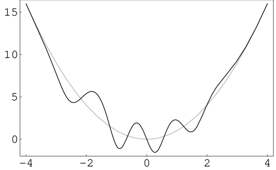
if is even but if is odd. It turns out
that is isospectral to the oscillator potential, a case
illustrated in figure 1 for () and . Let
us notice the already involved explicit expression of in
(46).
Figure 1: The confluent 2-SUSY partner potential (black
curve) isospectral to the oscillator (gray curve) generated by employing
the normalized eigenfunction (45) for and .
In turn, for the asymptotically vanishing
Schrödinger solutions become:
(47)
where is the Kummer hypergeometric series. The explicit
expression for is too involved to be shown here (three infinite
sums of kind (46) arise in this case). Alternatively, we performed
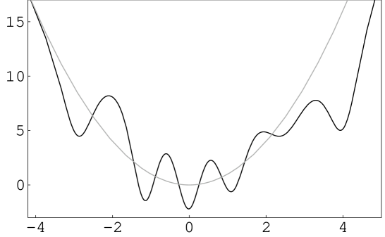
a numeric calculation of for taking the
solution of (47) with the upper plus sign and ,
in (19) (see figure 2). The spectrum of is
composed of the oscillator eigenenergies plus a
new level at . This illustrates clearly the possibility
offered by the confluent 2-SUSY algorithm of creating one single level
above the ground state energy of .
Figure 2: The confluent 2-SUSY partner potential
(black curve) of the oscillator (gray curve) generated by employing the
Schödinger solution (47) with the upper sign and
. The potential has an extra
bound state at compared with the oscillator spectrum.
We conclude that the second order supersymmetric quantum mechanics is a
powerful tool for designing in a simple way potentials with given spectra,
a subject supplying us of solvable models with possible applications in
the physical sciences (see e.g. [24]).
Acknowledgements.
The support of CONACYT (México) is acknowledged. One of the authors
(ESH) also acknowledges the financial support of the Instituto
Politécnico Nacional.
References
[1] AA Andrianov, MV Ioffe, VP Spiridonov, Phys. Lett. A 174 (1993) 273
[2] AA Andrianov, MV Ioffe, F Cannata, JP Dedonder, Int. J.
Mod. Phys. A 10 (1995) 2683
[3] BF Samsonov, Mod. Phys. Lett. A 11 (1996) 1563
[4] DJ Fernández, Int. J. Mod. Phys. A 12 (1997) 171
[5] DJ Fernández, ML Glasser, LM Nieto, Phys. Lett. A 240 (1998) 15
[6] JO Rosas-Ortiz, J. Phys. A 31 (1998) L507; ibid31 (1998) 10163
[7] JI Díaz, J Negro, LM Nieto, O Rosas-Ortiz, J. Phys.
A 32 (1999) 8447
[8] H Aoyama, N Nakayama, M Sato, T Tanaka, Phys. Lett. B
521 (2001) 400
[9] BF Samsonov, Phys. Lett. A 263 (1999) 274
[10] DJ Fernández, J Negro, LM Nieto, Phys. Lett. A 275
(2000) 338
[11] DJ Fernández, B Mielnik, O Rosas-Ortiz, B.F.
Samsonov, Phys. Lett. A 294 (2002) 168
[12] DJ Fernández, B Mielnik, O Rosas-Ortiz, BF Samsonov,
J. Phys. A 35 (2002) 4279
[13] DJ Fernández, R Muñoz, A Ramos, Phys. Lett. A 308 (2003) 11
[14] B Mielnik, LM Nieto, O Rosas-Ortiz, Phys. Lett. A. 269 (2000) 70
[15] IF Márquez, J Negro, LM Nieto, J. Phys. A 31
(1998) 4115
[16] PB Abraham, HE Moses, Phys. Rev A 22 (1980) 1333
[17] MM Nieto, Phys. Lett. B 145 (1984) 208
[18] CV Sukumar, J. Phys. A 18 (1985) 2937
[19] VB Matveev, MA Salle, Darboux transformations and
solitons, Springer-Verlag, Berlin (1991)
[20] BN Zakhariev, AA Suzko, Direct and inverse problems.
Potentials in quantum scattering, Springer-Verlag, Berlin (1990)
[21] J Pappademos, U Sukhatme, A Pagnamenta, Phys. Rev. A 48 (1993) 3525
[22] AA Stahlhofen, Phys. Rev. A 51 (1995) 934
[23] A Erdélyi, Higher transcendental functions v.1,
Mc-Graw Hill, New York (1953)
[24] E Drigo-Filho, JR Ruggiero, Phys. Rev. E 56 (1997)
4486