[

Scatterer that leaves ”footprints” but no ”fingerprints”

Abstract

We calculate the exact transmission coefficient of a quantum wire in the presence of a single point defect at the wire’s cut-off frequencies. We show that while the conductance pattern (i.e., the scattering) is strongly affected by the presence of the defect, the pattern is totally independent of the defect’s characteristics (i.e., the defect that caused the scattering cannot be identified from that pattern).

]

One of the most common ways to investigate the inner structure of a system is to perform scattering studies. That is, by looking at the scattering pattern one can cull some notion about the scatterer that was the cause of the specific scattering pattern. Our experience shows that every scatterer has a different scattering pattern. That explains the ubiquity of scattering techniques in the diagnostic world: for crystallographic studies, x-rays are used; visible light is usually used to detect molecule energy levels; ultrasound waves are commonly used for embryo imaging, etc.

In this paper, we discuss a case of a narrow wire in which our experience (that every scatterer has a different scattering pattern) fails. In this case, the scatterer has a strong influence on the dynamics of the system, both in terms of conductance (either high or low) and on the conduction pattern. However, the conductance and the scattering pattern are totally independent of the scatterer. The scatterer’s elusive conduct can be phrased: One can see the scatterer’s ”footprints” (its strong influence), but cannot see its ”fingerprints” (anything that may assist to characterize it).

When we think of a small and weak scatterer, the thing we usually have in mind is a scatterer whose influence on scattering is negligible. One of the reasons for this is that we are accustomed to a 3D world. In this case, the cross section is $\sigma\sim V^{2}$ (see ref.[1]), where $V$ is the scatterer strength (potential), i.e., it vanishes with scatterer potential. In 1D, however, this is definitely not the case. It is well known that when the incident particles’ energy is considerably lower (see below) than the scatterer’s strength (i.e., the scatterer’s potential), most of the incident particles are reflected from the scatterer, i.e., the scattering is strong regardless of scatterer ”weakness” (so long, of course, as the particles’ energy is lower than the scatterer’s potential). This behavior can be presented easily in the case of a weak scatterer, in which the reflection coefficient is related to the 1D scattering cross section. By using the term ”weak scatterer” we refer to the case in which its strength (its weak potential $\Delta V$) and its width ($L$) satisfy $\sqrt{\Delta V}L\ll 1$ (with the units $\hbar=2m=1$). In this case, the reflection coefficient maintains

$$R\simeq\frac{1}{1+4\omega/\left(\Delta VL\right)^{2}}$$ (1)

where $\omega$ is the energy of the incident particles. One can easily be convinced, though quite surprisingly, that the extreme case of the infinitely shallow potential barrier is actually the 1D delta function. That is, for the potential barrier $\alpha\delta\left(x\right)$ (or, the limit of $\Delta V=\alpha/L$ for $L\rightarrow 0$), the reflection coefficient reads

$$R=\frac{1}{1+4\omega/\alpha^{2}}$$ (2)

(notice, that now this is an equation and not merely an approximation). Eqs. (1) and (2) despite their simplicity, hold some peculiarities, which cannot be found in 3D scattering. These peculiarities can be summarized in three points:

1. The scattering is increased when the energy decreases.

2. The scattering is strong despite the scatterer’s ”weakness”.

3. The scattering for $\omega\rightarrow 0$ is independent of the scatterer (it does not depend on $\alpha$).

The third point is probably the most peculiar, since it contradicts our statement that each scatterer has a distinct scattering pattern. However, in 1D this feature is hardly interesting since it is valid only for zero incident particle energy ($\omega=0$). A particle with zero energy has little chance of even reaching the scatterer. In quasi-1D systems, the situation can be quite different.

In the case of the thin wire, for example, there are an infinite number of threshold (cut-off) energies. When the incident particles have exactly the cut-off energy of the $m$th mode, no energy is transferred to it (to the $m$th mode), since the momentum (or the k-vector) of this mode in the propagation direction is zero. Therefore, it makes sense to expect to find all the peculiarities of the 1D case, even in a 2D wire, near the threshold energies.

For such a system (point impurity in a quasi-1D wire) the 2D Scrödinger equation is

$$\nabla^{2}\psi+\left(\omega-V\right)\psi=-D\left(\mathbf{r}-\mathbf{r}_{0}\right)\psi$$ (3)

(where we use the units $\hbar=2m=1$). $V$ is the potential of the wire walls ($V=0$ inside the wire and $V=\infty$ outside it), $D$ is the defect potential and $\mathbf{r}_{0}=\varepsilon\hat{y}$ is the impurity location (see Fig.1). Since the defect has the proprties of a point-like impurity, the right-hand term of the Scrödinger equation can be written $D\left(\mathbf{r}-\mathbf{r}_{0}\right)\psi\left(\mathbf{r}_{0}\right)$ [2], which allows for an exact scattering solution.

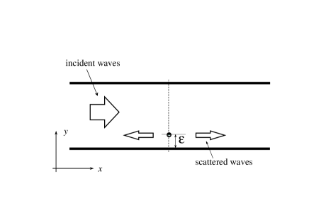
FIG. 1.: A 2D wire with a single point defect (black dot)

Let us assume that we hit the impurity with the incident wave $\psi_{inc}$. Taking advantage of the point-like nature of the impurity, the scattered wave function due to the defect is [3, 11]

$$\psi_{sc}=\psi_{inc}-\frac{\psi_{inc}\left(\mathbf{r}_{0}\right)\int d{\mathbf{r^{\prime}}}D\left({\mathbf{r^{\prime}}}-{\mathbf{r}}_{0}\right)}{1+\int d{\mathbf{r^{\prime}}}G^{+}\left({\mathbf{r^{\prime}}},{\mathbf{r}}_{0}\right)D\left(\mathbf{r}^{\prime}\mathbf{-r}_{0}\right)}G^{+}\left(\mathbf{r,r}_{0}\right)$$ (4)

where $G^{+}\left(\mathbf{r^{\prime},r^{\prime\prime}}\right)$ is the ”outgoing” 2D-Green function of the geometry (the wire). It should be noted that eq. 4 is an exact solution, however if the impurity were not an ideal point impurity, this equation would be a first-order approximation in the asymptotic solution $|\mathbf{r}\rightarrow\infty|$. The Green function for the given wire geometry takes the form:

$$\begin{array}[]{l}G\left(\mathbf{r,r^{\prime}}\right)=\\ i\sum_{n=1}^{\infty}\frac{\sin(n\pi y)\sin(n\pi y^{\prime})}{\sqrt{\omega-(n\pi)^{2}}}\exp\left[i\sqrt{\omega-(n\pi)^{2}}|x-x^{\prime}|\right]\end{array}$$ (5)

where ${\mathbf{r}}\equiv x\hat{x}+y\hat{y}$ and ${\mathbf{r^{\prime}}}\equiv x^{\prime}\hat{x}+y^{\prime}\hat{y}$. Hereinafter, the length parameters are normalized to the wire’s width.

Choosing the right potential for the impurity is a very tricky business as can be understood from the literature [4, 5, 6, 7, 8, 9, 10]. A simple 2D delta function (2DDF), which is a natural candidate to represent a point impurity (like in 1D), i.e., $\delta\left(x\right)\delta\left(y\right)$ does not scatter (its cross section is zero). Throughout this article we us the Impurity D Function (IDF) that was first presented by Azbel [2]. However, since in our wire’s geometry the problem’s symmetry is Cartesian rather than radial, we choose the following IDF:

$$D\left(\mathbf{r}\right)\equiv\lim_{\rho\rightarrow 0}\frac{2\sqrt{\pi}\delta\left(x\right)}{\rho\ln\left(\rho/\rho_{0}\right)}\exp\left(-y^{2}/\rho^{2}\right).$$ (6)

Unlike the 2DDF, this potential, which is infinitely shallower than the 2DDF, does scatter[2]. The de-Broglie wavelength of the impurity’s bound state is $\lambda_{B}=\pi\rho_{0}\exp(\gamma/2)/2$ (where $\gamma\simeq 0.577$ is the Euler constant). This is the only parameter that characterizes the impurity, and therefore eq. 6 can be used to mimic any impurity with the same de-Broglie wavelength, where its width is much smaller than $\lambda_{B}$.

On the face of it, the solution is straightforward: simply to substitute eqs. 6 and 5 into eq. 4. The problem is that the Green function has a logarithmic singularity at $|\mathbf{r-r^{\prime}}|\rightarrow 0$. Here is where the impurity’s width $\rho$ plays a major part, and the limit $\rho\rightarrow 0$ should be taken with great caution. Therefore, we first solve the integral for a finite $\rho$ and only then evaluate the limit.

Let us assume that the incident wave is the $n$th mode, and that the incident energy is close to the $m$th threshold energy (i.e., $\omega\simeq(m\pi)^{2}$ ) therefore,

$$\psi_{inc}\left(\mathbf{r}\right)=\sin(n\pi y)\exp\left(i\sqrt{\omega-(n\pi)^{2}}x\right).$$ (7)

The probability density of Eq.(7) is presented in Fig.2 for $n=1$ and $m=2$.

By using the following relation

$$\begin{array}[]{r}\int_{-\infty}^{\infty}dy\sin(n\pi y)\exp\left[-(y-\varepsilon)^{2}/\rho^{2}\right]=\\ \rho\sqrt{\pi}\sin(n\pi\varepsilon)\exp\left[-(n\pi\rho/2)^{2}\right]\\ \end{array}$$ (8)

We find the solution (for $x>0$)

$$\psi_{sc}\left(\mathbf{r}\right)=\sum_{l=1}^{\infty}\left(\delta_{nl}-A_{nl}\right)\sin(l\pi y)\exp\left(i\sqrt{\omega-(l\pi)^{2}}x\right)$$ (9)

where $\delta_{nl}$ is the Kronecker delta and

$$A_{nl}\equiv\frac{\sin(n\pi\varepsilon)\sin(l\pi\varepsilon)}{i\sqrt{\omega-(l\pi)^{2}}\left[\frac{\ln(\rho_{0}/\bar{\rho})}{2\pi}+\sum_{n^{\prime}\leq m}\frac{\sin^{2}(n^{\prime}\pi\varepsilon)}{i\sqrt{\omega-(n^{\prime}\pi)^{2}}}\right]}$$ (10)

and $\bar{\rho}$ is some length scale which depends on the impurity’s location ($\varepsilon$), the incident energy $\omega$ and $m$:

$$\ln(\bar{\rho})\equiv\lim_{\rho\rightarrow 0}\left\{\ln\rho+2\pi\sum_{n^{\prime}=m+1}^{\infty}\frac{\sin^{2}(n^{\prime}\pi\varepsilon)}{\sqrt{(n^{\prime}\pi)^{2}-\omega}}e^{-(n^{\prime}\pi\rho/2)^{2}}\right\}$$ (11)

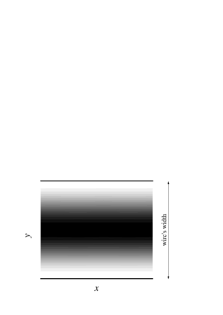
FIG. 2.: The probability density distribution in the wire for $n=1$ and $\omega=(2\pi)^{2}$ in the absence of the point defect.

In this paper we discuss the case where $\omega\simeq(m\pi)^{2}$ for any integer $m$ (though the figures are focused on the case $\omega\simeq(2\pi)^{2}$, i.e., $m=2$). In this particular case only the $n$th mode (the incident mode) and the $m$th one have a considerable influence on the scattering

$$\psi_{sc}\simeq\psi_{inc}-\frac{\sin(n\pi\varepsilon)}{\sin(m\pi\varepsilon)}\frac{\sin(m\pi y)e^{i\sqrt{\omega-(m\pi)^{2}}|x|}}{1+i\sqrt{\omega-(m\pi)^{2}/\Delta_{m}}}$$ (12)

where

$$\Delta_{m}^{-1/2}\equiv\frac{\ln(\rho_{0}/\bar{\rho})}{2\pi\sin^{2}(m\pi\varepsilon)}-i\sum_{n^{\prime}<m}\frac{\sin^{2}(n^{\prime}\pi\varepsilon)}{\sin^{2}(m\pi\varepsilon)}\frac{1}{\pi\sqrt{m^{2}-n^{\prime 2}}}$$ (13)

The scattered wave function, i.e., Eq.(12), depends on the scatterer’s parameter ($\rho_{0}$) only via $\Delta_{m}$. Therefore, when

$$(\omega-(m\pi)^{2})/\Delta_{m}\ll 1$$ (14)

one finds:

1) When the energy is not close to the threshold energy, the scattering is negligible; as we get closer to the threshold energy, the scattering increases.

2) The scattering coefficient is large (can have any value) regardless of the scatterer’s ”weakness”.

3) Near the threshold energies, the scattering is independent of the scatterer (it does not depend on the scatterer’s parameter).

Again, the most bizarre behavior is the third one, which is manifested in the limit $\omega\rightarrow(m\pi)^{2}$ of Eq.(12) (see Fig.3):

$$\psi_{sc}=\psi_{inc}-\frac{\sin(n\pi\varepsilon)}{\sin(m\pi\varepsilon)}\sin(m\pi y)$$ (15)

Eq.(15), which present the scattering of the $n$th mode, when its energy is equal to the threshold energy of the $m$th one, can be generalized for a wire with an arbitrary (but uniform) cross section

$$\psi_{sc}=\chi_{n}(y)e^{i\sqrt{\omega_{m}-\omega_{n}}x}-\frac{\chi_{n}(\varepsilon)}{\chi_{m}(\varepsilon)}\chi_{m}(y)$$ (16)

where $\chi_{n}(y)$ is the transversal eigenstates of the wire, with the corresponding eigen energies $\omega_{n}$.

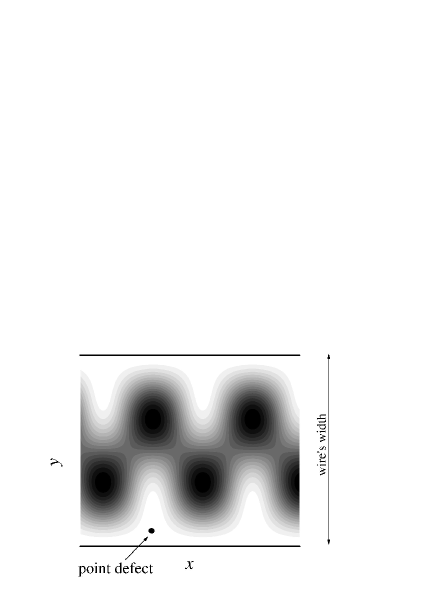
FIG. 3.: The probability density distribution in the wire for $n=1$ and $\omega=(2\pi)^{2}$ when the point defect is present.

While Eq.(12) is an approximation, Eqs.(15) and (16) are totally accurate for any point impurity, and at any impurity’s location.

In the case of a surface impurity, i.e., $\varepsilon\rightarrow 0$ (or $\varepsilon\rightarrow 1$), eq. (12) is reduced to an even simpler one

$$\psi_{sc}\simeq\psi_{inc}\mp\left(\frac{n}{m}\right)\frac{\sin(m\pi y)e^{i\sqrt{\omega-(m\pi)^{2}}|x|}}{1+i\sqrt{\omega-(m\pi)^{2}/\Delta_{m}}}$$ (17)

where

$$\Delta_{m}^{-1/2}\simeq\frac{\ln(\rho_{0}/C\varepsilon)}{2\pi(m\pi\varepsilon)^{2}}$$ (18)

and

$$C\equiv 4\exp\left[\gamma/2-\mathrm{Ci}(\pi)\right]\simeq 5$$ (19)

is a numerical constant (Ci is the cosine integral). The upper sign (minus) in eq.(17) stands for impurity at the lower boundary $\varepsilon\ll m^{-1}$ while the plus implies an upper boundary impurity $1-\varepsilon\ll m^{-1}$ (in this case the $\varepsilon$ should be replaced by $1-\varepsilon$ in eq.18).

Thus, at the threshold energy, i.e., $\omega=(m\pi)^{2}$,

$$\psi_{sc}=\sin(m\pi y)e^{i\pi\sqrt{m^{2}-n^{2}}x}\mp\left(\frac{n}{m}\right)\sin(m\pi y)$$ (20)

That is, in the case of a surface impurity then close enough to the threshold energies (i.e., when eq.(20) holds) the scattering is also independent of the impurity’s location. Any impurity’s characteristics have faded away near the threshold energies. Eq.(20) does not reflect any feature of the scatterer: it depends neither on its strength nor on its location.

It was shown in the literature (see, for example, ref.[4]) that at the threshold energies, the conductance is totally quantized and is independent of the point defects, however, here we show two additional results:

the scattering is not a negligible quantity, it does not affect the conductance but it does distort the conduction pattern; and at the same time, that this severe distortion is independent of the scatterer that caused it.

It should be stressed that while the discussion was focused on quantum wire, this effect can occur in any waveguide with a single point scatterer: acoustical waveguide, electromagnetic waveguide, optical waveguide, etc.

I am grateful to Mark Azbel for enlightening discussions.

REFERENCES

- [1] E. Merzbacher, ”Quantum Mechanics”, (Wiley 1970)
- [2] M.Ya. Azbel, Phys. Rev. B 43, 2435 (1991); 43, 6717 (1991); Phys. Rev. Lett 67, 1787 (1991)
- [3] E. Granot and M.Ya. Azbel, Phys. Rev. B 50, 8868 (1994)
- [4] C.S. Chu and R.S. Sorbello, Phys. Rev. B 40, 5941 (1989)
- [5] A. Kumar and F. Bagwell, Phys. Rev. B 43, 9012 (1991)
- [6] P.F. Bagwell, Phys. Rev. B 41, 10354 (1990)
- [7] Y.B. Levinson, M.I. Lubin, and E.V. Sukhorukov, Phys. Rev. B 45, 11936 (1992)
- [8] S.A. Gurvitz and Y.B. Levinson, Phys. Rev. B 47, 10578 (1993)
- [9] E. Tekman and S. Ciraci, Phys. Rev. B 42,9098 (1990)
- [10] C.S. Kim and A.M. Satanin, Physica E 4, 211 (1999)
- [11] E. Granot, Phys. Rev. B 60, 10664 (1999); 61, 11078 (2000)