Three routes to the exact asymptotics for the one-dimensional quantum walk

Abstract

We demonstrate an alternative method for calculating the asymptotic behaviour of the discrete one-coin quantum walk on the infinite line, via the Jacobi polynomials that arise in the path integral representation. We calculate the asymtotics using a method that is significantly easier to use than the Darboux method. It also provides a single integral representation for the wavefunction that works over the full range of positions, $n,$ including throughout the transitional range where the behaviour changes from oscillatory to exponential. Previous analyses of this system have run into difficulties in the transitional range, because the approximations on which they were based break down here. The fact that there are two different kinds of approach to this problem (Path Integral vs. Schrödinger wave mechanics) is ultimately a manifestation of the equivalence between the path-integral formulation of quantum mechanics and the original formulation developed in the 1920s. We also discuss how and why our approach is related to the two methods that have already been used to analyse these systems.

1 Introduction

The discrete quantum walk has been discussed in several recent papers [12, 3]. The first authors to discuss the quantum random walk were Y. Aharonov, Davidovich and Zagury, in [2] where they described a very simple realization of the quantum random walk in quantum optics. Some further early results were due to Meyer, in [11]. He proved that for a discrete (unitary) quantum walk on the line to have non-trivial behaviour, its motion must be assisted by an additional “coin” degree of freedom which is conventionally taken to be two dimensional. This spin-like degree of freedom is sometimes called the chirality, and can take the values RIGHT and LEFT, or a superposition of these. Meyer therefore considered the wave function as a two component vector of amplitudes of the particle being at point $n$ at time $t$. Let

$$\Psi(n,t)=\begin{pmatrix}\psi_{L}(n,t)\\ \psi_{R}(n,t)\end{pmatrix}$$ (1)

where we shall label the chirality of the top component LEFT and the bottom RIGHT. This paper is concerned with the dynamics of a test particle performing an unbiased quantum walk on the integer points on the line. At each time step the chirality of the particle evolves according to a unitary Hadamard transformation

$$|\rm{R}\rangle\mapsto\frac{1}{\sqrt{2}}(|\rm{R}\rangle+|\rm{L}\rangle)$$ (2)

$$|\rm{L}\rangle\mapsto\frac{1}{\sqrt{2}}(|\rm{R}\rangle-|\rm{L}\rangle)$$ (3)

and then the particle moves according to its (new) chirality state. Therefore, the particle obeys the recursion relations

$$\Psi_{\rm{L}}(n,t+1) =-\frac{1}{\sqrt{2}}\Psi_{\rm{L}}(n+1,t)+\frac{1}{\sqrt{2}}\Psi_{\rm{R}}(n-1,t)$$ (4)

$$\Psi_{\rm{R}}(n,t+1) =\frac{1}{\sqrt{2}}\Psi_{\rm{L}}(n+1,t)+\frac{1}{\sqrt{2}}\Psi_{\rm{R}}(n-1,t).$$ (5)

Meyer and subsequent authors have considered two approaches to the Hadamard walk, the Path Integral and Schrödinger approaches, which reflect two complementary ways of formulating quantum mechanics [8]. We refer to the paper by Ambainis, Bach, Nayak, Vishwanath and Watrous [3] for proper definitions and references. We shall refine the asymptotic analysis of this paper.

The behaviour of the Hadamard walk is very different from the classical random walk on the integer points on the real line. One way of understanding this is as a result of quantum interference. Destructive interference suppresses the probability amplitude in the vicinity of the origin, and constructive interference reinforces it away from the origin. The net effect of this is that the quantum walk spreads out much faster. Figure 1 shows the discrete quantum walk on the infinite line at $t=100.$ We have only plotted the distribution for even values of $n$ in Figure 1. If a walk’s initial distribution has its support confined to a set of nodes which all have the same parity (all $n$s either even or odd) the support of the distribution will “tick” between different parities at each step.

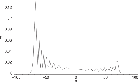
Figure 1: The discrete quantum walk on the line. The probability distribution is shown for a walk that started at the origin with its coin in the state $|\rm{R}\rangle$ after it has evolved for 100 steps. The distribution is oscillatory between the two peaks and decays exponentially outside that range. The peaks move away from the origin with speed $t/\sqrt{2},$ and the width of the peaks also decreases with time. By contrast, the classical random walk has a Gaussian distribution, which spreads with velocity $\sim\sqrt{t}.$

The probability distribution for the quantum walk depends not only on the evolution law in (2), but also on the initial conditions. Throughout this paper we will only consider walks that start at $n=0$ with the coin in the initial state $|\rm{R}\rangle.$ The convention that the walk starts in the position $n=0$ is inherited from the motivation for studying these systems as toy models of quantum algorithms: the computer is always started with its registers in the state $|00\ldots\rangle.$ The choice of initial coin state was made because the Hadamard walk is an unbiased walk [12]. This means that even though some starting conditions result in an asymmetric probability distribution, we can always find some other starting state that will produce a walk with the opposite bias. The $|\rm{R}\rangle$ starting state produces a distribution that is maximally biased to the right. Likewise, if we had chosen to start the walk in the state $|\rm{L}\rangle,$ this would have produced a distribution that was maximally biased to the left. This distribution is the exact mirror-image of that produced by starting in the state $|\rm{R}\rangle.$ Thus, reversing the starting condition just relabels $n$ to $-n.$ As the coin space is two-dimensional, we can now invoke the linearity of quantum mechanics, and note that we can obtain the behaviour for any initial condition $|\Phi\rangle=a|\rm{R}\rangle+b|\rm{L}\rangle$ by forming the corresponding linear combination of the evolutions for the initial condition basis states $|\rm{R}\rangle,|\rm{L}\rangle.$

2 Related Work

We now very briefly describe the methods previous authors have used. They have so far followed two approaches to determine the limiting behaviour of the $\psi$-functions as $t\rightarrow\infty$. The translational invariance of this problem means that it has a simple description in momentum space, and the Schrödinger approach relies on that fact. We will describe this in more detail in the section below. Beginning with the recursion relation (4), Nayak and Vishwanath [12] showed that

$$\tilde{\Psi}(k,t)=\left(M_{k}\right)^{t}\tilde{\Psi}(k,0)$$ (6)

where

$$\tilde{\Psi}(k,0)=\sum_{n}\Psi(n,0)e^{ikn}$$ (7)

and $M_{k}$ is the matrix

$$M_{k}=\frac{1}{\sqrt{2}}\begin{pmatrix}-e^{-ik}&e^{-ik}\\ e^{ik}&e^{ik}\end{pmatrix}.$$ (8)

They diagonalize the matrix $M_{k}$, finding the eigenvalues $\lambda_{k}^{1}=e^{i\omega_{k}}$ and $\lambda_{k}^{2}=e^{i(\pi-\omega_{k})}$ where $\omega_{k}=\arcsin\left(\frac{\sin k}{\sqrt{2}}\right),\quad\omega_{k}\in[-\pi/2,\pi/2]$. They then write the $\psi$-functions in terms of the eigenvalues $\left(\lambda_{k}^{1}\right)^{t}$ and $\left(\lambda_{k}^{2}\right)^{t}$ and their associated eigenvectors and formally invert the original fourier transform to obtain the closed form integral representations for the wavefunction,

$$\psi_{\rm{L}}(n,t) =\frac{1+(-1)^{n+t}}{2}\int_{-\pi}^{\pi}\frac{dk}{2\pi}(1+\frac{\cos k}{\sqrt{1+\cos^{2}k}})e^{-i(\omega_{k}t+kn)}$$ (9)

$$\psi_{\rm{R}}(n,t) =\frac{1+(-1)^{n+t}}{2}\int_{-\pi}^{\pi}\frac{dk}{2\pi}\frac{e^{ik}}{\sqrt{1+\cos^{2}k}}e^{-i(\omega_{k}t+kn)}.$$ (10)

They then approximate these, using a combination of the method of stationary phase in one range, and integration by parts in the other. (Note that the Left-Right labelling convention in [12] is the opposite to ours.)

There is another approach based on the Path Integral formulation of quantum mechanics, that Ambainis et al. discuss. The $\psi$-functions are expressed in terms of Jacobi polynomials (as in Lemma 2 below) of the form

$$J_{j}^{(aj+\gamma,bj+\beta)}(0),\;j=(t-n)/2-1=(1-\gamma)t/2-1.$$ (11)

One may then derive the asymptotic behaviour of the $\psi$-functions as $t\rightarrow\infty$ by determining the asymptotic behaviour of these Jacobi polynomials as $m\rightarrow\infty$. This has been done in two ways. Ambainis et al. use the approach due to Chen and Ismail [7], which employs the Darboux method. Here one begins with the Srivastava-Singhal generating function

$$\sum_{j=0}^{\infty}J_{j}^{(\gamma+aj,\beta+bj)}(w)z^{j}=(1+{\bf{u}})^{-\gamma}(1+{\bf{v}})^{-\beta}[1+(1+a){\bf{u}}+(1+b){\bf{v}}]^{-1}$$ (12)

where ${\bf{u}}$ and ${\bf{v}}$ are defined to be power series in $w$ that satisfy the equations

$${\bf{u}} =-\frac{1}{2}(w+1)z(1+{\bf{u}})^{-\lambda}(1+{\bf{v}})^{-\mu-1}$$ (13)

$${\bf{v}} =-\frac{1}{2}(w-1)z(1+{\bf{u}})^{-\lambda-1}(1+{\bf{v}})^{-\mu}.$$ (14)

Chen and Ismail use the Darboux method to calculate the asymptotics of these Jacobi polynomials. This method starts from the idea that if $f(z)=\sum_{n\geq 0}a_{n}z^{n}$ then the radius of convergence is $\mathcal{R}=\lim_{n\rightarrow\infty}\left(\frac{1}{|a_{n}|}\right)^{1/n}$ when this limit exists. Suppose there is a comparison function $g(z)=\sum_{n\geq 0}b_{n}z^{n}$ such that $g(z)-f(z)$ has a larger radius of convergence than $f(z),$ then $b_{n}-a_{n}=O(s^{-n})$ where $s>\mathcal{R}.$ If the asymptotic behaviour of $b_{n}$ is known, then since $a_{n}\sim b_{n}$ then we know the asymptotic behaviour of $a_{n}.$ Chen and Ismail use the Srivastava-Singhal description of the generating function for Jacobi polynomials to determine its singularities on the radius of convergence and give comparison functions at each singularity to determine the asymptotic behaviour of the Jacobi polynomials.

It is interesting to note that the reciprocals of these two singularities (when normalized by dividing by $\left(\sqrt{2}\right)^{t}$) are the eigenvalues that arise in the Schrödinger method.

3 Overview and Results

The other way to obtain the asymptotic behaviour of these Jacobi polynomials is to follow the method in Gawronkski and Shawyer’s paper, [9]. This is the third way to analyse these systems, and will be the way that we follow in much of this paper. It is a refinement of the methods in the paper by Saff and Varga [14]. This uses the method of steepest-descents. We will outline this method below but for further details we recommend [5, 16] and also the book by Olver [13] which describes both the steepest-descent method and the method of Darboux very clearly.

The saddle-points that feature in this method are also related to the eigenvalues that arise in the Schrödinger method. We will detail this relationship below. If $\zeta$ is a saddlepoint then $\exp(h(\zeta))$ is an eigenvalue from the Schrödinger method, for a function $h(\zeta)$ that we define below.

We now describe our results. We shall see that it is possible to obtain explicit asymptotic expansions that are uniformly convergent. The system displays two types of behaviour, with the transitions between the different behaviours governed by a parameter, $\alpha=n/t$. The behaviour changes qualitatively over three ranges, which are respectively $0\leq|\alpha|\leq\frac{1}{\sqrt{2}}-\varepsilon,\frac{1}{\sqrt{2}}-\varepsilon<|\alpha|<\frac{1}{\sqrt{2}}+\varepsilon,$ and $\frac{1}{\sqrt{2}}+\varepsilon\leq|\alpha|<1-\varepsilon$, where $\varepsilon$ is a positive number. Our methods give error terms of the form $O(t^{-N-1/2})$ where $N$ is some positive integer, and the expansion for each range holds uniformly. We stop at $O(t^{-5/2})$ since we have no application for the more precise estimates.

The first range is arguably the most interesting. Here the asymptotic behaviour of the $\psi$-functions is oscillatory as $t\rightarrow\infty$. We will use a result by Gawronkski and Shawyer [9] who obtained the leading term and the factor $1+O(t^{-1})$ for the error term for Jacobi polynomials. When this result is applied to the $\psi$-functions, we obtain a refinement of Theorem 2 of [3] who found the leading term.

The second, boundary, range is treated using the method of coalescing saddle-points as described in R. Wong’s book [16]. A uniform asymptotic expansion is possible which involves the Airy function. This is also interesting because the $\psi$-functions change from an oscillating, polynomially bounded asymptotic behaviour to an exponentially small behaviour as $|\alpha|$ changes from below $1/\sqrt{2}$ to above $1/\sqrt{2}$. The calculation of the asymptotics for these polynomials is novel to the best of the authors’ knowledge. The third range is the immediate vicinity of $|\alpha|=1/\sqrt{2}.$ As the behaviour of our integral representation is well understood, we can obtain uniformly convergent asymptotics thoughout this transitional range.

The main interest of our results lies not in the more accurate asymptotic expansions for the $\psi$-functions in the first and third ranges of $\alpha,$ although Ambainis et al. did ask for a uniform method to do the asymptotics for these ranges. In fact, Gawronkski and Shawyer have already provided this method [9]. The fact that the uniform asymptotic behaviour for the Jacobi polynomials for the transistion from polynomially bounded oscillating behaviour to exponential decay can be found in terms of the Airy function seems rather more interesting. It is somewhat surprising that this has not (to our knowledge) been published before for this family of polynomials: Wong’s book [16] shows how to obtain the asymptotic behaviour in terms of Airy functions. Perhaps the reason for this omission is simply the previous lack of an application, which the quantum walk now provides.

4 The Feynman Path Integral

We begin with the Feynman path integral appproach following Meyer. We will represent the components of the vector-valued wavefunction as a normalized sum over signed paths. Meyer [11] proved

Lemma 1 (Meyer [11]).

Let $-n\leq t<n$. Define $l=\frac{t-n}{2}$. The amplitudes of position $n$ after $t$ steps of the Hadamard walk are:

$$\psi_{R}(n,t) =\frac{1}{\sqrt{2^{t}}}\sum_{s}\binom{l-1}{s-1}\binom{t-l}{s}(-1)^{t-s}$$ (15)

$$\psi_{L}(n,t) =\frac{1}{\sqrt{2^{t}}}\sum_{s}\binom{l-1}{s}\binom{t-l}{s}(-1)^{t-s-1},$$ (16)

except for the endpoints where $t=n,$ which have to be handled separately.

(See [11] for the endpoints. For a derivation of these formulae, see Appendix A of [6].)

We will follow the approach used by Ambainis et al. [3] and Meyer [11] but in greater detail to obtain the following lemma. The standard notation in [1] for Jacobi polynomials is to write them as $J_{n}^{(\alpha,\beta)}(z),$ but to avoid confusion with $\alpha=n/t$ we will write these as $J_{r}^{(u,v)}(z).$ (Note that in the following lemma, we have reintroduced the external phase that was omitted in [11] and [3].)

Lemma 2 (Ambainis et al.[3]).

When $n\equiv t$ mod 2 and $J_{r}^{(u,v)}(z)$ denotes a Jacobi polynomial,

$$\psi_{R}(n,t)(-1)^{(t-n)/2}=\begin{cases}-(\frac{t+n}{t-n})2^{-n/2-1}J_{(t-n)/2-1}^{(1,n)}(0),&\text{ when }0\leq n<t\\ -2^{n/2-1}J_{(t+n)/2-1}^{(1,-n)}(0),&\text{ when }-t\leq n<0.\end{cases}$$ (17)

Also,

$$\psi_{L}(n,t)(-1)^{(t-n)/2}=\begin{cases}(-1)^{n+1}2^{-n/2-1}J_{(t-n)/2-1}^{(0,n+1)}(0),&\text{ when }0\leq n<t\\ (-1)^{n+1}2^{n/2}J_{(t+n)/2}^{(0,-n-1)}(0),&\text{ when }-t\leq n<0.\end{cases}$$ (18)

Remark: As Ambainis et al. [3] point out

$$\psi_{L}(-n,t)=-\psi_{L}(n-2,t), \psi_{R}(-n,t)=\frac{t-n}{t+n}\psi_{R}(n,t).$$ (19)

Proof of Lemma 2: We use two formulae from Abromowitz and Stegun [1] to prove these results. The first is the Pfaff-Kummer transformation [4] (15.3.4 of [1])

$$\;_{2}F_{1}(a,b;c;z)=(1-z)^{-a}\;_{2}F_{1}(a,c-b;c;\frac{z}{z-1}).$$ (20)

The second is the representation of a Jacobi polynomial as a $\;{}_{2}F_{1}$, see 15.4.6 of [1]

$$\;_{2}F_{1}(-j,u+1+v+j;u+1;z)=\frac{j!}{(u+1)_{j}}J_{j}^{(u,v)}(1-2z).$$ (21)

Now the first sum, say $S,$ in Lemma 1 is $\;{}_{2}F_{1}(1-l,-(t-l);1;-1)$ so by (20)

$$S=2^{(t-n)/2-1}\;_{2}F_{1}(1-(t-n)/2,-1+(t-n)/2+n+1+1;1;1/2).$$ (22)

Now by (21) we obtain

$$S=2^{(t-n)/2-1}J_{(t-n)/2-1}^{(0,n+1)}(0).$$ (23)

This proves the first part of Lemma 2 for $n\geq 0.$ To derive the second part, for $n<0$ we see

$$S=\;_{2}F_{1}(-(t+n)/2,1-1+(n-t)/2;1;-1)\\ =2^{(t+n)/2}\;_{2}F_{1}(-(t+n)/2,1+(n+t)/2-n-1;1;1/2)=2^{(t+n)/2}J_{(t+n)/2}^{(0,-n-1)}(0).$$ (24)

The results for the first sum are now proved.

The second sum, say $T$, can be treated in much the same way since

$$T=(l-t)\;_{2}F_{1}(1-l,l-t+1;2;-1)=2^{l-1}(l-t)\;_{2}F_{1}(1-l,2-l+t-1;2;1/2)\\ =2^{(t-n)/2-1}(l-t)\;_{2}F_{1}(-(l-1),2+l-1+n;2;1/2)\\ =(l-t)2^{(t-n)/2-1}J_{(t-n)/2-1}^{(1,n)}(0)/l.$$ (25)

The result for nonnegative $n$ now follows. If $n$ is negative

$$T=\;_{2}F_{1}(-(n+t)/2+1,1-l;2;-1)\frac{t+n}{2}\\ =\frac{t+n}{2}2^{(t+n)/2-1}\;_{2}F_{1}(-(t+n)/2-1,2+(n+t)/2-1-;2;1/2)\\ =\frac{t+n}{2}2^{(t+n)/2-1}\;_{2}F_{1}(-((t+n)/2-1),2+((n+t)/2-1)-t;2;1/2)\\ =\frac{t+n}{t+n}2^{(t+n)/2-1}J_{(t+n)/2-1}^{(1,-n)}(0).$$ (26)

This completes the proof of Lemma 2.

We consider first of all $\psi_{L}(n,t),\;n\geq 0.$ (As was observed by Ambainis et al., there is a symmetry between positive and negative $n$.) We let

$$m=(1-\alpha)t/2-1$$ (27)

so that

$$1+n=1+\alpha t=\frac{1+\alpha}{1-\alpha}+\frac{2\alpha}{1-\alpha}m$$ (28)

and

$$J_{(1-\alpha)t/2-1}^{(0,n+1)}(0)=J_{m}^{(0+0\cdot m,\frac{1+\alpha}{1-\alpha}+\frac{2\alpha m}{1-\alpha})}(0).$$ (29)

4.1 The oscillatory range:$|\alpha|<1/\sqrt{2}-\varepsilon$

For $0\leq\alpha<2^{-1/2}-\varepsilon,\quad 0<\varepsilon\leq 2^{-1/2},$ we may use either the Chen-Ismail [7] results or the Gawronkski-Shawyer [9] results. We use the results by Gawronkski and Shawyer since they have been proved to hold uniformly over this range of $\alpha.$ For the sake of consistency of notation and ease of reference we will state the Gawronkski and Shawyer result in a more restricted form than they obtained in their paper, but it is sufficient for our purposes.

Gawronkski and Shawyer write, using the integral representation in equation (4.46) of Szegö’s book [15],

$$J_{m}^{(am+\gamma,bm+\beta)}(z)=\frac{1}{2\pi i}\int_{\Gamma}e^{mh(\zeta)}g(\zeta)d\zeta$$ (30)

where

$$h(\zeta) =\ln\left(\frac{\zeta^{2}-1}{2(\zeta-z)}\right)+a\ln\left(\frac{1-\zeta}{1-z}\right)+b\ln\left(\frac{1+\zeta}{1+z}\right)$$ (31)

$$g(\zeta) =\left(\frac{1-\zeta}{1-z}\right)^{\gamma}\left(\frac{1+\zeta}{1+z}\right)^{\beta}\frac{1}{\zeta-z}$$ (32)

and $\Gamma$ is a contour circling the origin. These integrals are of the form

$$I(m)=\int_{\Gamma}g(\zeta)e^{-mh(\zeta)}\;d\zeta$$ (33)

and as such can be approximated in the limit as $m\to\infty$ using the method of steepest descents [5, 13, 16]. This relies the fact that in this limit (i.e., $t\to\infty$) the only parts of the integrand that contribute significantly to the integral are those regions where the function in the exponent, $h,$ has a maximum. This is because in the long time limit the exponential term in the integrand behaves more and more like $\delta$-function(s) centred on point(s) where $h$ is maximal. (Note that a stationary point of $h$ is only a maximum along a given contour of integration, $\Gamma.$ This is because the stationary points of an analytic function can only be saddle-points, so whether they appear to be maxima or minima depends on the path taken through them.)

In order to make use of this phenomenon, we need to be able to assume that the imaginary part of $h$ is approximately constant in the vicinity of these saddle-points, otherwise the integrand will oscillate unmanageably in the asymptotic limit. (We don’t care if it oscillates wildly elsewhere, as the contribution from those regions will be negligibly small.) The way to achieve this is to choose the contour so that it passes through these saddle-points along the path of steepest descent for the real part of the exponent.

We therefore choose the path $\Gamma$ so it goes through the two saddle-points $\zeta^{+},\zeta^{-}$ determined by

$$h^{\prime}(\zeta)=0(\text{ or }(1+\alpha)\zeta^{2}-2\alpha\zeta+1-\alpha=0).$$ (34)

Thus the imaginary part of $h(\zeta)$ is fixed which implies that the real part of $h(\zeta)$ has a maximum at the saddle-point. (The numbers $e^{h(\zeta^{+})},e^{h(\zeta^{-})}$ are the reciprocals of the singularities found by Chen and Ismail using Darboux’s method.) Gawronkski and Shawyer use a steepest descent contour which goes through the saddle-points at $\zeta=\zeta^{+}$ or $\zeta^{-}$ and the points $\zeta=\pm 1.$ The contour must be modified slightly near the singularities at $\zeta=\pm 1.$ The contours are leaf-shapes defined by

$$\Im(h(\zeta))=\Im(h(\zeta^{+})).$$ (35)

So (for example) when $\alpha=1/2$ this is

$$\Im(\ln(\zeta^{2}-1)-\ln 2-\ln\zeta+2\ln(1+\zeta))=\Im(\ln((\zeta^{+})^{2}-1)-\ln 2-\ln\zeta^{+}+2\ln(1+\zeta^{+}))$$ (36)

where

$$\zeta^{+}=\frac{\alpha+i\sqrt{1-2\alpha^{2}}}{1+\alpha}=\frac{1+i\sqrt{2}}{3}.$$ (37)

Figure 2 is an example of the steepest descent curve for the oscillatory range of $\alpha.$

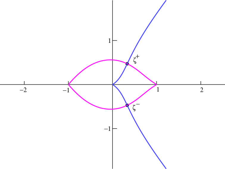
Figure 2: Steepest descent and ascent curves for the oscillatory range of $\alpha.$ The descent curve is the leaf-shape, and the two lines running off to $\pm\infty$ are the steepest ascent curves.

The Gawronkski and Shawyer result is stated in terms of the parameters $A,B,D,C_{1},C_{2},\theta,\rho(\theta)$ and $\xi(\theta)$ defined as follows:

$$\cos\theta=-\frac{\alpha^{2}}{1-\alpha^{2}}\quad\quad\text{ so }\quad\frac{\pi}{2}\leq\theta<\pi,$$ (38)

$$A=0,\quad\quad B=\alpha,\quad\quad D=1-\alpha^{2},$$ (39)

$$C_{1}=1,\quad C_{2}=\frac{1+\alpha}{1-\alpha}.$$ (40)

They then show that $\rho(\theta)$ increases monotonically from $0$ to $\pi$ as $\theta$ increases from $0$ to $\pi$ or equivalently as $|\alpha|$ increases from $0$ to $1/\sqrt{2}$. Furthermore

$$\rho(\theta) =\theta+\frac{2\alpha}{1-\alpha}\left(\frac{\theta}{2}-\arctan\left(\frac{1+B^{2}-D}{2B}\tan\theta/2\right)\right),$$ (41)

$$\xi(\theta) =\frac{\theta}{2}+\frac{\pi}{4}+\frac{1+\alpha}{1-\alpha}\left(\frac{\theta}{2}-\arctan\left(\frac{1+B^{2}-D}{2B}\tan\theta/2\right)\right).$$ (42)

Here $-\pi/2<\arctan u<\pi/2$ for real $u$.

Theorem 1 (Gawronkski and Shawyer [9]).

$$J_{m}^{(0+0\cdot m,\frac{1+\alpha}{1-\alpha}+\frac{2\alpha m}{1-\alpha})}(0)=\left(\pi m(1+B)\sin\theta/2\cos\theta/2\right)^{-1/2}\times\\ \left(C_{2}^{-1}(1+B)\left((C_{2}-1)^{2}/4+C_{2}\cos^{2}\theta/2\right)^{1/2}\right)^{-\frac{2\alpha m}{1-\alpha}-\frac{1+\alpha}{1-\alpha}}\left(\sin(m\rho(\theta)+\xi(\theta))+O(1/m)\right)$$ (43)

as $m$ (i.e., $t$) $\rightarrow\infty$.

Now, by direct substitution,

$$\left(\pi m(1+B)\sin(\theta/2)\cos(\theta/2\right)^{-1/2} =2\left(\frac{1}{\pi t\sqrt{1-2\alpha^{2}}}\right)^{1/2}$$ (44)

$$C_{2}^{-1}(1+B) =1-\alpha$$ (45)

$$\left((C_{2}-1)^{2}/4+C_{2}\cos^{2}(\theta/2)\right)^{1/2} =\frac{1}{\sqrt{2}(1-\alpha)}$$ (46)

Thus from equations (43),(44),(45) and (46),

$$J_{m}^{(0,2\alpha/(1-\alpha)+(1+\alpha)/(1-\alpha))}(0)=2\left(\frac{1}{\pi t\sqrt{1-2\alpha{{}^{2}}}}\right)^{1/2}\times\\ 2^{(2\alpha((1-\alpha)t-1))/(1-\alpha)+(1+\alpha)/(1-\alpha))/2}\sin\left((1-\alpha)t/2-1)\rho(\theta)+\xi(\theta)\right)(1+O(1/t)).$$ (47)

We have that

$$\alpha t-\frac{\alpha}{1-\alpha}+\frac{1+\alpha}{2(1-\alpha)}=\frac{\alpha t}{2}+\frac{1}{2}$$ (48)

so

$$J_{m}^{(0,\frac{2\alpha m}{1-\alpha}+\frac{1+\alpha}{1-\alpha})}(0)=\frac{2\sqrt{2}\;2^{n/2}}{(\pi t\sqrt{1-2\alpha^{2}})^{1/2}}\cdot\sin((1-\alpha)t/2-1)\rho(\theta)+\xi(\theta))(1+O(1/t)).$$ (49)

Now it follows that for $-t\leq n\leq t,$

$$\psi_{L}(n,t)=\frac{\sqrt{2}}{(\pi t\sqrt{1-2\alpha^{2}})^{1/2}}\sin((1-\alpha)t/2-1)\rho(\theta)+\xi_{L}(\theta))(1+O(1/t))$$ (50)

where

$$\rho(\theta) =\frac{\theta}{1-\alpha}-\frac{2\alpha}{1-\alpha}\arctan\left(\frac{\alpha}{\sqrt{1-\alpha^{2}}}\right)$$ (51)

$$\xi_{L}(\theta) =\frac{\theta}{1-\alpha}+\pi/4-\frac{1+\alpha}{1-\alpha}\arctan\left(\frac{\alpha}{\sqrt{1-\alpha^{2}}}\right).$$ (52)

When we consider $\psi_{\rm{R}}(n,t),\;0\leq n\leq t$ we find that the power of $2$ does not change. (Gawronkski and Shawyer use the symbol $\alpha$ as a dummy variable in their Jacobi polynomials. To avoid confusion, we will call this parameter $\kappa.$) For $\psi_{\rm{L}}(n,t),\;\kappa$ was set to be zero. To do the calculation for $\psi_{\rm{R}}(n,t)$ we need to set $\kappa=1.$ Note also that we must reset $\tau$ (which they call $\beta$) to be $\tau=b=2\alpha/(1-\alpha).$ Thus $\rho(\theta)$ does not change. However, $\xi(\theta)$ does change as we will specify below. We (as Gawronkski and Shawyer do) use

$$\frac{\pi}{2}=\lim_{A\rightarrow 0+}\left(\frac{1+A^{2}-B^{2}+D}{2A}\tan\frac{\theta}{2}\right)$$ (53)

to obtain

$$\zeta_{\rm{R}}(\theta)=\zeta_{\rm{L}}(\theta)-\frac{\pi}{2}+\arctan\left(\frac{\alpha}{\sqrt{1-\alpha^{2}}}\right).$$ (54)

Thus we have:

Theorem 2.

Let $\varepsilon>0$ be any constant and $\alpha$ be in the interval $(-1/\sqrt{2}+\varepsilon,1/\sqrt{2}-\varepsilon).$ Then as $t\rightarrow\infty$ we have uniformly for $0\leq|\alpha|<1/\sqrt{2}-\varepsilon,$

$$\psi_{\rm{R}}(n,t) =\left(\frac{1+\alpha}{1-\alpha}\right)^{1/2}\frac{\sqrt{2}}{(\pi t\sqrt{1-2\alpha^{2}})^{1/2}}\sin\left((\frac{1-\alpha}{2}t-1)\rho(\theta)+\xi_{\rm{R}}(\theta)\right)(1+O(1/t))$$ (55)

$$\psi_{\rm{L}}(n,t) =\frac{\sqrt{2}}{(\pi t\sqrt{1-2\alpha^{2}})^{1/2}}\sin\left((\frac{1-\alpha}{2}t-1)\rho(\theta)+\xi_{\rm{L}}(\theta)\right)(1+O(1/t))$$ (56)

with $\rho,\xi_{\rm{L}}$ and $\xi_{\rm{R}}$ defined by equations (51), (52) and (54). Here

$$\theta=\arccos(-\alpha^{2}/(1-\alpha^{2})),\quad\frac{\pi}{2}\leq\theta<\pi.$$ (57)

Remark: The term of the form $1/\sqrt{1-2\alpha^{2}}$ gives us forewarning that this term is going to become very large when $|\alpha|=1/\sqrt{2}.$ This is consistent with the graph in figure 1. In fact this term actually diverges at this value of $\alpha,$ but this is a symptom of the breakdown of this approximation, which is why we included the $\varepsilon$ in the statement of the theorem. In this transitional range, Theorem 3 below is the appropriate form to use.

Our Theorem 2 agrees with Theorem 2 of Ambainis et al., as expected, and it also gives an estimate for the error term. We skip the proof that the answers are identical for the $\psi$-functions as the probability function $p(n,t)$ defined by

$$p(n,t)=\psi_{\rm{L}}^{2}(n,t)+\psi_{\rm{R}}^{2}(n,t)$$ (58)

is more interesting and we will show that for this function and its moments, our answers are identical. We will use the identity $\sin^{2}A=(1-\cos 2A)/2.$ Recall that $\alpha=n/t$, where we temporarily think of $t$ as fixed and let $n$ vary. We may then use $B(n,t)$ to denote a bounded function with bounded derivatives and $A(n,t)$ for a function such that it and its derivatives are bounded away from $0,$ thus for $\psi_{\rm{R}}(n,t)$ we have

$$A(n,t) =\frac{1-\alpha}{2}\rho(\theta)+\frac{\xi_{\rm{R}}(\theta)-\rho(\theta)}{t}$$ (59)

$$B(n,t) =\left(\frac{1+\alpha}{1-\alpha}\right)^{1/2}\frac{\sqrt{2}}{(\pi t\sqrt{1-2\alpha^{2}})^{1/2}}$$ (60)

and for $\psi_{\rm{L}}(n,t)$ we have instead

$$A(n,t) =\frac{1-\alpha}{2}\rho(\theta)+\frac{\xi_{\rm{L}}(\theta)-\rho(\theta)}{t}$$ (61)

$$B(n,t) =\frac{\sqrt{2}}{(\pi t\sqrt{1-2\alpha^{2}})^{1/2}}.$$ (62)

This enables us to write:

$$\int_{\alpha_{1}}^{\alpha_{2}}B(n,t)\cos(A(n,t)t)\;d\alpha=\\ \int_{\alpha_{1}}^{\alpha_{2}}\left(B(n,t)\frac{d}{d\alpha}\left(\frac{\sin(A(n,t)t)}{tA^{\prime}(n,t)}\right)+B(n,t)\frac{\sin(A(n,t)t)A^{\prime\prime}(n,t)}{t(A^{\prime}(n,t))^{2}}\right)\;d\alpha=\\ \int_{\alpha_{1}}^{\alpha_{2}}B(n,t)\frac{d}{d\alpha}\left(\frac{sin(A(n,t)t)}{tA^{\prime}(n,t)}\right)\;d\alpha+O(1/t)=\\ \left[\frac{B(n,t)\sin(A(n,t)t)}{A^{\prime}(n,t)t}\right]_{n_{1},t_{1}}^{n_{2},t_{2}}-\int_{n_{1},t_{1}}^{n_{2},t_{2}}\frac{B^{\prime}(n,t)\sin(A(n,t)t)}{A^{\prime}(n,t)t}\;d\alpha+O(1/t)=O(1/t)$$ (63)

by a simple integration by parts, where $\alpha_{1}=n_{1}/t_{1},\;\alpha_{2}=n_{2}/t_{2}.$ If we write $p(\alpha)=tp(n,t)$ (following Ambainis et al.) and note that the $O$-term is uniform for $-1/\sqrt{2}+\varepsilon<\alpha<1/\sqrt{2}-\varepsilon,$ then that observation and our Theorem 2 give us that

$$\int_{\alpha_{1}}^{\alpha_{2}}p(\alpha)\;d\alpha=\int_{\alpha_{1}}^{\alpha_{2}}\left(\frac{1}{\pi\sqrt{1-2\alpha^{2}}}+\left(\frac{1+\alpha}{1-\alpha}\right)\frac{1}{\pi\sqrt{1-2\alpha^{2}}}\right)\;d\alpha+O(1/t)$$ (64)

provided $|\alpha|<1/\sqrt{2}-\varepsilon$. Note for the quantum walk $p(\alpha)$ is 0 when $n$ and $t$ have unequal parity so for the quantum walk we have

$$\int_{\alpha_{1}}^{\alpha_{2}}p(\alpha)\;d\alpha=\frac{1}{\pi}\int_{\alpha_{1}}^{\alpha_{2}}\frac{1}{(1-\alpha)\sqrt{1-2\alpha^{2}}}\;d\alpha+O(1/t)$$ (65)

To confirm that we have a probability distribution, we must verify that the function integrates to $1:$

$$\int_{\varepsilon-1/\sqrt{2}}^{-\varepsilon+1/\sqrt{2}}p(\alpha)\;d\alpha \sim\frac{1}{\pi}\int_{\varepsilon-1/\sqrt{2}}^{-\varepsilon+1/\sqrt{2}}\frac{1}{(1-\alpha)\sqrt{1-2\alpha^{2}}}\;d\alpha$$ (66)

$$\sim\frac{1}{\pi}\int_{\varepsilon-1/\sqrt{2}}^{-\varepsilon+1/\sqrt{2}}\frac{1}{(1-\alpha^{2})\sqrt{1-2\alpha^{2}}}\;d\alpha.$$ (67)

If we let $\cos k=-\alpha/\sqrt{1-\alpha^{2}},$ and $\sin k=\sqrt{1-2\alpha^{2}}/\sqrt{1-\alpha^{2}},$ then we can write

$$\frac{dk}{d\alpha}=\frac{1}{(1-\alpha^{2})\sqrt{1-2\alpha^{2}}}$$ (68)

so

$$\frac{1}{\pi}\int_{\varepsilon-1/\sqrt{2}}^{-\varepsilon+1/\sqrt{2}}p(\alpha)\;d\alpha=\frac{1}{\pi}\int_{-\pi+\delta(\varepsilon)}^{\delta(-\varepsilon)}\;dk=1-2\pi^{-1}\delta(\varepsilon)$$ (69)

where ${\lim}_{\varepsilon\rightarrow 0}\;\delta(\varepsilon)=0,$ as required. The correction term appears because we have only performed the integration over the oscillatory range of the probability function, as this is where it has almost all of its support.

We can now write down the $m$-th moment of the distribution:

$$\sim\frac{1}{\pi}\int_{-1/\sqrt{2}}^{1/\sqrt{2}}\frac{\alpha^{m}}{(1-\alpha)\sqrt{1-2\alpha^{2}}}\;d\alpha.$$ (70)

Thus the first moment is

$$\frac{1}{\pi}\int_{-1/\sqrt{2}}^{1/\sqrt{2}}\frac{\alpha^{2}-1}{(1-\alpha^{2})\sqrt{1-2\alpha^{2}}}\;d\alpha+\frac{1}{\pi}\int_{-1/\sqrt{2}}^{1/\sqrt{2}}\frac{1}{(1-\alpha)\sqrt{1-2\alpha^{2}}}\;d\alpha\\ =-\frac{1}{\pi}\int_{-1/\sqrt{2}}^{1/\sqrt{2}}\frac{1}{\sqrt{1-2\alpha^{2}}}\;d\alpha+1=1-1/\sqrt{2}.$$ (71)

The second moment can be seen to be also equal to 1-$1/\sqrt{2}$.

4.2 The exponential range: $|\alpha|>2/\sqrt{2}+\varepsilon$

We now consider the range $\alpha\geq 1/\sqrt{2}+\varepsilon$ where $0<\epsilon<1-1/\sqrt{2}$. The Gawronkski and Shawyer results are an extension and refinement of the results of Saff and Varga [14]. We state the results as Saff and Varga do. They write

$$J_{m}^{(\gamma,2\alpha m/(1-\alpha)+\beta)}(0)=\int_{\Gamma}e^{mh(\zeta)}g(\zeta)d\zeta$$ (72)

where

$$h(\zeta) =\ln(\zeta^{2}-1)-\ln 2-\ln\zeta+\frac{2\alpha}{1-\alpha}\ln(1+\zeta),$$ (73)

$$g(\zeta) =\frac{1}{2\pi i}(1+\zeta)^{\beta}(1-\zeta)^{\gamma}\frac{1}{\zeta}.$$ (74)

They choose $\zeta$ to be the saddle-point $\zeta^{-},$ where

$$\zeta^{-}=\frac{\alpha-\sqrt{2\alpha^{2}-1}}{1+\alpha}.$$ (75)

Using the saddlepoint method they derive

Theorem 3 (Saff and Varga [14]).

$$J_{m}^{(\gamma,2\alpha m/(1+\alpha)+\beta}(0)\sim i\exp[mh(\zeta^{-})]g(\zeta^{-})\left(\frac{2\pi}{mh^{\prime\prime}(\zeta^{-})}\right)^{1/2}$$ (76)

where

$$h^{{}^{\prime\prime}}(\zeta)=-2\frac{\zeta^{2}+1}{(\zeta^{2}-1)^{2}}+\frac{1}{\zeta^{2}}-\frac{2\alpha}{(1-\alpha)(1+\zeta^{2})}.$$ (77)

Now

$$\zeta-\zeta^{-1} =\frac{\alpha-\sqrt{2\alpha^{2}-1}}{1+\alpha}-\frac{\alpha+\sqrt{2\alpha^{2}-1}}{1-\alpha}=-2\frac{\alpha^{2}+2\sqrt{2\alpha^{2}-1}}{1-\alpha^{2}},$$ (78)

$$1+\zeta =\frac{1+2\alpha-\sqrt{2\alpha^{2}-1}}{1+\alpha}.$$ (79)

Then according to Saff and Varga,

$$J_{m}^{(\gamma,2\alpha m/(1-\alpha)+\beta}(0)\sim\left(\frac{\alpha^{2}+\sqrt{2\alpha^{2}-1}}{1-\alpha^{2}}\right)^{m}\left(\frac{1+2\alpha-\sqrt{2\alpha^{2}-1}}{1+\alpha}\right)^{2\alpha m/(1-\alpha)}\times\\ \frac{1}{2\pi}\left(\frac{1+2\alpha-\sqrt{2\alpha^{2}-1}}{1+\alpha}\right)^{\beta}\left(\frac{1+\sqrt{2\alpha^{2}-1}}{1+\alpha}\right)^{\gamma}\frac{1+\alpha}{\alpha-\sqrt{2\alpha^{2}-1}}\left(\frac{2\pi}{mh^{{}^{\prime\prime}}(\zeta)}\right)^{1/2}$$ (80)

where $h^{{}^{\prime\prime}}(\zeta)$ is defined in (77).

Gawronkski and Shawyer show that the $\sim$ symbol can be replaced by $1+O(1/t)$ and that this expansion holds uniformly for $\alpha\in[1/\sqrt{2}+\epsilon,1-\epsilon].$

Note that when $\alpha\rightarrow 1/\sqrt{2},$

$$\left|J_{m}^{(\gamma,2\alpha m/(1-\alpha)+\beta)}(0)\right|^{1/m}\rightarrow\left(\frac{1+\sqrt{2}}{1+1/\sqrt{2}}\right)^{(\frac{2\alpha}{1-\alpha})(\frac{1-\alpha}{2}t)}=2^{\alpha t/2}=2^{n/2}$$ (81)

so the asymptotic estimate above metamorphoses into the asymptotic estimate in Theorem 2. We shall state our results for positive $\alpha$ as those for negative $\alpha$ follow immediately. These results refine the estimates of Ambainis et al. [3].

Theorem 4.

If $\alpha\geq 1/\sqrt{2}+\varepsilon$, then uniformly for $\alpha\in[1/\sqrt{2}+\varepsilon,1-\varepsilon],$

$$\psi_{\rm{R}}(n,t) =C_{\rm{R}}\frac{1}{t^{1/2}}B^{t}(\alpha)(1+O(1/t))$$ (82)

$$\psi_{\rm{L}}(n,t) =C_{\rm{L}}\frac{1}{t^{1/2}}B^{t}(\alpha)(1+O(1/t))$$ (83)

where $B(\alpha),\;C_{\rm{L}},\;C_{\rm{R}}$ are defined in the asymptotic expansion of

$$2^{-n/2-1}J_{m}^{(\gamma,2\alpha m/(1-\alpha)+\beta)}(0)$$ (84)

following from the above. (Note that for $C_{\rm{L}},\;\gamma=0$ and $\beta=(1+\alpha)/(1-\alpha)$ while for $C_{\rm{R}},\;\gamma=1,\;\beta=2\alpha/(1-\alpha)$ in the above.) Thus

$$B(\alpha)=\left(\frac{1+2\alpha-\sqrt{2\alpha^{2}-1}}{1+\alpha}\right)^{\alpha}\left(\frac{\alpha^{2}+\sqrt{2\alpha^{2}-1}}{1-\alpha^{2}}\right)^{\frac{1-\alpha}{2}}$$ (85)

and

$$C_{\rm{R}}=\left(\frac{1+\sqrt{2\alpha^{2}-1}}{1+2\alpha-\sqrt{2\alpha^{2}-1}}\right)\times C_{\rm{L}}(\alpha)$$ (86)

where

$$C_{\rm{L}}(\alpha)=\frac{1}{\sqrt{2\pi}}\left(\frac{1+2\alpha-\sqrt{2\alpha^{2}-1}}{1+\alpha})\right)^{\frac{1+\alpha}{1-\alpha}}\left(\frac{1+\alpha}{\alpha-\sqrt{2\alpha^{2}-1}}\right)\times\frac{2}{1-\alpha}\times\\ \left(\left(\frac{\alpha+\sqrt{2\alpha^{2}-1}}{1-\alpha}\right)^{2}-\frac{(1+\alpha)^{2}}{(1-\alpha)(2\alpha+1-\sqrt{2\alpha^{2}-1})}\right.\\ \left.-\frac{\alpha(\sqrt{2\alpha^{2}-1}-(1+2\alpha))(1+\alpha)^{2}}{(1+\alpha(1-\alpha+\sqrt{2\alpha^{2}-1}))^{2}}\right)^{-1/2}$$ (87)

to reconstruct the complete wavefunction. The asymptotics for $\alpha$ in the range $-1+\epsilon\leq\alpha\leq-1/\sqrt{2}-\varepsilon$ follow from the spatial symmetry between $-n$ and $n$.

Figure 3 shows the steepest descent curves for this range.

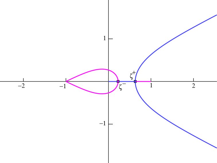
Figure 3: Steepest descent and ascent curves for $|\alpha|>1/\sqrt{2}.$ The teardrop shape and the line from $\zeta^{+}$ are both steepest descent curves, but only the contour that surrounds the origin gives a valid integral. The remainder of the lines are steepest ascent curves.

Remark: Saff and Varga show that $B(\alpha)$ is a decreasing function of $\alpha$ for $\alpha\in[1/\sqrt{2}+\varepsilon,1-\varepsilon].$ Thus the $\psi-$ functions decrease exponentially in $t$ in this range.

4.3 The transitional range: $2^{-1/2}-\varepsilon<\alpha<2^{-1/2}+\varepsilon$

We now consider the range $1/\sqrt{2}-\varepsilon<\alpha<1/\sqrt{2}+\varepsilon$. Theorems 2 and 4 exhibit an oscillating sine term times $t^{-1/2}$ for $|\alpha|<1/\sqrt{2}-\varepsilon$ and an exponentially small estimate for $|\alpha|>1/\sqrt{2}+\varepsilon.$ Saff and Varga [14] show that if $\alpha=1/\sqrt{2}$ then

$$J_{m}^{(\gamma,2\alpha/(1-\alpha)+\beta)}(0)\sim\frac{g(2\alpha-1)}{3}\left(\frac{6}{mh^{(3)}(2\alpha-1)}\right)^{1/3}e^{i\pi/3}\Gamma(1/3)$$ (88)

(See also Ambainis-et al, [3].) The asymptotic behaviour is therefore qualitatively different in the three cases $|\alpha|<1/\sqrt{2}-\varepsilon,\quad\alpha=1/\sqrt{2},$ and $\quad|\alpha|>1/\sqrt{2}+\varepsilon.$

We now apply the analysis for coalescing saddle-points as described in R. Wong’s book [16], to get a uniform asymptotic expansion for a range of $\alpha$ extending a positive distance on each side of $\alpha=1/\sqrt{2}$. The asymptotic behaviour is described in terms of the Airy function, $Ai(x).$ These functions cannot be written out explicitly, but (like Bessel functions) they can be written in terms of integral representations that are well understood. It suffices for us to know that as $x\rightarrow-\infty$ the behaviour of these functions is oscillatory,

$$Ai(-x) \sim\frac{1}{\sqrt{\pi}}\cos(\frac{2}{3}x^{3/2}-\pi/4)/x^{1/4},$$ (89)

$$Ai^{\prime}(-x) \sim\frac{x^{1/4}}{\sqrt{\pi}}\sin(\frac{2}{3}x^{3/2}-\pi/4)$$ (90)

but that when $x\rightarrow\infty$ they behave like

$$Ai(x) \sim\frac{1}{2\sqrt{\pi}}\pi x^{1/4}\exp\left(-\frac{2}{3}x^{3/2}\right),$$ (91)

$$Ai^{\prime}(x) \sim-\frac{1}{2\sqrt{\pi}}x^{1/4}\exp\left(-\frac{2}{3}x^{3/2}\right)$$ (92)

which decreases faster than any power of $x$.

Recall that we have the two saddle-points $\zeta^{-},\zeta^{+}=(\alpha\mp\sqrt{2\alpha^{2}-1})/(1+\alpha)$. Following Wong we define the variables $\zeta$ and $\eta$ by

$$\zeta^{3/2} =\frac{3}{4}(h(\zeta^{+})-h(\zeta^{-}))$$ (93)

$$\text{ or }\quad 2\zeta^{1/2}=\zeta^{+}-\zeta^{-} =2i\sqrt{1-2\alpha^{2}}/(1+\alpha),$$ (94)

$$\eta =\frac{1}{2}(h(\zeta^{-})+h(\zeta^{+}))$$ (95)

We must choose $\zeta^{-},\zeta^{+}$ as we have because we want the range of $\alpha>1/\sqrt{2}$ to give positive $\zeta$ so that there is exponential decay as $\zeta\rightarrow\infty$. Note also (as Saff and Varga point out) that if $\alpha=1/\sqrt{2}$ then

$$h^{{}^{\prime}}(\alpha) =h^{{}^{\prime\prime}}(\alpha)=0$$ (96)

$$h^{{}^{\prime\prime\prime}}(\alpha) =-\frac{1+\alpha}{24\alpha^{2}(1-\alpha)^{3}}.$$ (97)

Thus

$$h(1/\sqrt{2}+\delta)=-\frac{1+\alpha}{24\alpha^{2}(1-\alpha)^{3}}\delta^{3}+O(\delta^{4})$$ (98)

so

$$mh(\alpha)=o(1)\quad\text{ if }\quad\delta=o(m^{-1/3}).$$ (99)

Also $h(\zeta^{+})\sim h(\zeta^{-})$ so $\eta\sim h(\zeta^{-})$ for this range of $\alpha$.

Suppose for now that equation 4.31 in chapter VII of Wong [16] holds, which in our notation becomes

$$J_{m}^{(\gamma,2\alpha m/(1-\alpha)+\beta)}(0)=2\pi ie^{-m\eta}\left(\frac{Ai(m^{2/3}\zeta)}{m^{1/3}}a_{0}+\frac{Ai^{{}^{\prime}}(m^{2/3})}{m^{2/3}}b_{0}\right)(1+O(m^{-1/3}))$$ (100)

where $a_{0}$ and $b_{0}$ are independent of $m.$ (In Wong’s book, our $m$ is his $\lambda$ and our $\zeta$ is his $t.$ Our Jacobi polynomial is his $I(\lambda;\alpha),$ but his $\alpha$ is something else.) To obtain an expression for $\psi_{\rm{L}}$ we need to set $\gamma=0$ and

$$\beta=\frac{1+\alpha}{1-\alpha}$$ (101)

as in Theorem 2. Likewise, for $\psi_{\rm{R}},$ we will need to set $\gamma=1$ and

$$\beta=\frac{2\alpha}{1-\alpha}.$$ (102)

The previous argument shows that the term $m\eta=o(1)$ if $\delta=o(m^{-1/3})$ and so the $e^{m\eta}$ term is asymptotic to $1.$ Note furthermore that if $\alpha=1/\sqrt{2}+\delta$ then the definition of $\zeta$ implies that

$$\zeta=-\frac{1-2\alpha^{2}}{1+\alpha^{2}}\quad\quad=\frac{-4\sqrt{2}}{(1+\sqrt{2})^{2}}\delta+O(\delta^{2}).$$ (103)

Thus

$$m^{2/3}\zeta=-\frac{4\sqrt{2}}{(1+\sqrt{2})^{2}}m^{2/3}\delta+O(\delta^{2}).$$ (104)

When we use this estimate in the asymptotic behaviour of $Ai(m^{2/3}\zeta)$ and $Ai^{{}^{\prime}}(m^{2/3}\zeta)$ we see that the Airy functions give terms superpolynomially small if $\delta>m^{-2/3+\epsilon}.$ If $\delta=m^{-\eta},\;\eta<2/3$ however we see that the $\psi$-functions are only polynomially small. A similar argument shows that if $|\alpha|<2^{-1/2}-m^{-2/3+\epsilon}$ then the behaviour of the $\psi$ is oscillatory.

We can therefore write that the transition from oscillatory behaviour bounded below by a power of $m$ or $t$ to bounded above by a superpolynomially small function occurs when $\alpha$ varies by $O(t^{-2/3})$ from $1/\sqrt{2}$.

We may use equation 4.31 in chapter VII of Wong [16] if the transformation

$$h(\zeta)=u^{3}/3-\zeta u+\eta$$ (105)

is single-valued on the contour of integration. We may use the Gawronkski-Shawyer contour of integration (which Saff and Varga also use). The transformation will be one-to-one if on the path of integration,

$$\frac{d\zeta}{du}\neq 0\text{ and }\frac{du}{d\zeta}\neq 0.$$ (106)

Now

$$\frac{d\zeta}{du}=\frac{u^{2}-\zeta}{h^{{}^{\prime}}(\zeta)}$$ (107)

and the bottom derivative is only zero at the saddle-points. The only saddle-points are at $\zeta^{-}$ and $\zeta^{+}$. Wong shows that the choice of $\zeta^{-},\zeta^{+}$ we used implies that $\frac{d\zeta}{du}\neq 0.$ The only place the numerator is zero is at $\zeta^{-},\zeta^{+}$ and the denominator is analytic and therefore bounded on the contour of integration. We find from Wong’s book that

Theorem 5.

There is a positive $\varepsilon$ so that uniformly for some $a_{0}$ and $b_{0}$ (defined below)

$$J_{m}^{(\gamma,2\alpha m/(1-\alpha)+\beta)}(0)=2\pi ie^{-m\eta}\left(\frac{Ai(m^{2/3}\zeta)}{m^{1/3}}a_{0}+\frac{Ai^{\prime}(m^{2/3}\zeta)}{m^{2/3}}b_{0}\right)(1+O(m^{-1/3})).$$ (108)

When $n\equiv t$ mod 2 and $J_{r}^{(u,v)}(z)$ denotes a Jacobi polynomial,

$$\psi_{L}(n,t)=2^{-n/2-1}J_{m}^{(0,\frac{2\alpha m}{1-\alpha}+\frac{1+\alpha}{1-\alpha}}(0),\quad\text{ when }0\leq n<t,$$ (109)

where we can use the Remark following lemma 2 to obtain the wavefunction for negative $n.$ Also,

$$\psi_{R}(n,t)=(\frac{1+\alpha}{1-\alpha})2^{-n/2-1}J_{m}^{(1,\frac{2\alpha m}{1-\alpha}+\frac{2\alpha}{1-\alpha})}(0),\quad\text{ when }0\leq n<t,$$ (110)

and use the symmetry properties to obtain the other half as before.

So this integral representation is valid for all values of $-1+\varepsilon\leq\alpha\leq 1-\varepsilon.$ In this theorem,

$$\phi_{0}(u)=g(\zeta)\frac{d\zeta}{du}$$ (111)

and

$$a_{0} =\frac{1}{2}[\phi_{0}(\zeta^{1/2})+\phi_{0}(-\zeta^{1/2})],$$ (112)

$$b_{0} =\frac{1}{2}[\phi_{0}(\zeta^{1/2})-\phi_{0}(-\zeta^{1/2})].$$ (113)

Remark: Theorem 5 gives the asymptotic behaviour in a rather convoluted way. It is really only useful for $|\alpha|$ very near to $1/\sqrt{2},$ where the behaviour undergoes a qualitative change from oscillatory to exponential decay. For other values of $\alpha,$ Theorems 2 and 4 give much simpler expressions for the wavefunction.

Figure 4 shows the steepest descent curve when the two saddle-points coalesce.

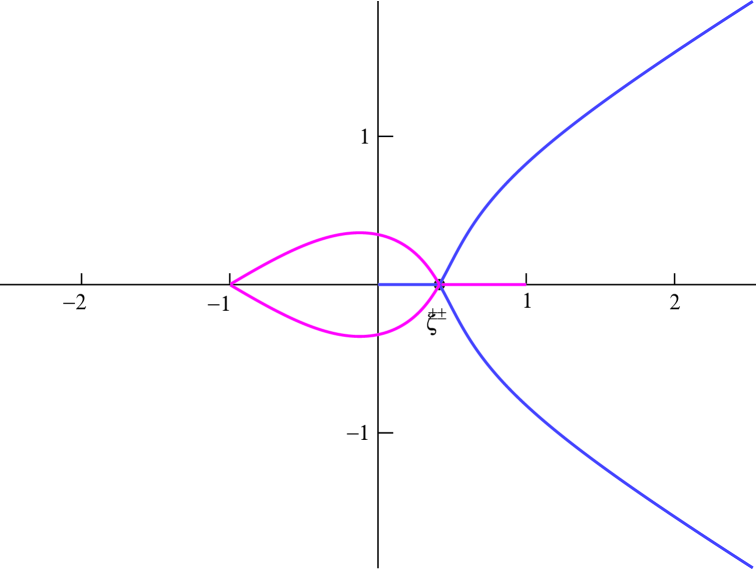
Figure 4: Steepest descent and ascent curves when the saddle-points coalesce. The tear-drop shape and the line from $\zeta^{\pm}$ comprise the steepest descent curve, and the two lines out to $\pm\infty,$ together with the line to the origin are the steepest ascent curve.

4.4 Error bounds for the method of steepest descents.

We now discuss very briefly the error-terms in our results so far. We restrict our attention to $\psi_{L}(n,t)$ and Theorem 2 above, but similar comments apply to the other results in this paper and $\psi_{R}(n,t)$. In order to apply Theorem 7.1 of Olver we expand $h(\zeta)$ and $g(\zeta)$ in powers of $\zeta-\zeta^{+}$:

$$e^{mh(\zeta)} =e^{mh(\zeta^{+})+\sum_{r=3}^{\infty}b_{r}(\zeta-\zeta^{+})^{r}}$$ (114)

$$g(\zeta) =g(\zeta^{+})+\sum_{r=1}c_{r}(\zeta-\zeta^{+})^{r}$$ (115)

and write

$$e^{\sum_{r=3}^{\infty}b_{r}(\zeta-\zeta^{+})^{r}}\left(g(\zeta^{+})+\sum_{r=1}^{\infty}c_{r}(\zeta-\zeta^{+})^{r}\right)=\sum_{s=0}^{\infty}a_{s}(\zeta-\zeta^{+})^{s}.$$ (116)

The steepest descent contour that Gawronkski and Shawyer use naturally separates into two pieces, a piece $\Gamma_{1}$ above the real axis and a piece $\Gamma_{2}$ below the real axis. Notice that $\Gamma_{1}$ is the mirror image of $\Gamma_{2}$ in the real axis. With this notation, Theorem 7.1 in Olver’s book [13] says

$$\int_{\Gamma_{1}}e^{-mh(\zeta)}g(\zeta)\sim 2e^{-mh(\zeta^{+})}\sum_{s=0}^{\infty}\Gamma(s+1/2)\frac{a_{2s}}{m^{s+1/2}}.$$ (117)

Here

$$a_{0} =\frac{g}{(2h^{\prime\prime})^{1/2}}$$ (118)

$$a_{2} =\left\{2g^{\prime\prime}-\frac{2h^{\prime\prime\prime}}{h^{\prime\prime}}+\left(\frac{5(h^{\prime\prime\prime})^{2}}{6(h^{\prime\prime})^{2}}-\frac{h^{\prime\prime\prime\prime}}{2h^{\prime\prime}}\right)g\right\}\frac{1}{(2h^{\prime\prime})^{1/2}}$$ (119)

when $g,h$ and their derivatives are evaluated at $\zeta=\zeta^{+}.$ The asymptotic expansion of the integral over $\Gamma_{2}$ is the complex conjugate of the integral over $\Gamma_{1}$. It is therefore possible to derive complete asymptotic expansions for $\psi_{\rm{L}}(n,t)$ and $\psi_{\rm{R}}(n,t)$ and certainly Gawronkski and Shawyer were aware of this. The $s=0$ term is the asymptotic formula of Theorem 2 above. Since we do not need more precision than in Theorem 2 for this application, we do not pursue this further.

Olver then explains how to derive numerical estimates for the error term. This is somewhat complicated so we refer the reader to section 10 of chapter 4 of Olver’s book. One needs to compute the maximum of certain quantities on the contour of integration. Since we do not have applications of such bounds we will not pursue that here. Olver also shows how to derive explicit numerical error bounds when the asymptotic expansion immediately above is truncated at any value of $s$.

5 The Schrödinger Approach

Nayak and Vishwanath [12] start from the recursion relations in (4) and use the Fourier transform

$$\tilde{\Psi}(k,t)=\sum_{n}\Psi(n,t)e^{ikn}$$ (120)

where $\psi(n,t)$ is defined by (1) and obtain

$$\tilde{\Psi}(k,t+1)=M_{k}\tilde{\Psi}(k,t)$$ (121)

when

$$\sqrt{2}M_{k}=\begin{pmatrix}-e^{-ik}&e^{-ik}\\ e^{ik}&e^{ik}\end{pmatrix}.$$ (122)

The eigenvalues of $M_{k}$ are

$$\lambda^{1}=e^{i\omega_{k}}, \lambda^{2}=e^{i(\pi-\omega_{k})}$$ (123)

where $\omega_{k}\in[-\pi/2,\pi/2]$ and satisfies $\sin\omega_{k}=\sin k/\sqrt{2}.$

It follows that

$$\tilde{\Psi}_{k}(t)=M_{k}^{t}\tilde{\Psi}(k,0).$$ (124)

They deduce from this that

$$\tilde{\Psi}_{\rm{L}}(k,t) =\frac{1}{2}\left(1+\frac{\cos k}{\sqrt{1+\cos^{2}k}}\right)e^{i\omega_{k}t}+\frac{(-1)^{t}}{2}\left(1-\frac{\cos k}{\sqrt{1+\cos^{2}k}}\right)e^{-i\omega_{k}t}$$ (125)

$$\tilde{\Psi}_{\rm{R}}(k,t) =\frac{e^{-ik}}{2\sqrt{1+\cos^{2}k}}\left(e^{i\omega_{k}}-(-1)^{t}e^{-\omega_{k}t}\right).$$ (126)

Formally inverting the original Fourier transform (using Cauchy’s integral formula) and some ingenious manipulations produce

$$\Psi_{\rm{L}}(n,t) =\int_{-\pi}^{\pi}\frac{dk}{2\pi}\frac{-ie^{ik}}{\sqrt{1+\cos^{2}k}}e^{-i(\omega_{k}t-kn)}$$ (127)

$$\Psi_{\rm{R}}(n,t) =\int_{-\pi}^{\pi}\frac{dk}{2\pi}\left(1+\frac{\cos k}{\sqrt{1+\cos^{2}k}}\right)e^{-i(\omega_{k}t-kn)}$$ (128)

where $\omega_{k}=\arcsin\left(\frac{\sin k}{\sqrt{2}}\right)\in[-\pi/2,\pi/2]$.

They then apply the method of stationary phase to obtain a weaker version of Theorem 2 above, and integration by parts to show that the wavefunction decays superpolynomially fast for $|\alpha|>1/\sqrt{2},$ which gives them a much weaker version of Theorem 4 (Ambainis et al. show that this decay is exponential, but they were unable to obtain uniform asymptotics). Of course both approaches consider the same functions $\Psi_{\rm{L}}(n,t)$ and $\Psi_{\rm{R}}(n,t)$, the differences are just the representation of the generating functions and the choice of contour of integration, as we will discuss below.

If $|\alpha|<\frac{1}{\sqrt{2}}$ each eigenvalue is minus the complex conjugate of the other, so the $\psi$-functions have an oscillating factor. When we find the stationary points of the phase, we obtain an equation for $k$ at the critical points, $k_{\alpha}.$ This is

$$\cos k_{\alpha}=\frac{-\alpha}{\sqrt{1-\alpha^{2}}}.$$ (129)

When $|\alpha|<1/\sqrt{2}$ this has solutions which are real and distinct. The two solutions merge at $\alpha=1/\sqrt{2},$ and then become complex. When $\alpha$ is outside the range $|\alpha|\leq 1/\sqrt{2}$ the phase has no stationary point on the real axis. We have been unable to find a method for approximating these integrals. It is worth noting that (127) are themselves integral representations of Jacobi polynomials as a function of its parameters.

The exponentially decaying solutions are counter-intuitive in other ways. As we mentioned above, for this case $k_{\alpha}$ is complex, so instead of seeing the oscillatory behaviour we might be expecting, instead the wavefunction decays within an exponential envelope. This is rather like the phenomenon of evanescent waves. These can also occur classically: consider an electromagnetic wave incident on the surface of a conductor. These waves cannot propagate in conductors, as the latter will not sustain charge gradients. However, the wave does impinge a finite distance into the conductor (the “skin depth”) over which its amplitude decays exponentially. Mathematically, this is equivalent to a complex wave-number. Evanescence can also occur in quantum mechanics, typically in regions that are classically forbidden to the particle. Strangely, both these scenarios involve the presence of some kind of barrier, but no such barrier is present for the quantum walk. These regions are not classically forbidden to the particle, it’s just very unlikely to be there.

5.1 The relationship between the two approaches

In the paper by McClure and Wong [10] the authors show that the methods of stationary phase can be reduced to the method of steepest descent under quite general conditions, as the same results can be obtained from either method, with exactly the same convergence properties. We can see this intuitively as follows. Using steepest descents, we have the integral

$$\frac{1}{2\pi i}\int_{\Gamma}g(\zeta)e^{-mh(\zeta)}\;d\zeta.$$ (130)

If the contour $\Gamma$ goes through the saddlepoint $\zeta^{+}$ we can deform $\Gamma$ to the curve $|\zeta|=|\zeta^{+}|=r$ or $\zeta=re^{i\theta},$ for some dummy variable $\theta.$ This produces an integral

$$\frac{1}{2\pi}\int_{-\pi}^{\pi}e^{-mf(re^{{i\theta}})}g(re^{i\theta})re^{i\theta}\;d\theta.$$ (131)

If we separate $f$ into its real and imaginary parts, then we obtain

$$\frac{1}{2\pi}\int_{-\pi}^{\pi}e^{-m(\Re(f(re^{i\theta}))+i\Im(f(re^{i\theta})))}g(re^{i\theta})re^{i\theta}\;d\theta.$$ (132)

For a quantum system undergoing unitary evolution, $\Re(f)=0$ and since $r$ is a constant, this integral is of the form required for the stationary phase approximation. So we will write $\mu(\theta)=\Im(f(re^{i\theta})).$

The stationary points are those $\theta$ for which $\mu(\theta)^{\prime}=0$ but since

$$\frac{d\mu(\theta)}{d\theta}=h^{\prime}(\zeta)\frac{d\zeta}{d\theta}$$ (133)

we see that the stationary points are identical to the saddle-points. With the method of steepest descents the integrand has a very small absolute value away from the saddle-point. By contrast, in the method of stationary phase the oscillations of the kernel $\mu$ become arbitrarily rapid away from the stationary point, and so self-cancel so long as $g(re^{i\theta})$ is sufficiently smooth. (Readers requiring further details are referred to the lucid exposition in [10].)

6 Conclusion

We have developed a new way of analysing the discrete quantum walk on the infinite line in terms of Airy functions, which has the advantage of being able to handle the dramatic changes in the asymptotic behaviour of this system in a uniform manner. We have also probed the mathematical relationship between the path-integral and Schrödinger approaches to solving this problem. Previous authors have found the methods of integration by parts and stationary phase to be problematic over some parts of the range of $\alpha.$ By contrast, the method of steepest descents yields a unified treatment of the system.

Acknowledgments

We are grateful to Rod Wong for drawing our attention to reference [10] and Nico Temme for kindly generating the steepest descent curves. HAC was supported by MITACS, The Fields Institute, and the NSERC CRO project “Quantum Information and Algorithms.” The research of MEHI was partially supported by NSF grant DMS 99-70865. The research of LBR was partially supported by an NSERC operating grant. We are also grateful to an anonymous referee for a very thorough reading of this paper which helped us to clarify the notation considerably.

References

• [1] Milton Abramowitz and Irene A. Stegun (Eds), Handbook of Mathematical Functions, With Formulas, Graphs, and Mathematical Tables, Dover, June 1974,   ISBN=0486612724.
• [2] Y. Aharonov, L. Davidovich, and N. Zagury, Quantum random walks, Phys. Rev. A 48 (1993), 1687.
• [3] A. Ambainis, E. Bach, A. Nayak, A. Vishwanath, and J. Watrous, One-Dimensional Quantum Walks, Proceedings of ACM Symposium on Theory of Computation (STOC’01), July 2001, Association for Computing Machinery, New York, 2001, pp. 37–49.
• [4] G. E. Andrews, R. A. Askey, and R. Roy, Special Functions, Cambridge University Press, 1999,  ISBN=0-521-62321-9.
• [5] George B. Arfken and Hans-Jurgen Weber, Mathematical Methods for Physicists, 5th ed., Academic Press, 2000,  ISBN=0-12-059825-6.
• [6] T.A. Brun, H.A. Carteret, and A. Ambainis, Quantum walks driven by many coins, 2002, quant-ph/0210161, to appear in Physical Review A.
• [7] L.-D. Chen and M. E. H. Ismail, On Asymptotics of Jacobi Polynomials, SIAM J. Math. Anal. 22 (1991), 1442–1449.
• [8] R. P. Feynman and A. R. Hibbs, Quantum Mechanics and Path Integrals, McGraw-Hill, 1965,   ISBN=0-07-020650-3.
• [9] Wolfgang Gawronkski and Bruce Shawyer, Progress in Approximation Theory, ch. Strong Asymptotics and the Limit Distribution of the Zeroes of Jacobi Polynomials $P_{n}^{an+\alpha,bn+\beta},$ ISBN=0-12-516750-4, pp. 379–404, Academic Press, 1991.
• [10] J. P. McClure and R. Wong, Justification of the stationary phase approximation in time-domain asymptotics, Proc. R. Soc. Lond. A. 453 (1997), 1019–1031.
• [11] David A. Meyer, From quantum cellular automata to quantum lattice gases, J. Stat. Phys. 85 (1996), 551–574, quant-ph/9604003.
• [12] Ashwin Nayak and Ashvin Vishwanath, Quantum Walk on the Line, 2000, quant-ph/0010117.
• [13] Frank W. J. Olver, Asymptotics and Special Functions, AKP Classics, 1997,   ISBN=1-56881-069-5.
• [14] E. B. Saff and R. S. Varga, The sharpness of Lorentz’s theorem on incomplete polynomials, Transactions of The American Mathematical Society 249 (April 1979), 163–186.
• [15] G. Szegö, Orthogonal Polynomials, 4th ed., AMS, 1975,   ISBN=0821810235.
• [16] Roderick Wong, Asymptotic Approximations of Integrals, 2nd ed., SIAM Classics in Applied Mathematics, vol. 34, Society for Industrial and Applied Mathematics, August 2001,   ISBN=0-89871-497-4.