Retrodictive states and two-photon quantum imaging

Abstract

We use retrodictive quantum theory to analyse two-photon quantum imaging systems. The formalism is particularly suitable for calculating conditional probability distributions.

1 Introduction

Two-photon quantum imaging has been studied extensively for a number of years, both experimentally and theoretically 1 . The phenomenon relies upon entanglement found in pairs of photons which are produced by spontaneous parametric down-conversion in a $\chi^{(2)}$ crystal mandel . A typical system is shown in figure 1.

Figure 1: A schematic 2-photon quantum imaging system. Arm 1 (upper) contains a mask denoted by $t$ between the crystal and the detector. This object can be imaged in arm 2.

A pump beam produces a pair of entangled photons in a type II downconversion crystal. Due to the properties of both the pump field $E_{p}$ and the nonlinear crystal (NLC) these photons are entangled in energy and wavevector. The two photons within each photon pair are emitted with polarisations orthogonal to one another, which enables their separation by means of a polarising beam splitter. After reflection or transmission at the beam splitter the photons travel on their respective paths to be detected at spatially separated detection systems. In arm 1 the photon usually propagates to a mask of some type (with transmission function $t(x)$), whose image we wish to form, and then after propagation it travels to the detector $D_{1}$, where it can be recorded at a particular position in the transverse plane. In arm 2 there is not usually any mask, simply propagation to the detector $D_{2}$. It is found that information about the object in arm 1 can be found at the detector in arm 2, even though the two paths may be widely separated, so that there is no chance that the photon in arm 2 could have interacted with the object in arm 1. Of course this can only occur when the photon in arm 1 causes the detector $D_{1}$ to fire, so the information is conditional on the occurrence of this event.

A calculation of the spatially-dependent probability distribution for joint photodetections at transverse position $x_{1}$ in arm 1 and position $x_{2}$ in arm 2, $P(x_{1},x_{2})$, can give information about the object in arm 1. The information is most directly obtained, however, from the conditional probability distribution that there is a photodetection at $x_{2}$ given that there is one at $x_{1}$, $P(x_{2}|x_{1})$. This probability distribution is what is actually produced at $D_{2}$ in a multi-shot experiment, as the detections in arm 2 are only recorded if there is also one at detector $D_{1}$. It can be found from the joint distribution using Bayes’ theorem box ,

$$P(x_{2}|x_{1})=\frac{P(x_{1},x_{2})}{P(x_{1})},$$ (1)

where of course, we assume that the arm 1 detection occurs within a small neighbourhood of $x_{1}$ in the transverse plane, and take the limit that the size of this neighbourhood tends to zero. There is redundant information in the joint probability distribution $P(x_{1},x_{2})$. It contains information, for example, about whether any photocounts are recorded by either detector due to the fact that the nonlinear crystal normally does not produce any photon pairs within a detector integration time. The conditional probability disregards this extra information, as it only deals with cases where a photon is recorded at $x_{1}$. For this reason it would be better to calculate the conditional probability directly but, as we shall see later, there is no way to do this in conventional predictive quantum mechanics.

Klyshko klyshko has suggested an advanced-wave interpretation which has proved useful for the understanding of the results of such experiments. In essence the detected state in arm 1 is thought of as evolving backwards through the system to the crystal, where a conditioning of the 2-photon state takes place, forming a 1-photon wavefunction which evolves forward in arm 2 and is imaged at the detector. The situation is similar to figure 2, which shows an unfolded version of the system. The state evolves and the light is thought of as propagating backwards through the system from the detector to the crystal. Then the state evolves forward in time as the light propagates from the crystal to the detection system in arm 2.

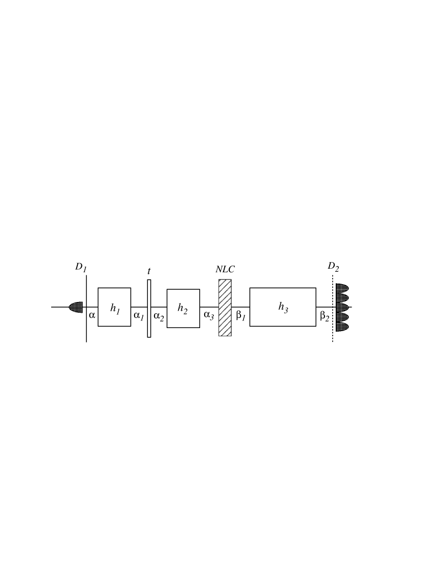
Figure 2: Unfolded version of figure 1. The state evolves from the detector on the left towards the detector on the right. The Greek letters denote the spatial functions of the 1-photon states at each point in the apparatus.

In this paper we utilise retrodictive quantum theory bayesret ; oldmaster ; newmaster , that is, quantum theory in which the state of the system at any time between preparation and measurement is assigned on the basis of a measurement performed on the final state rather than the initially prepared state, to calculate directly conditional probabilities, such as eq. (1), for quantum imaging systems. This approach has much to recommend it. Only the required probability is calculated. The redundant information in the joint distribution is not calculated because it is not useful. This is the main advantage of the retrodictive approach. Furthermore, it provides quantitative predictions based on a formal structure in which the reverse-time evolution of the measured state corresponds to Klyshko’s advanced wave interpretation. This supports the Klyshko interpretation, provides a formal derivation of conditional probabilities, and thus makes the interpretation quantitative.

The paper is organised as follows. In section 2 we describe the basic features of retrodictive quantum theory. In the following section we apply it to a general quantum imaging system such as in figure 1. We then apply the theory to a specific example. Finally we summarise our results and conclusions.

2 Retrodictive quantum theory

Quantum theory is normally formulated in a predictive manner. It is particularly useful if we wish to predict the outcomes of experiments given particular initially prepared states. Thus it provides predictive conditional probabilities. If we have a preparation device which prepares states $\hat{\rho}_{i}$ with a priori probabilities $P(i)$, and we measure these states with a device whose outputs $j$ are describable by a probability operator measure (POM) with positive elements $\hat{\Pi}_{j}$ such that $\sum_{j}\hat{\Pi}_{j}=\hat{1}$ helstrom , then the predictive conditional probability that we obtain the result $j$ if the prepared state was $\hat{\rho}_{i}$ is given by

$$P(j|i)=\mbox{Tr}\left(\hat{\rho}_{i}(t_{m})\hat{\Pi}_{j}\right)=\mbox{Tr}\left(\hat{U}(\tau)\hat{\rho}_{i}(t_{p})\hat{U}^{\dagger}(\tau)\hat{\Pi}_{j}\right),$$ (2)

where $\hat{U}$ is the unitary evolution operator which evolves the initially-prepared state from the preparation time $t_{p}$ to the measurement time $t_{m}=t_{p}+\tau$.

If we do not know which state the preparation device prepared, but only have access to the results of the measurement, then we require not the predictive but the retrodictive conditional probability $P(i|j)$. This is the probability that the state $\hat{\rho}_{i}$ was prepared given that measurement result $j$ was recorded. There are two ways in which we can calculate this probability. Either we can calculate all possible predictive conditional probabilities using predictive quantum mechanics, and then use Bayes’ theorem to find the retrodictive probability, or we can use retrodictive quantum theory bayesret ; oldmaster ; newmaster . Retrodictive quantum theory is specifically designed to give the same results as predictive quantum theory combined with Bayes’ theorem bayesret . The Bayesian approach, however, is both more calculationally intensive and less elegant than using retrodictive quantum theory.

In retrodictive quantum theory the state of a quantum system at any time between preparation and measurement is the measured state evolved backwards in time. At the preparation time the evolved measured state collapses on to the preparation basis. It has been applied to both closed systems, in which the time symmetry inherent in quantum theory simplifies calculations greatly bayesret , and to open systems, where the retrodictive state evolves backwards in time according to a retrodictive master equation analogous to the Lindblad master equation of predictive quantum theory oldmaster ; newmaster . In closed systems the retrodictive conditional probability that the prepared state was $\hat{\rho}_{i}$ given that the later measurement result is $j$ is

$$P(i|j) = \frac{\mbox{Tr}\left(P(i)\hat{\rho}_{i}\hat{\rho}_{j}(t_{p})\right)}{\sum_{k}\mbox{Tr}\left(P(k)\hat{\rho}_{k}\hat{\rho}_{j}(t_{p})\right)}$$ (3)

$$= \frac{\mbox{Tr}\left(P(i)\hat{\rho}_{i}\hat{U}^{\dagger}(\tau)\hat{\rho}_{j}(t_{m})\hat{U}(\tau)\right)}{\sum_{k}\mbox{Tr}\left(P(k)\hat{\rho}_{k}\hat{U}^{\dagger}(\tau)\hat{\rho}_{j}(t_{m})\hat{U}(\tau)\right)},$$

where the retrodictive state $\hat{\rho}_{j}(t_{m})=\hat{\Pi}_{j}/\mbox{Tr}\hat{\Pi}_{j}$ is the normalised POM element corresponding to the measurement result. This evolves backwards in time from the measurement time to the preparation time, when it collapses on to one of the states which could have been prepared.

It is clear that there is an asymmetry in the forms of the predictive and retrodictive conditional probabilities, equations (2) and (3). This is not due to any inherent time-asymmetry in quantum theory. Rather it is due to a choice in standard quantum theory to treat the predictive conditional probability as fundamental, and normalise the operators which describe prepared and measured states differently. Such a choice is not necessary, and when preparation and measurement are treated equally the predictive and retrodictive conditional probabilities take on symmetric forms prepmeas ; newmaster .

3 Retrodictive analysis

3.1 General theory

We now proceed to analyse the general system shown in figure 1. We wish to calculate the conditional probability distribution of detection at a general transverse position in arm 2 given a detection at a particular transverse position in arm 1. We will formulate the theory in one transverse dimension $x$. Extension to the whole transverse plane is straightforward.

In conventional quantum theory a fully predictive calculation is performed based on the two-photon state produced by the crystal evolved forward in time and space through both paths to form the joint probability distribution of one detection in each path. We will calculate only the conditional probability, performing a calculation which is part retrodictive and part predictive in nature, in the spirit of the Klyshko interpretation of such experiments. In order to simplify calculations further we will dispense with the formal structure of density operators and POM elements describing preparation and measurements, and simply use prepared and detected states.

Suppose that a photon is registered by a detector centred at transverse position $x_{1}$ in arm 1. This is represented by the 1-photon state

$$|1_{x}\rangle_{1}=\int dx\alpha(x)\hat{a}^{\dagger}(x)|0\rangle_{1},$$ (4)

where $\alpha(x)$ is a normalised complex function of transverse position centred on $x_{1}$, so that $\int dx|\alpha(x)|^{2}=1$. This function gives the spatial profile of the detector. The continuous-mode annihilation operator $\hat{a}(x)$ and the conjugate creation operator obey the commutator contmode

$$[\hat{a}(x),\hat{a}^{\dagger}(x^{\prime})]=\delta(x-x^{\prime}).$$ (5)

The 1-photon retrodictive state can be evolved backwards in time from the detection time. As it does so, we can follow the spatial profile back through the apparatus to the point of preparation. This approach is typical of Fourier optics fourier . We denote the various functions of $x$ at different points in the apparatus by $\alpha_{1},\alpha_{2}$ etc (fig. 2). The first part of the propagation is the propagation to the object. This is represented by convolution of the spatial detector function $\alpha(x)$ with another function of $x$, $h_{1}(x)$ to take account of the propagation. The state is still a 1-photon state, but its spatial profile has become

$$\alpha_{1}(x)=\int dx^{\prime}\alpha(x^{\prime})h_{1}(x-x^{\prime}).$$ (6)

The object which is to be imaged is accounted for by a simple transfer function $t(x)$, which is a spatially-varying complex function whose modulus is not greater than unity. Thus

$$\alpha_{2}(x)=\alpha_{1}(x)t(x).$$ (7)

Note that a one-photon wavefunction with spatial function defined by eq. (7) is not normalised. This is not a problem as we simply normalise probabilities at the end of the calculation. The next part of the propagation is from the object to the crystal. Again this is accounted for by convolution

$$\alpha_{3}(x) = \int dx^{\prime}\alpha_{2}(x^{\prime})h_{2}(x-x^{\prime})$$ (8)

$$= \int dx^{\prime}\alpha_{1}(x^{\prime})t(x^{\prime})h_{2}(x-x^{\prime})$$

$$= \int dx^{\prime}\int dx^{\prime\prime}\alpha(x^{\prime\prime})h_{1}(x^{\prime}-x^{\prime\prime})t(x^{\prime})h_{2}(x-x^{\prime}).$$

Thus the retrodictive state at the crystal is the 1-photon state of the form defined by eq. (4), but with spatial profile $\alpha$ replaced by the convolution $\alpha_{3}$.

We now condition the predictive state of the crystal using the retrodictive state from arm 1. The output of the crystal is assumed to be a 2-photon state of the form

$$|2_{x,x^{\prime}}\rangle_{1,2}=\int dx\int dx^{\prime}\beta(x,x^{\prime})\hat{a}^{\dagger}(x)\hat{b}^{\dagger}(x^{\prime})|0\rangle_{1,2},$$ (9)

where $\hat{b}^{\dagger}$ is the creation operator for arm 2. On conditioning this forms the one photon state in arm 2

$$|1_{x}\rangle_{2}=_{1}\langle 1_{x}|2_{x^{\prime},x^{\prime\prime}}\rangle_{1,2}=\int dx\beta_{1}(x)\hat{b}^{\dagger}(x)|0\rangle_{2},$$ (10)

where

$$\beta_{1}(x)=\int dx^{\prime}\alpha_{3}^{*}(x^{\prime})\beta(x^{\prime},x).$$ (11)

It is clear that by conditioning the 2-photon crystal state with the retrodictive state from the detector in arm 1 we produce a 1-photon state in arm 2. In fact the combination of the detector in arm 1 and the crystal formally constitute a quantum state preparation device prepmeas ; newmaster . The complex conjugate in this function reflects the fact that the state evolution in arm 1 has been backwards in time.

The final part of the calculation consists of propagation to the detector in arm 2. This is again taken account of by convolution with the propagation function $h_{3}(x)$. Thus

$$\beta_{2}(x)=\int dx^{\prime}\beta_{1}(x^{\prime})h_{3}(x-x^{\prime}),$$ (12)

with the state given by eq. (10) with $\beta_{2}$ as the spatial profile.

The conditional detection probability distribution for obtaining a detected photon at position $x_{2}$ in arm 2 given a detection at $x_{1}$ in arm 1, $P(x_{2}|x_{1})$ is simply given by the squared modulus of the final spatial profile, effectively a multiple spatial convolution of all of the spatial functions

$$P(x_{2}|x_{1})=\frac{\left|\beta_{2}(x_{2})\right|^{2}}{\int dx_{2}\left|\beta_{2}(x_{2})\right|^{2}}.$$ (13)

Note that we now must divide by the integral of the function in order to normalise the probability distribution. In principle we could have renormalised the 1- and 2-photon wavefunctions and this would have had the same effect.

3.2 Example: Direct imaging of an object

The utility of this general approach and of the formula derived in the previous section can be illustrated by the following simple example (see fig. 3). Suppose that there is a lens of focal length $f$ placed in each arm of the system. The pair of photons produced by the crystal is separated using a polarising beam splitter so that only one photon can be counted at each detector. The detector in arm 1 is placed at the focal length of the lens. The distance from the lens to the object to be imaged is arbitrary. We assume, however, that the object, the beam splitter and the crystal are all sufficiently close together that the small amount of propagation here has no effect, so $h_{2}(x)=1$. In arm 2 the crystal is placed at the focal length of the lens, and a spatially-resolving detector is placed after the lens. Any propagation after the lens then has no effect on the results found at the detector in arm 2.

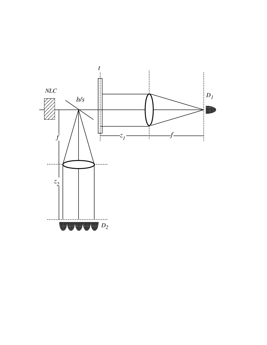
Figure 3: The system considered in section 3.1. A pair of photons produced by the crystal are separated at a polarising beam splitter (b/s) and detected at separate detection systems.

The arm 1 detector resolution function will generally be of ‘top hat’ form, but we will use a Gaussian

$$\alpha(x)=\left(\frac{1}{\pi\sigma^{2}}\right)^{1/4}e^{-(x-x_{1})^{2}/(2\sigma^{2})}$$ (14)

for ease of calculation. In any case when the spatial resolution of the detector is either very good or very poor the exact form of the function will not matter. It will be useful to write the state of the system in Fourier space

$$|1_{x}\rangle=|1_{k_{x}}\rangle=\int dk_{x}\tilde{\alpha}(k_{x})\hat{a}^{\dagger}(k_{x})|0\rangle,$$ (15)

where

$$\tilde{\alpha}(k_{x}) = \frac{1}{\sqrt{2\pi}}\int dx\alpha(x)e^{-ik_{x}x}$$ (16)

$$= \left(\frac{\sigma^{2}}{\pi}\right)^{1/4}e^{-k_{x}^{2}\sigma^{2}/2}e^{-ik_{x}x_{1}},$$ (17)

$$\hat{a}(k_{x}) = \frac{1}{\sqrt{2\pi}}\int dx\hat{a}(x)e^{-ik_{x}x}$$ (18)

are the transverse spatial Fourier transforms of the spatial function and operator, and the vacuum state is now the state of no photons at any transverse wavevector. For the Gaussian detector profile given above the detected state has a transverse wavevector profile which is also a Gaussian.

Propagation back to the lens corresponds to a modification of the transverse wavevector profile,

$$\tilde{\alpha}_{1}(k_{x})=\left(\frac{\sigma^{2}}{\pi}\right)^{1/4}e^{ifk_{z}}e^{-k_{x}^{2}\sigma^{2}/2}e^{ik_{x}^{2}f/k_{z}}e^{-ik_{x}x_{1}}.$$ (19)

The lens effectively takes the Fourier transform of this function, so that components which propagate with different transverse wavevectors between the detector and the lens all propagate with the same transverse wavevector from the lens to the object, but with spatial profile given by

$$\alpha_{1}(x) = \left(\frac{1}{\pi\sigma^{2}}\right)^{1/4}\frac{e^{ifk_{z}}}{(1-2if/k_{z}\sigma^{2})^{1/2}}$$ (20)

$$\times \exp{[-(x-x_{1})^{2}/(2\sigma^{2}(1-2if/k_{z}\sigma^{2}))]}.$$

As the spatial profile propagates unidirectionally, the distance from the lens to the object is arbitrary, and we do not consider it. After propagation back through the object the spatial profile becomes $\alpha_{2}(x)=t(x)\alpha_{1}(x)$, with $\alpha_{1}(x)$ given by eq. (20). As was stated earlier, we assume that the crystal and the polarising beam splitter are placed sufficiently close to the object that the small amount of propagation involved makes no difference. Then

$$\alpha_{3}(x)=\alpha_{2}(x)=t(x)\alpha_{1}(x).$$ (21)

The spatial profile of the 2-photon state is given by the functions

$$\tilde{\beta}(k_{x},k^{\prime}_{x}) = \sqrt{\frac{1}{2\kappa^{2}}}\exp{[-(k_{x}+k^{\prime}_{x})^{2}/2\kappa^{2}]},$$ (22)

$$\beta(x,x^{\prime}) = \sqrt{\pi}\delta(x-x^{\prime})e^{-x^{\prime 2}\kappa^{2}/2}.$$ (23)

The spread in transverse wavevector $\kappa$ of this function corresponds to the spread in transverse wavevector of the Gaussian pump beam. Phase matching then ensures that the photon pairs have wavevectors related by eq. (22). Projection of the back-propagated retrodictive 1-photon state onto this 2-photon state produced by the crystal produces a 1-photon state with profile given by eqs. (11), (21) and (23),

$$\beta_{1}(x)=\sqrt{\pi}t^{*}(x)\alpha_{1}^{*}(x)e^{-x^{2}\kappa^{2}/2},$$ (24)

and $\tilde{\beta}_{1}(k_{x})$ is found by Fourier transformation. This state, prepared by conditioning a 2-photon predictive state with a single photon retrodictive state, propagates forward in arm 2 from the crystal to the lens placed at its focal length. This propagation again corresponds to modification of $\tilde{\beta}_{1}(k_{x})$ to form

$$\tilde{\beta}_{2}(k_{x})=\tilde{\beta}_{1}(k_{x})e^{ifk_{z}}e^{ik_{x}^{2}f/k_{z}}.$$ (25)

The lens does the same as in arm 1, and effectively takes the Fourier transform of the function, giving a probability distribution which depends upon the transverse coordinate as in eq. (13). Again, any further propagation from the lens to the detector causes no change in the profile.

The result given in eq. (25) can be specialised for particular arm 1 detector profiles. In particular, for a narrow profile, given by the limit where $\sigma\rightarrow 0$. For a crystal which produces a sufficiently broad spread of wavevectors, the transverse probability distribution for detection in arm 2 takes on the form of $|t(x)|^{2}$. Thus the image of an object in arm 1 is formed at the detection system in arm 2, even though the photon in arm 2 never interacted with arm 1 at all.

The other extreme is given by a broad detector in arm 1. This gives the marginal distribution $P(x)$ which will contain no spatial information about the object in arm 1. The image is completely washed out by the broad detector.

Other propagation/detection systems in arm 2 will give a different profile. For example if the lens is placed a distance $2f$ from the crystal, and the detectors are also a distance $2f$ from the lens then for a ‘point’ detector in arm 1 the probability distribution in arm 2 is the squared modulus of the spatial fourier transform of the function $t(x)$.

4 Conclusion

In this paper we have used retrodictive quantum theory in a 2-photon quantum imaging system to calculate the conditional probability distribution for detection of a photon at a particular transverse position in one arm, given a detection at another particular position in the other arm. The retrodictive state evolves backwards in time from the detection in one arm to the nonlinear crystal, where it conditions the state of the second photon. This conditioned state then evolves forward in time in the other arm and forms the probability distribution. The approach formalises the interpretation of Klysko. We have calculated the general probability distribution as a convolution of all of the transverse spatial effects in both arm 1 and arm 2, and illustrated this with a specific example.

The advantage of the retrodictive approach over conventional predictive quantum mechanics is that only the required probability distribution is calculated. Much of the information in the full predictive probability distribution for obtaining two detections at two distinct points in the transverse plane, one in each arm is unnecessary.

In conventional quantum theory the 2-photon state is prepared by the crystal, which forms a state preparation device. The two detectors, one in each arm are measurement devices. The part-retrodictive, part-predictive approach that we have described here represents the system differently. The crystal together with the detector in arm 1 formally constitute a composite 1-photon state preparation device which prepares a photon in arm 2 whose properties are determined nonlocally in time both by physical processes in the crystal, and the later details of the propagation to the detector in arm 1.

The authors would like to thank the following bodies for financial assistance: the Overseas Research Students Awards Scheme, the University of Strathclyde, the UK Engineering and Physical Sciences Research Council, the European Commission (project QUANTIM (IST-2000-26019)), and the Australian Research Council.

References

- (1) Joobeur, A., Saleh, B.E.A. and Teich, M.C., Phys. Rev. A 50, (1994) 3349; Belinskii, A.V. and Klyshko, D.N., JETP 78, (1994) 259; Pittman, T.B., Shih, Y.H, Strekalov, D.V. and Sergienko, A.V., Phys. Rev. A 52, (1995) R3429; Joobeur, A., Saleh, B.E.A., Larchuk, T.S. and Teich, M.C., Phys. Rev. A 53, (1996) 4360; Rubin, M.H., Phys. Rev. A 54, (1996) 5349; Saleh, B.E.A., Abouraddy, A.F., Sergienko, A.V. and Teich, M.C., Phys. Rev. A 62, (2000) 043816; Abouraddy, A.F., Nasr, M.B., Saleh, B.E.A., Sergienko, A.V. and Teich, M.C., Phys. Rev. A 63, (2001) 063803; Abouraddy, A.F., Saleh, B.E.A., Sergienko, A.V. and Teich, M.C., Phys. Rev. Lett 87, (2001) 123602.
- (2) Mandel, L., and Wolf, E., Optical Coherence and Quantum Optics (Cambridge: Cambridge University Press 1995); Klyshko, D.N. Photons and Nonlinear Optics (New York: Gordon and Breach 1988).
- (3) Box, G.E.P. and Tiao, G.C., Bayesian Inference in Statistical Analysis (Sydney: Addison-Wesley 1973).
- (4) See, for example, Klyshko D.N., Sov. Phys. Usp. 31, (1988) 74.
- (5) Barnett, S.M., Pegg D.T. and Jeffers, J., J. Mod. Opt. 47, (2000) 1779, and references therein.
- (6) Barnett, S.M., Pegg, D.T., Jeffers, J. and Jedrkiewicz, O., Phys. Rev. Lett. 86, (2000) 2455.
- (7) Pegg, D.T., Barnett, S.M. and Jeffers, J., Phys. Rev. A 66, (2002) 022106.
- (8) Helstrom, C. W., Quantum Detection and Estimation Theory (Academic Press, New York 1976).
- (9) Pegg, D.T., Barnett, S.M., and Jeffers, J., J. Mod. Opt. 49, (2002) 913.
- (10) Blow, K.J., Loudon, R. Phoenix, S.J.D. and Shepherd T.J., Phys. Rev. A 42, (1990) 4102.
- (11) Goodman, J.W., Introduction to Fourier Optics (McGraw-Hill, San Francisco 1968). Abouraddy, A.F., Saleh, B.E.A., Sergienko, A.V. and Teich, M.C., J. Opt. Soc. Am. B 19, (2002) 1174.