Collisional decoherence reexamined

Abstract

We re-derive the quantum master equation for the decoherence of a massive Brownian particle due to collisions with the lighter particles from a thermal environment. Our careful treatment avoids the occurrence of squares of Dirac delta functions. It leads to a decoherence rate which is smaller by a factor of $2\pi$ compared to previous findings. This result, which is in agreement with recent experiments, is confirmed by both a physical analysis of the problem and by a perturbative calculation in the weak coupling limit.

I Introduction

A classic result of decoherence theory is the rapid decay in the off-diagonal matrix elements in the coordinate representation of the density operator $\rho(\mathbf{R}_{1},\mathbf{R}_{2};t)$ of a massive Brownian particle suffering collisions with the lighter particles of a thermal bath. Early calculations by Joos and Zeh Joos and Zeh (1985) were improved by later authors, and the result of Gallis and Fleming Gallis and Fleming (1990) seems to be the most widely quoted Giulini et al. (1996). They find, in the limit of an infinitely massive Brownian particle, that

$$\frac{\partial\rho(\mathbf{R}_{1},\mathbf{R}_{2};t)}{\partial t}=-F(\mathbf{R}_{1}-\mathbf{R}_{2})\rho(\mathbf{R}_{1},\mathbf{R}_{2};t),$$ (1)

where

$$F(\mathbf{R})=\varepsilon\,n\int_{0}^{\infty}dq\nu(q)\frac{q}{m}\int\frac{d\mathbf{\hat{n}}_{1}d\mathbf{\hat{n}}_{2}}{4\pi}\left(1-e^{iq(\mathbf{\hat{n}}_{1}-\mathbf{\hat{n}}_{2})\cdot\mathbf{R}/\hbar}\right)\left|f(q\mathbf{\hat{n}}_{2},q\mathbf{\hat{n}}_{1})\right|^{2},$$ (2)

with $m$ the mass of the bath particles, $n$ their number density, and $\nu(q)\,dq$ the fraction of particles with momentum magnitude between $q$ and $q+dq$; $\mathbf{\hat{n}}_{1}$ and $\mathbf{\hat{n}}_{2}$ are unit vectors, with $d\mathbf{\hat{n}}_{1}$ and $d\mathbf{\hat{n}}_{2}$ the elements of solid angle associated with them. The quantity $f(\mathbf{q}_{2},\mathbf{q}_{1})$ is the scattering amplitude of a bath particle off the Brownian particle from initial momentum $\mathbf{q}_{1}$ to final momentum $\mathbf{q}_{2}$. Gallis and Fleming find $\varepsilon=2\pi$.

We show here that this result is incorrect; the correct result is given by (2) with $\varepsilon=1$. Needless to say, this difference does not affect the qualitative conclusion that off-diagonal elements decay exceedingly quickly for even macroscopically small $|\mathbf{R}_{1}-\mathbf{R}_{2}|$. Nonetheless, experimental techniques are now available that permit the study of the quantum mechanical loss of coherence by collisions Hornberger et al. (2003). Therefore not only a qualitative understanding of decoherence effects is needed, but a quantitatively correct description is required as well. Moreover, derivations of benchmark equations in the theory of decoherence such (1,2) illustrate the nature of the physics and the assumptions involved, and uncovering the errors of earlier results serve as cautionary tales that may facilitate the analysis of situations where the physics is more complicated.

In this paper we present two detailed calculations of the fundamental result (1,2). The first is a scattering theory calculation in the spirit of the usual derivations, but one that avoids a pitfall of those calculations by using localized and normalized states in the scattering calculation. The second is a weak coupling calculation that follows the spirit of master equation derivations undertaken in, e.g., quantum optics. In the first calculation we find (2) with $\varepsilon=1$. In the second we find (2) with $\varepsilon=1$ and $f(q\mathbf{\hat{n}}_{2},q\mathbf{\hat{n}}_{1})$ replaced by $f_{\rm B}(q\mathbf{\hat{n}}_{2},q\mathbf{\hat{n}}_{1})$, the first Born approximation to that scattering amplitude. This is precisely what would be expected, since the second calculation requires the assumption of weak interaction; it thus serves to confirm the $\varepsilon=1$ result of the first. Neither of these is the most elegant or general calculation one could imagine; the first is rather cumbersome, and the second would be neater if generalized to second quantized form Altenmüller et al. (1997). But the first has the advantage of displaying the physics of decoherence in an almost pictorial way, while allowing a calculation involving the full scattering amplitude. And the second, in its simple form, establishes a clear connection with the usual approach to decoherence through the master equation approach common in quantum optics. Totally separate in their approaches, we feel that together they are a convincing demonstration that $\varepsilon=1$.

These two calculations are presented in sections II and IV below. In section III we return to the traditional derivation and highlight its inherent shortcomings. We show how it should be modified by using a simple physical argument, which leads to a replacement rule for the occurring square of a Dirac delta function. This treatment then also yields the result $\varepsilon=1$. Our concluding remarks are presented in section V.

II Scattering calculation

To set our notation we begin with a review of the standard approach used to calculate collisional decoherence. However, we also wish to point out the difficulties that can arise in its application, so we begin in a more detailed way than is normally done.

To apply scattering theory in a careful way one has to begin with an asymptotic-in state $\left|\phi_{m}\right\rangle\left|\psi\right\rangle$, a normalized ket that is the direct product of a Brownian particle ket $\left|\phi_{m}\right\rangle$ and a bath particle ket $\left|\psi\right\rangle$. The asymptotic-in ket is the result of the evolution of a product ket $|\phi_{m}^{(-\infty)}\rangle|\psi^{(-\infty)}\rangle$ at $t=-\infty$ to $t=0$ under the Hamiltonian that describes the free evolution of both particles, without interaction. The effect of the two-particle scattering operator $\mathcal{S}$ on this asymptotic-in state, $\mathcal{S}(|\phi_{m}\rangle|\psi\rangle)$, then produces the asymptotic-out state. When evolved from $t=0$ to $t=\infty$ by the non-interacting Hamiltonian, the asymptotic-out state yields the actual state at $t=\infty$ that evolves from $|\phi_{m}^{(-\infty)}\rangle|\psi^{(-\infty)}\rangle$ at $t=-\infty$ under the influence of the full Hamiltonian.

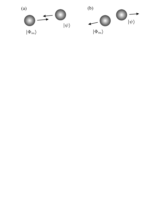
Figure 1: Sketched are the wave packets associated with $\left|\phi_{m}\right\rangle$ and $\left|\psi\right\rangle$ at $t=0$. In configuration (a) the state $\left|\phi_{m}\right\rangle\left|\psi\right\rangle$ could be taken as both an asymptotic-in state and an initial state at $t=0$; for configuration (b) that would not be possible.

In general, of course, $\left|\phi_{m}\right\rangle\left|\psi\right\rangle$ does not describe the actual ket at $t=0$ that evolves from $|\phi_{m}^{(-\infty)}\rangle|\psi^{(-\infty)}\rangle$ at $t=-\infty$, because the evolution of that actual ket involves the particle interaction. But if the kets $\left|\phi_{m}\right\rangle$ and $\left|\psi\right\rangle$ are such that the (short-range) interaction between the particles has not yet had an effect (e.g., Fig. 1a but not Fig. 1b), then $\left|\phi_{m}\right\rangle\left|\psi\right\rangle$ can be taken as the actual ket at $t=0$ as well as the asymptotic-in ket. We only consider kets $\left|\phi_{m}\right\rangle$ and $\left|\psi\right\rangle$ of this form below.

We now turn to the impending collision of a bath particle characterized by $\left|\psi\right\rangle$ and a Brownian particle described by a reduced density operator at $t=0$ given by a convex sum of projectors $|\phi_{m}\rangle\langle\phi_{m}|$,

$$\rho_{\rm in} = \sum_{m}\mathsf{p}_{m}\left|\phi_{m}\right\rangle\left\langle\phi_{m}\right|$$

$$= \int d\mathbf{R}_{1}d\mathbf{R}_{2}\;\left|\mathbf{R}_{1}\right\rangle\rho_{o}(\mathbf{R}_{1}\mathbf{,R}_{2})\left\langle\mathbf{R}_{2}\right|,$$

with probabilities $\mathsf{p}_{m}>0$, $\sum\mathsf{p}_{m}=1$. Here the $\left|\mathbf{R}_{1,2}\right\rangle$ label position eigenkets of the Brownian particle, and

$$\rho_{o}(\mathbf{R}_{1}\mathbf{,R}_{2})=\sum_{m}\mathsf{p}_{m}\left\langle\mathbf{R}_{1}\mathbf{|}\phi_{m}\right\rangle\left\langle\phi_{m}|\mathbf{R}_{2}\right\rangle$$ (3)

its position representation. Then

$$\rho_{\rm in}^{\rm total}=\rho_{\rm in}\otimes\left|\psi\right\rangle\left\langle\psi\right|$$ (4)

can be considered both as the full initial (at $t=0$) density operator, and the full asymptotic-in density operator. The full asymptotic-out density operator is then

$$\rho_{\rm out}^{\rm total} = \mathcal{S}\rho_{\rm in}^{\rm total}\mathcal{S}^{\dagger}$$

$$= \int d\mathbf{R}_{1}d\mathbf{R}_{2}\;\mathcal{S}\left(\left|\mathbf{R}_{1}\right\rangle\left|\psi\right\rangle\right)\rho_{o}(\mathbf{R}_{1}\mathbf{,R}_{2})\left(\left\langle\psi\right|\left\langle\mathbf{R}_{2}\right|\right)\mathcal{S}^{\dagger}.$$

To determine terms such as $\mathcal{S}\left(\left|\mathbf{R}\right\rangle\left|\psi\right\rangle\right)$it is useful to first consider the effect of the $\mathcal{S}$ operator on direct products $\left|\mathbf{P}\right\rangle\left|\mathbf{p}\right\rangle$ of eigenkets $\left|\mathbf{P}\right\rangle$ of the Brownian particle momentum and eigenkets $\left|\mathbf{p}\right\rangle$ of the bath particle momentum. Since the total momentum commutes with the $\mathcal{S}$ operator the scattering transformation can be reduced to a one-particle problem, with

$$\mathcal{S}\left(\left|\mathbf{P}\right\rangle\left|\mathbf{p}\right\rangle\right)=\int d\mathbf{q}\left|\mathbf{P}-\mathbf{q}\right\rangle\left|\mathbf{p+q}\right\rangle\left\langle\frac{m^{*}}{m}\mathbf{p-}\frac{m^{*}}{M}\mathbf{\mathbf{P}+q}|\mathcal{S}_{o}|\frac{m^{*}}{m}\mathbf{p-}\frac{m^{*}}{M}\mathbf{P}\right\rangle,$$

where the matrix element here is that of the one-particle scattering operator $\mathcal{S}_{o}$ corresponding to the two-body interaction acting in the Hilbert space of the bath particle, and $m^{*}=mM/(m+M)$ is the reduced mass. In the limit that the Brownian particle is much more massive than the bath particle, $M\gg m$, this reduces to

$$\mathcal{S}\left(\left|\mathbf{P}\right\rangle\left|\mathbf{p}\right\rangle\right)\rightarrow\int d\mathbf{q}\left|\mathbf{P}-\mathbf{q}\right\rangle\left|\mathbf{p+q}\right\rangle\left\langle\mathbf{p+q}|\mathcal{S}_{o}|\mathbf{p}\right\rangle$$

or, moving to a position representation for the Brownian particle,

$$\mathcal{S}\left(\left|\mathbf{R}\right\rangle\left|\mathbf{p}\right\rangle\right) = \int d\mathbf{q}\left|\mathbf{R}\right\rangle e^{-i\mathbf{q\cdot R/\hbar}}\left|\mathbf{p+q}\right\rangle\left\langle\mathbf{p+q}|\mathcal{S}_{o}|\mathbf{p}\right\rangle$$

$$= \int d\mathbf{q}\left|\mathbf{R}\right\rangle\left|\mathbf{p+q}\right\rangle\left\langle\mathbf{p+q}|e^{-i\mathcal{\mathfrak{p}\cdot}\mathbf{R}/\hbar}\mathcal{S}_{o}e^{i\mathcal{\mathfrak{p}\cdot}\mathbf{R}/\hbar}|\mathbf{p}\right\rangle$$

$$= \left|\mathbf{R}\right\rangle\left(e^{-i\mathcal{\mathfrak{p}\cdot}\mathbf{R}/\hbar}\mathcal{S}_{o}e^{i\mathcal{\mathfrak{p}\cdot}\mathbf{R}/\hbar}\left|\mathbf{p}\right\rangle\right),$$

where $\mathfrak{p}$ is the momentum operator for the bath particle, and so for general states $|\psi\rangle$

$$\mathcal{S}\left(\left|\mathbf{R}\right\rangle\left|\psi\right\rangle\right) = \left|\mathbf{R}\right\rangle\left(e^{-i\mathcal{\mathfrak{p}\cdot}\mathbf{R}/\hbar}\mathcal{S}_{o}e^{i\mathcal{\mathfrak{p}\cdot}\mathbf{R}/\hbar}\left|\psi\right\rangle\right)$$

$$\equiv \left|\mathbf{R}\right\rangle\left|\psi^{\mathbf{R}}\right\rangle,$$

where

$$\left|\psi^{\mathbf{R}}\right\rangle=e^{-i\mathcal{\mathfrak{p}\cdot}\mathbf{R}/\hbar}\mathcal{S}_{o}e^{i\mathcal{\mathfrak{p}\cdot}\mathbf{R}/\hbar}\left|\psi\right\rangle,$$

and thus

$$\rho_{\rm out}^{\rm total}=\int d\mathbf{R}_{1}d\mathbf{R}_{2}\;\left|\mathbf{R}_{1}\right\rangle\left|\psi^{\mathbf{R}_{1}}\right\rangle\rho_{o}(\mathbf{R}_{1}\mathbf{,R}_{2})\left\langle\psi^{\mathbf{R}_{2}}\right|\left\langle\mathbf{R}_{2}\right|.$$

Although $\rho_{\rm out}^{\rm total}$ is not the final density operator at $t=\infty$, but only the asymptotic-out density operator, it evolves to the final density operator through the non-interacting Hamiltonian, and overlaps of the form $\left\langle\psi^{\mathbf{R}_{2}}|\psi^{\mathbf{R}_{1}}\right\rangle$ will be preserved during this free evolution. So the final reduced density operator for the Brownian particle at $t=\infty$ is

$$\rho_{\rm final} = \int d\mathbf{R}_{1}d\mathbf{R}_{2}\;\left|\mathbf{R}_{1}\right\rangle\left\langle\psi^{\mathbf{R}_{2}}|\psi^{\mathbf{R}_{1}}\right\rangle\rho_{o}(\mathbf{R}_{1}\mathbf{,R}_{2})\left\langle\mathbf{R}_{2}\right|$$

$$\equiv \int d\mathbf{R}_{1}d\mathbf{R}_{2}\;\left|\mathbf{R}_{1}\right\rangle\rho(\mathbf{R}_{1}\mathbf{,R}_{2})\left\langle\mathbf{R}_{2}\right|,$$

where

$$\rho(\mathbf{R}_{1}\mathbf{,R}_{2})=\left\langle\psi^{\mathbf{R}_{2}}|\psi^{\mathbf{R}_{1}}\right\rangle\rho_{o}(\mathbf{R}_{1}\mathbf{,R}_{2}).$$ (5)

As is well understood, decoherence arises because the bath particle becomes entangled with the Brownian particle and the two (asymptotic-out) states $\left|\psi^{\mathbf{R}_{2}}\right\rangle$ and $\left|\psi^{\mathbf{R}_{1}}\right\rangle$ resulting from scattering interactions associated with the same bath ket $\left|\psi\right\rangle$ and different position eigenkets $\left|\mathbf{R}_{2}\right\rangle$ and $\left|\mathbf{R}_{1}\right\rangle$ can have negligible overlap even for $\left|\mathbf{R}_{2}\mathbf{-R}_{1}\right|$ small. The change of the Brownian particle’s reduced density operator by a single collision is

$$\Delta\rho(\mathbf{R}_{1}\mathbf{,R}_{2}) \equiv \rho(\mathbf{R}_{1}\mathbf{,R}_{2})-\rho_{o}(\mathbf{R}_{1}\mathbf{,R}_{2})$$ (6)

$$= \left(\left\langle\psi^{\mathbf{R}_{2}}|\psi^{\mathbf{R}_{1}}\right\rangle-1\right)\rho_{o}(\mathbf{R}_{1}\mathbf{,R}_{2})\;.$$

It involves overlap terms of the form

$$\langle\psi^{\mathbf{R}_{2}}|\psi^{\mathbf{R}_{1}}\rangle = \langle\psi|e^{-i\mathcal{\mathfrak{p}\cdot}\mathbf{R}_{2}/\hbar}\mathcal{S}_{o}^{\dagger}e^{-i\mathcal{\mathfrak{p}\cdot(}\mathbf{R}_{1}\mathbf{-R}_{2})/\hbar}\mathcal{S}_{o}e^{i\mathcal{\mathfrak{p}\cdot}\mathbf{R}_{1}/\hbar}|\psi\rangle$$ (7)

$$= \langle\psi|\mathcal{S}_{2}^{\dagger}\mathcal{S}_{1}|\psi\rangle=\mathrm{tr}_{\rm bath}\big{\{}\mathcal{S}_{2}^{\dagger}\mathcal{S}_{1}|\psi\rangle\langle\psi|\big{\}}\;,$$

where the operators

$$\mathcal{S}_{j}=e^{-i\mathcal{\mathfrak{p}\cdot}\mathbf{R}_{j}/\hbar}\mathcal{S}_{o}e^{i\mathcal{\mathfrak{p}\cdot}\mathbf{R}_{j}/\hbar}$$ (8)

for $j=1,2$ are translated scattering operators. We introduce corresponding $\mathcal{T}_{j}$ operators according to

$$\mathcal{S}_{j}=1+i\mathcal{T}_{j},$$ (9)

and using the unitarity of the $\mathcal{S}_{j}$, which follows immediately because $\mathcal{S}_{o}$ is unitary, we find

$$\mathcal{S}_{2}^{\dagger}\mathcal{S}_{1} = 1+\mathcal{T}_{2}^{\dagger}\mathcal{T}_{1}-\frac{1}{2}\mathcal{T}_{1}^{\dagger}\mathcal{T}_{1}-\frac{1}{2}\mathcal{T}_{2}^{\dagger}\mathcal{T}_{2}$$

$$+\frac{i}{2}\left(\mathcal{T}_{1}+\mathcal{T}_{1}^{\dagger}\right)-\frac{i}{2}\left(\mathcal{T}_{2}+\mathcal{T}_{2}^{\dagger}\right)$$

and so

$$\left\langle\psi^{\mathbf{R}_{2}}|\psi^{\mathbf{R}_{1}}\right\rangle=1+\left\langle\psi|\mathcal{A}|\psi\right\rangle,$$ (10)

where

$$\mathcal{A} = \mathcal{T}_{2}^{\dagger}\mathcal{T}_{1}-\frac{1}{2}\mathcal{T}_{1}^{\dagger}\mathcal{T}_{1}-\frac{1}{2}\mathcal{T}_{2}^{\dagger}\mathcal{T}_{2}$$

$$+\frac{i}{2}\left(\mathcal{T}_{1}+\mathcal{T}_{1}^{\dagger}\right)-\frac{i}{2}\left(\mathcal{T}_{2}+\mathcal{T}_{2}^{\dagger}\right).$$

Thus the change in the Brownian particle reduced density operator is

$$\Delta\rho(\mathbf{R}_{1}\mathbf{,R}_{2})=\left\langle\psi|\mathcal{A}|\psi\right\rangle\rho_{o}(\mathbf{R}_{1}\mathbf{,R}_{2})$$ (11)

The general strategy is to evaluate the matrix element $\left\langle\psi|\mathcal{A}|\psi\right\rangle$ by inserting complete sets of momentum eigenstates,

$$\left\langle\psi|\mathcal{A}|\psi\right\rangle=\int d\mathbf{q}_{1}d\mathbf{q}_{2}\left\langle\psi|\mathbf{q}_{2}\right\rangle\left\langle\mathbf{q}_{2}|\mathcal{A}|\mathbf{q}_{1}\right\rangle\left\langle\mathbf{q}_{1}|\psi\right\rangle\;,$$ (12)

determine $\left\langle\mathbf{q}_{2}|\mathcal{A}|\mathbf{q}_{1}\right\rangle$, and then perform the momentum eigenstate integrals. Writing $\mathcal{S}_{o}=1+i\mathcal{T}_{o}$ as well, and using the relations (8) and (9) we find

$$\left\langle\mathbf{q}_{2}|\mathcal{A}|\mathbf{q}_{1}\right\rangle = e^{i(\mathbf{q}_{1}\cdot\mathbf{R}_{1}-\mathbf{q}_{2}\cdot\mathbf{R}_{2})/\hbar}\left\langle\mathbf{q}_{2}|\mathcal{T}_{o}^{\dagger}e^{i\mathfrak{p}\cdot(\mathbf{R}_{2}-\mathbf{R}_{1})/\hbar}\mathcal{T}_{o}|\mathbf{q}_{1}\right\rangle$$

$$-\frac{1}{2}e^{i(\mathbf{q}_{1}-\mathbf{q}_{2})\cdot\mathbf{R}_{1}/\hbar}\left\langle\mathbf{q}_{2}|\mathcal{T}_{o}^{\dagger}\mathcal{T}_{o}|\mathbf{q}_{1}\right\rangle$$

$$-\frac{1}{2}e^{i(\mathbf{q}_{1}-\mathbf{q}_{2})\cdot\mathbf{R}_{2}/\hbar}\left\langle\mathbf{q}_{2}|\mathcal{T}_{o}^{\dagger}\mathcal{T}_{o}|\mathbf{q}_{1}\right\rangle$$

$$+\frac{i}{2}\left[e^{i(\mathbf{q}_{1}-\mathbf{q}_{2})\cdot\mathbf{R}_{1}/\hbar}-e^{i(\mathbf{q}_{1}-\mathbf{q}_{2})\cdot\mathbf{R}_{2}/\hbar}\right]\left\langle\mathbf{q}_{2}|\mathcal{T}_{o}+\mathcal{T}_{o}^{\dagger}|\mathbf{q}_{1}\right\rangle.$$

Since the $\mathcal{S}_{o}$ operator matrix elements are given by Taylor (1972)

$$\left\langle\mathbf{q}_{2}|\mathcal{S}_{o}|\mathbf{q}_{1}\right\rangle=\delta(\mathbf{q}_{2}-\mathbf{q}_{1})+\frac{i}{2\pi\hbar m}\delta(E_{2}-E_{1})f(\mathbf{q}_{2},\mathbf{q}_{1}),$$ (14)

where $f(\mathbf{q}_{2},\mathbf{q}_{1})$ is the scattering amplitude, we can identify

$$\left\langle\mathbf{q}_{2}|\mathcal{T}_{o}|\mathbf{q}_{1}\right\rangle = \frac{1}{2\pi\hbar m}\delta(E_{2}-E_{1})f(\mathbf{q}_{2},\mathbf{q}_{1})$$

$$= \frac{\delta(q_{2}-q_{1})}{2\pi\hbar q_{2}}f(\mathbf{q}_{2},\mathbf{q}_{1}),$$

where $E_{i}=q_{i}^{2}/(2m).$

Now in the traditional calculations Joos and Zeh (1985); Gallis and Fleming (1990); Giulini et al. (1996) one calculates $\partial\rho(\mathbf{R}_{1},\mathbf{R}_{2})/\partial t$ by considering the change $\Delta\rho(\mathbf{R}_{1}\mathbf{,R}_{2})$ in a time $\Delta t$ due to collisions with bath particles that would pass in the neighborhood of the Brownian particle, taking the distribution of their velocities from the assumed thermal equilibrium of the bath. To calculate $\Delta\rho(\mathbf{R}_{1}\mathbf{,R}_{2})$ from one of these bath particles, a box-normalized momentum eigenstate, $\widetilde{|\mathbf{q}\rangle}$ is used in place of a localized ket $\left|\psi\right\rangle$. Unlike the $\left|\phi_{m}\right\rangle\left|\psi\right\rangle$ states we introduced above, the $\left|\phi_{m}\right\rangle\widetilde{|\mathbf{q}\rangle}$ obviously cannot be considered either as asymptotic-in states or as the actual states at $t=0$ since the $\widetilde{|\mathbf{q}\rangle}$ are delocalized. Nonetheless, the traditional approach seems to simplify the calculation because, as is clear from (12), only diagonal elements $\left\langle\mathbf{q}|\mathcal{A}|\mathbf{q}\right\rangle$ are required if the limit of an infinite box is taken. But from the expression (II) for $\left\langle\mathbf{q}_{2}|\mathcal{A}|\mathbf{q}_{1}\right\rangle$ it is clear that, when a resolution over a complete set of momentum states $\left|\mathbf{q}^{\prime}\right\rangle$ is inserted between $\mathcal{T}_{o}^{\dagger}$ and $\mathcal{T}_{o}$ and the expression (II) for the matrix elements of $\mathcal{T}_{o}$ is used, the diagonal elements $\left\langle\mathbf{q}|\mathcal{A}|\mathbf{q}\right\rangle$ involve the square of Dirac delta functions $\delta(q-q^{\prime})$. To evaluate these the “magnitude” of $\delta(0)$ must be somehow set. This is done by relating it to an original normalization volume of the box. While not implausible, such a protocol is certainly not rigorous and is open to question.

To avoid the necessity of this kind of maneuver we will employ bath states $\left|\psi\right\rangle$ that are normalized and localized, as is required by a strict application of scattering theory. Before addressing the full calculation for a bath in thermal equilibrium we consider scattering involving a single state $\left|\psi\right\rangle$.

II.1 Scattering of a single bath ket

From the equations (12) and (II) for $\left\langle\psi|\mathcal{A}|\psi\right\rangle$ in terms of $\left\langle\mathbf{q}_{2}|\mathcal{A}|\mathbf{q}_{1}\right\rangle$ it is clear that we require integrals of the form

$$I_{1} = \int d\mathbf{q}_{1}d\mathbf{q}_{2}u(\mathbf{q}_{1},\mathbf{q}_{2})\left\langle\mathbf{q}_{2}|\mathcal{T}_{o}+\mathcal{T}_{o}^{\dagger}|\mathbf{q}_{1}\right\rangle,$$ (16)

$$I_{2}(\mathbf{R)} = \int d\mathbf{q}_{1}d\mathbf{q}_{2}u(\mathbf{q}_{1},\mathbf{q}_{2})\left\langle\mathbf{q}_{2}|\mathcal{T}_{o}^{\dagger}e^{i\mathfrak{p}\cdot\mathbf{R}/\hbar}\mathcal{T}_{o}|\mathbf{q}_{1}\right\rangle,$$

which we work out in Appendix A for an arbitrary function $u(\mathbf{q}_{1},\mathbf{q}_{2})$ of the two momentum variables. We find that we can write these expressions exactly as

$$I_{1}=\int d\mathbf{q}\int_{\mathbf{\hat{q}}^{\perp}}d\mathbf{\Delta\,}u(\mathbf{q-}\frac{\mathbf{\Delta}}{2},\mathbf{q+}\frac{\mathbf{\Delta}}{2})M_{1}(\mathbf{q,\Delta})$$ (17)

and

$$I_{2}(\mathbf{R)=}\int d\mathbf{\hat{n}\,}d\mathbf{q}\int_{\mathbf{\hat{q}}^{\perp}}d\mathbf{\Delta\,}u(\mathbf{q-}\frac{\mathbf{\Delta}}{2},\mathbf{q+}\frac{\mathbf{\Delta}}{2})e^{i\mathbf{Q\cdot R}/\hbar}M_{2}(\mathbf{q,\hat{n},\Delta),}$$ (18)

The integration over $\mathbf{q}$ covers all momentum space, while $\mathbf{\Delta}$ is a two dimensional momentum vector ranging over the plane perpendicular to $\mathbf{q}$; $\mathbf{\hat{n}}$ is a unit vector with $d\mathbf{\hat{n}}$ the associated solid angle element. Moreover,

$$M_{1}(\mathbf{q,\Delta})=\frac{1}{2\pi\hbar q}\left(f(\mathbf{q+}\frac{\mathbf{\Delta}}{2},\mathbf{q-}\frac{\mathbf{\Delta}}{2})+f^{*}(\mathbf{q-}\frac{\mathbf{\Delta}}{2},\mathbf{q+}\frac{\mathbf{\Delta}}{2})\right)$$ (19)

and

$$M_{2}(\mathbf{q,\hat{n},\Delta)=}\frac{1}{4\pi^{2}\hbar^{2}}\frac{Q}{q}f^{*}(\mathbf{Q},\mathbf{q+}\frac{\mathbf{\Delta}}{2})f(\mathbf{Q},\mathbf{q-}\frac{\mathbf{\Delta}}{2}).$$ (20)

with

$$\mathbf{Q}=\mathbf{\hat{n}}\sqrt{q^{2}+\frac{\Delta^{2}}{4}}\;.$$ (21)

With these formulas in hand we can address the expression for $\left\langle\psi|\mathcal{A}|\psi\right\rangle$ once $\left|\psi\right\rangle$ is specified. To do this, we take the bath particle wave function $\left\langle\mathbf{r}^{\prime}|\psi\right\rangle$ to be a Gaussian wave packet centered at $\mathbf{r}_{o}$ in position and $\mathbf{p}_{o}$ in momentum,

$$\left\langle\mathbf{r}^{\prime}|\psi\right\rangle=\frac{e^{i\mathbf{p}_{o}\mathbf{\cdot}\left(\mathbf{r}^{\prime}-\mathbf{r}_{o}\right)/\hbar}}{\left(\pi a^{2}\right)^{3/4}}e^{-\left|\mathbf{r}^{\prime}-\mathbf{r}_{o}\right|^{2}/(2a^{2})},$$

and characterized by

$$\Delta x = \frac{a}{\sqrt{2}},$$

$$\Delta p_{x} = \frac{b}{\sqrt{2}},$$

with $ab=\hbar$. For this minimum uncertainty wave packet we find that the expression for $\left\langle\psi|\mathbf{q}_{2}\right\rangle\left\langle\mathbf{q}_{1}|\psi\right\rangle$ in the integral (12) for $\left\langle\psi|\mathcal{A}|\psi\right\rangle$ becomes

$$\big{\langle}\psi\big{|}\mathbf{q}+\frac{\mathbf{\Delta}}{2}\big{\rangle}\big{\langle}\mathbf{q}-\frac{\mathbf{\Delta}}{2}\big{|}\psi\big{\rangle}=\left(\frac{1}{\pi b^{2}}\right)^{3/2}e^{i\mathbf{\Delta}\cdot\mathbf{r}_{o}/\hbar}e^{-\Delta^{2}/(4b^{2})}e^{-\left|\mathbf{q}-\mathbf{p}_{o}\right|^{2}/b^{2}}.$$

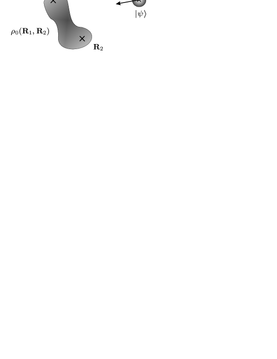
Figure 2: For this configuration the direct product of $\rho_{o}$ and $|\psi\rangle\langle\psi|$ can be taken as both the total asymptotic-in density operator and the initial density operator at $t=0$.

We now assume that this wave packet is located far enough away from the regions of space where an initial density operator (3) is concentrated, and with an average momentum directed towards the Brownian particle such that the combined density operator (4) can be taken both as an initial density operator at $t=0$, and as the asymptotic-in density operator (see Fig. 2). Then using the expressions above we find

$$\left\langle\psi|\mathcal{A}|\psi\right\rangle=\left(\frac{1}{\pi b^{2}}\right)^{3/2}\int d\mathbf{\hat{n}\,}d\mathbf{q\;}e^{-\left|\mathbf{q}-\mathbf{p}_{o}\right|^{2}/b^{2}}\int_{\mathbf{\hat{q}}^{\perp}}d\mathbf{\Delta\,}\mathcal{B}(\mathbf{\hat{n},q,\Delta)}\;,$$ (22)

where

$$\mathcal{B}(\mathbf{\hat{n},q,\Delta)} = e^{i\mathbf{q\cdot}\left(\mathbf{R}_{1}-\mathbf{R}_{2}\right)/\hbar}e^{i\mathbf{Q\cdot(R}_{2}-\mathbf{R}_{1})/\hbar}e^{-i\mathbf{\Delta\cdot(r}_{o}\mathbf{-\overline{R}})/\hbar}e^{-\Delta^{2}/(4b^{2})}M_{2}(\mathbf{q,\hat{n},\Delta)}$$

$$-\frac{1}{2}e^{-i\mathbf{\Delta\cdot(r}_{o}\mathbf{-R}_{1})/\hbar}e^{-\Delta^{2}/(4b^{2})}M_{2}(\mathbf{q,\hat{n},\Delta)}$$

$$-\frac{1}{2}e^{-i\mathbf{\Delta\cdot(r}_{o}\mathbf{-R}_{2})/\hbar}e^{-\Delta^{2}/(4b^{2})}M_{2}(\mathbf{q,\hat{n},\Delta)}$$

$$+\frac{i}{2}\left[e^{-i\mathbf{\Delta}\cdot(\mathbf{r}_{o}\mathbf{-R}_{1})/\hbar}-e^{-i\mathbf{\Delta}\cdot(\mathbf{r}_{o}\mathbf{-R}_{2})/\hbar}\right]e^{-\Delta^{2}/(4b^{2})}M_{1}(\mathbf{q,\Delta}),$$

and where we have put

$$\mathbf{\overline{R}}\equiv\frac{\mathbf{R}_{1}+\mathbf{R}_{2}}{2}.$$ (23)

The Gaussian functions will keep $\Delta$ within about $b$ of zero and $\mathbf{q}$ within about $b$ of $\mathbf{p}_{o}\mathbf{.}$ We now assume that the central momentum $\mathbf{p}_{o}$ is much greater in magnitude than its variance, $p_{o}\gg b$, and hence $q\gg b$ for all $q$ that make a significant contribution; we also assume that the scattering amplitude varies little over the momentum range $b$. Then we can put

$$M_{1}(\mathbf{q,\Delta}) \approx \frac{1}{\pi\hbar q}\mathrm{Re}\left(f(\mathbf{q},\mathbf{q})\right)$$

$$M_{2}(\mathbf{q,\hat{n},\Delta)} \approx \frac{1}{4\pi^{2}\hbar^{2}}\left|f(q\mathbf{\hat{n}},\mathbf{q})\right|^{2}.$$

Once these approximation are made the integral over $\mathbf{\Delta}$ of the three terms in $\mathcal{B}(\mathbf{\hat{n},q,\Delta)}$ can be done immediately. The integral over $\mathbf{\Delta}$ of the first term is not so simple because $\Delta$ still appears in $\mathbf{Q}$. In the exponential we have phase factors that vary as

$$\frac{\mathbf{Q\cdot(R}_{2}-\mathbf{R}_{1})}{\hbar} = \sqrt{q^{2}+\frac{\Delta^{2}}{4}}\frac{\mathbf{\hat{n}\cdot(R}_{2}-\mathbf{R}_{1})}{\hbar}$$

$$= \frac{q\mathbf{\hat{n}\cdot(R}_{2}-\mathbf{R}_{1})}{\hbar}+\frac{\Delta^{2}\mathbf{\hat{n}\cdot(R}_{2}-\mathbf{R}_{1})}{8\hbar q}+...$$

The first correction term is of order

$$\frac{b^{2}\left|\mathbf{R}_{2}-\mathbf{R}_{1}\right|}{\hbar q}=\frac{\left(\left|\mathbf{R}_{2}-\mathbf{R}_{1}\right|/a\right)}{(q/b)}$$ (24)

Since $q\gg b$ this term will still be much smaller than unity even if the distance between the two positions of the Brownian particle is several widths of the wave packet. We assume that $\left|\mathbf{R}_{2}-\mathbf{R}_{1}\right|$ is indeed such this quantity is much less than unity. Then we can replace the phase by its leading order expansion

$$\frac{\mathbf{Q\cdot(R}_{2}-\mathbf{R}_{1})}{\hbar}\approx\frac{q\mathbf{\hat{n}\cdot(R}_{2}-\mathbf{R}_{1})}{\hbar},$$

in the exponentials of the first two integrals, and the integration over $\mathbf{\Delta}$ can be done as well. These are two dimensional integrals over a plane perpendicular to $\mathbf{q}$, and so they are of the form

$$\int_{\mathbf{\hat{q}}^{\perp}}d\mathbf{\Delta}e^{-i\mathbf{\Delta\cdot(r}_{o}\mathbf{-\overline{R}})/\hbar}e^{-\Delta^{2}/(4b^{2})}=(2\pi\hbar)^{2}\Gamma_{\mathbf{q}}(\mathbf{r}_{o}\mathbf{-\overline{R})},$$

where we have used the fact that $ab=\hbar$ and introduced

$$\Gamma_{\mathbf{q}}(\mathbf{R)=}\frac{\exp\left(-\left[R^{2}-\left(\mathbf{\hat{q}\cdot R}\right)^{2}\right]/a^{2}\right)}{\pi a^{2}}$$ (25)

which involves $R^{2}-\left(\mathbf{\hat{q}\cdot R}\right)^{2}$, the square of the component of $\mathbf{R}$ that is perpendicular to $\mathbf{q}\equiv q\,\mathbf{\hat{q}}$. In all we find

$$\left\langle\psi|\mathcal{A}|\psi\right\rangle=\int d\mathbf{q}\frac{e^{-\left|\mathbf{q}-\mathbf{p}_{o}\right|^{2}/b^{2}}}{\left(\pi b^{2}\right)^{3/2}}A^{\mathbf{r}_{o}}(\mathbf{q),}$$ (26)

where

$$A^{\mathbf{r}_{o}}(\mathbf{q)} = \Gamma_{\mathbf{q}}(\mathbf{r}_{o}\mathbf{-\overline{R})}\int d\mathbf{\hat{n}\;}e^{i(\mathbf{q-}q\mathbf{\hat{n}})\mathbf{\cdot}\left(\mathbf{R}_{1}-\mathbf{R}_{2}\right)/\hbar}\left|f(q\mathbf{\hat{n}},\mathbf{q})\right|^{2}$$

$$-\frac{1}{2}\left(\Gamma_{\mathbf{q}}(\mathbf{r}_{o}\mathbf{-R}_{1})\mathbf{+}\Gamma_{\mathbf{q}}(\mathbf{r}_{o}\mathbf{-R}_{2}\mathbf{)}\right)\int d\mathbf{\hat{n}\;}\left|f(q\mathbf{\hat{n}},\mathbf{q})\right|^{2}$$

$$+\frac{2\pi i\hbar}{q}\left(\Gamma_{\mathbf{q}}(\mathbf{r}_{o}\mathbf{-R}_{1})\mathbf{-}\Gamma_{\mathbf{q}}(\mathbf{r}_{o}\mathbf{-R}_{2}\mathbf{)}\right)\mathrm{Re}\left(f(\mathbf{q},\mathbf{q})\right).$$

This is the result we will find most useful when we move to a thermal distribution of bath particles. But we close this section with an observation that is of interest in its own right. Consider the special case where the size of the bath particle wave packet is much larger than the distance between the points $\mathbf{R}_{1}$ and $\mathbf{R}_{2}$,

$$\left|\mathbf{R}_{1}-\mathbf{R}_{2}\right|/a=\left|\mathbf{R}_{1}-\mathbf{R}_{2}\right|b/\hbar\ll 1.$$ (28)

Then in the $\Gamma_{\mathbf{q}}$ functions of (II.1) we can replace $\mathbf{R}_{1}$ and $\mathbf{R}_{2}$ by $\mathbf{\overline{R}}$. Moreover, since the integral in (26) restricts $\mathbf{q}$ to within a distance of about $b$ of $\mathbf{p}_{o}$, in (II.1) we can replace $\mathbf{q}$ by $\mathbf{p}_{o}$ in the scattering amplitudes and in the phase, using the assumption already made that they vary little over a range of $b$; we can also replace the $\Gamma_{\mathbf{q}}$ functions by corresponding $\Gamma_{\mathbf{p}_{o}}$ functions. The integral in (26) can then be done, and using (11) we find

$$\Delta\rho(\mathbf{R}_{1}\mathbf{,R}_{2})=-\rho_{o}(\mathbf{R}_{1}\mathbf{,R}_{2})\Gamma_{\mathbf{p}_{o}}(\mathbf{r}_{o}\mathbf{-\overline{R})}\int d\mathbf{\hat{n}}\left(1-e^{i(\mathbf{p}_{o}-p_{o}\mathbf{\hat{n})\cdot(R}_{1}-\mathbf{R}_{2})/\hbar}\right)\left|f(p_{o}\mathbf{\hat{n}},\mathbf{p}_{o})\right|^{2}.$$

The physics here is transparent since

$$\Gamma_{\mathbf{p}_{o}}(\mathbf{r}_{o}\mathbf{-\overline{R})=}\frac{e^{-\ell^{2}/a^{2}}}{\pi a^{2}}\;,$$

where $\ell$ is the impact parameter of the collision (see Fig. 3). Decoherence occurs only if the bath particle does not “miss” the Brownian particle, i.e., if the impact parameter $\ell$ is smaller than the wave packet extension (as limited by the uncertainty principle); its maximum effect scales with the integrated square of the amplitude of the normalized bath particle as it passes over the pair of points ($1/(\pi a^{2})$); it vanishes as $\left|\mathbf{R}_{1}-\mathbf{R}_{2}\right|\rightarrow 0$ because the scattering by the two points then becomes identical; and it depends only on the scattering amplitude at momentum magnitude $p_{o}$ because the variation of that scattering amplitude over the range of momentum components included in the wave packet has been neglected.

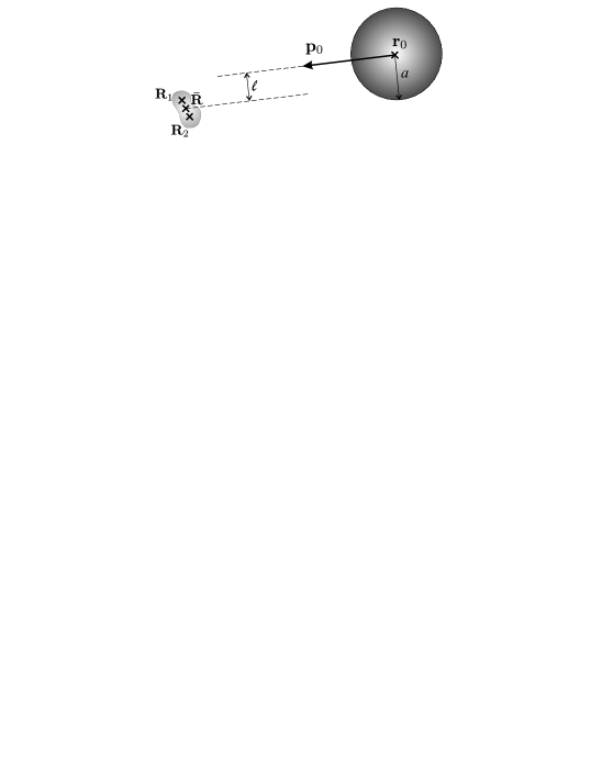
Figure 3: A configuration where $a\gg R=|\mathbf{R}_{1}-\mathbf{R}_{2}|$; $\ell=\sqrt{u^{2}-(\mathbf{u}\cdot\mathbf{\hat{p}_{o}})^{2}}$ is the impact parameter, where $\mathbf{u}=\mathbf{r}_{o}-\bar{\mathbf{R}}$.

II.2 Convex decompositions of the bath density operator

To apply the results derived above to a Brownian particle subject to a thermal bath we need to describe the effect of the thermal bath in terms of incident, normalized wave packets. We start with a single bath particle restricted to a normalization volume $\Omega$. In thermal equilibrium, at temperature $k_{B}T=\beta^{-1}$, the bath state is specified by the density operator

$$\rho^{\rm bath}=\frac{\lambda^{3}}{\Omega}e^{-\beta{\mathfrak{p}}^{2}/(2m)}$$ (29)

provided $\Omega$ is much larger than the cube of the thermal de Broglie wave length

$$\lambda=\sqrt{\frac{2\pi\hbar^{2}\beta}{m}}\;.$$ (30)

The usual convex decomposition of (29) in terms of the delocalized energy eigenstates is the obvious one and, aside from the freedom in choosing orthogonal states from among a degenerate set, it is the only one in terms of orthogonal states. But a host of others can also found. A particularly convenient set of convex decompositions for our problem at hand can be obtained by using

$$e^{-\beta{\mathfrak{p}}^{2}/(2m)}=\left(\frac{\bar{\beta}}{\beta}\right)^{3/2}\int d\mathbf{p}\,\frac{e^{-\hat{\beta}\mathbf{p}^{2}/(2m)}}{\left(2\pi m/\hat{\beta}\right)^{3/2}}\,e^{-\bar{\beta}\left(\mathfrak{p}-\mathbf{p}\right)^{2}/(2m)}$$ (31)

which holds as long as $\hat{\beta}$ and $\bar{\beta}$ are both positive and

$$\frac{1}{\beta}=\frac{1}{\bar{\beta}}+\frac{1}{\hat{\beta}}$$

or, in terms of the pseudo-temperatures $k_{\rm B}\hat{T}\equiv\hat{\beta}^{-1}$ and $k_{\rm B}\bar{T}=\bar{\beta}^{-1}$,

$$T=\bar{T}+\hat{T}.$$

In order to use the decomposition (31) for $\rho^{\rm bath}$, we write

$$e^{-\bar{\beta}\left(\mathfrak{p}-\mathbf{p}\right)^{2}/(2m)}=e^{-\bar{\beta}\left(\mathfrak{p}-\mathbf{p}\right)^{2}/(4m)}\,\mathcal{I}_{\Omega}\,e^{-\bar{\beta}\left(\mathfrak{p}-\mathbf{p}\right)^{2}/(4m)},$$

and take the identity operator in position representation

$$\mathcal{I}_{\Omega}=\int_{\Omega}d\mathbf{r}\left|\mathbf{r}\right\rangle\left\langle\mathbf{r}\right|,$$

where the integration covers the bath volume $\Omega$. We find

$$\rho^{\rm bath}=\int_{\Omega}\frac{d\mathbf{r}}{\Omega}\int d\mathbf{p}\,\hat{\mu}(\mathbf{p})\mathbf{\,}\,\left|\psi_{\mathbf{rp}}\right\rangle\left\langle\psi_{\mathbf{rp}}\right|,$$ (32)

where

$$\hat{\mu}(\mathbf{p})=\left(\frac{\hat{\beta}}{2\pi m}\right)^{3/2}e^{-\hat{\beta}\mathbf{p}^{2}/(2m)}$$ (33)

is a normalized momentum distribution function, $\int\hat{\mu}(\mathbf{p})d\mathbf{p}=1$, and the states

$$\left|\psi_{\mathbf{rp}}\right\rangle \equiv \lambda^{3/2}\left(\frac{\bar{\beta}}{\beta}\right)^{3/4}e^{-\bar{\beta}\left(\mathfrak{p}-\mathbf{p}\right)^{2}/(4m)}\left|\mathbf{r}\right\rangle$$

$$= \bar{\lambda}^{3/2}e^{-\bar{\beta}\left(\mathfrak{p}-\mathbf{p}\right)^{2}/(4m)}\left|\mathbf{r}\right\rangle,$$

are characterized by the length scale

$$\bar{\lambda}=\sqrt{\frac{2\pi\hbar^{2}\bar{\beta}}{m}}\;,$$

(compare with (30)). One then immediately finds

$$\left\langle\mathbf{r}^{\prime}|\psi_{\mathbf{rp}}\right\rangle=\frac{2\sqrt{2}}{\bar{\lambda}^{3/2}}e^{i\mathbf{p\cdot}\left(\mathbf{r}^{\prime}-\mathbf{r}\right)/\hbar}e^{-2\pi\left|\mathbf{r}^{\prime}-\mathbf{r}\right|^{2}/\bar{\lambda}^{2}}$$ (35)

so the wave packet $|\psi_{\mathbf{rp}}\rangle$ is centered at $\mathbf{r}$ and has an average momentum $\mathbf{p}$. Indeed, it is of the Gaussian form used in the preceding section with minimal uncertainties, $b\equiv\sqrt{2mk_{\rm B}\bar{T}}$ and $a\equiv\hbar/b$. Thus these wave packets have

$$\frac{\left(\Delta p_{x}\right)^{2}}{2m}=\frac{k_{\rm B}\bar{T}}{2}\;,$$

while if we calculate the momentum variance associated with the distribution function $\hat{\mu}(\mathbf{p})$,

$$\left(\delta p_{x}\right)^{2}\equiv\int p_{x}^{2}\hat{\mu}(\mathbf{p})d\mathbf{p}\;,$$

we find

$$\frac{\left(\delta p_{x}\right)^{2}}{2m}=\frac{k_{\rm B}\hat{T}}{2}\;.$$

That is,

$$\frac{\left(\Delta p_{x}\right)^{2}}{2m}+\frac{\left(\delta p_{x}\right)^{2}}{2m}=\frac{k_{\rm B}T}{2}\;.$$

We see that in the class (32,33) of convex decompositions of $\rho^{\rm bath}$ a part of the thermal kinetic energy is associated with the size of the wave packets themselves, while the rest resides in the motion of the centres of the wave packets. If we take $\hat{T}\rightarrow 0$ then the wave packets are essentially all at rest characterized by a size $\bar{\lambda}\rightarrow\lambda$, which is the thermal de Broglie wavelength. On the other hand, for $\hat{T}\gg\bar{T}$ the wave packets are much larger than the thermal de Broglie wavelength, and essentially all the thermal kinetic energy is associated with the expectation value of the momenta of the wave packets; we have

$$\frac{\left\langle\mathbf{p}^{2}\right\rangle}{2m}\equiv\frac{1}{2m}\int\mathbf{p}^{2}\hat{\mu}(\mathbf{p})d\mathbf{p=}\frac{3}{2}k_{\rm B}\hat{T},$$

and so a typical speed for the wave packets is

$$v_{\rm wp}\equiv\sqrt{\frac{3k_{\rm B}\hat{T}}{m}}.$$

II.3 Scattering of a thermal bath of particles

With the preliminaries of the preceding sections we are now in a position to begin the calculation of the effect of a thermal bath on the coherence of a massive Brownian particle. We begin with a number of assumptions and choices that will be made, and then discuss their applicability and relevance in the context of the calculation.

II.3.1 Assumptions and choices

1. We neglect initial correlations, taking the initial full density operator at $t=0$ to be a direct product of a Brownian particle density operator and a density operator for the bath particles in thermal equilibrium,

   $$\rho^{\rm total}(t=0)=\rho_{o}\otimes\rho^{\rm bath}\;.$$ (36)

2. We assume that the density of bath particles is much less than $\lambda^{-3}$; then the issue of particle degeneracy does not matter and we may consider the density operator of the total bath to be just the product of density operators for individual particles. Thus we can calculate effects ‘particle by particle’. We choose a volume $\Omega$ much larger than any other volume of interest.

3. We use a convex decomposition of $\rho^{\rm bath}$ for a single bath particle of the type described above, with $\bar{T}\ll T$ such that

   $$\hat{T}\approx T$$

   and therefore

   $$b^{2}\ll\left\langle\mathbf{p}^{2}\right\rangle\;.$$ (37)

   This renders $b$ sufficiently small so that the variation in scattering amplitudes over the momentum spread of a wave packet is negligible for essentially all of the wave packets in the convex decomposition.

4. The value of $\bar{T}$ should also be small enough that the neglect of the variation of the scattering amplitudes in the integral (22) is justified, and that we can use the approximation of neglecting terms on the order of (24) above. For the latter we need

   $$\frac{b^{2}}{\hbar q}\,|\mathbf{R}_{2}-\mathbf{R}_{1}|=\frac{2mk_{\rm B}\bar{T}}{\hbar q}\,|\mathbf{R}_{2}-\mathbf{R}_{1}|\ll 1$$

   Now for typical wave packets the average momentum $p$, and hence $q$, will be of the order of $mv_{\rm wp}=\sqrt{3mk_{\rm B}\hat{T}}$, so this condition becomes

   $$\frac{2k_{\rm B}\bar{T}}{\hbar v_{\rm wp}}\,|\mathbf{R}_{2}-\mathbf{R}_{1}|=\Big{(}\frac{8\pi}{3}\Big{)}^{1/2}\,\frac{\bar{T}}{\sqrt{T\hat{T}}}\,\frac{|\mathbf{R}_{2}-\mathbf{R}_{1}|}{\lambda}\ll 1\;,$$

   and since $\hat{T}\approx T$ this reduces to

   $$\bar{T}\ll\frac{\left|\mathbf{R}_{2}-\mathbf{R}_{1}\right|}{\lambda}\;T\;.$$

5. We choose a coarse-graining time $\Delta t$ sufficiently large that

   $$v_{\rm wp}\Delta t \gg a,$$ (38)

   $$v_{\rm wp}\Delta t \gg \left|\mathbf{R}_{2}-\mathbf{R}_{1}\right|.$$

   That is, a typical packet travels a distance much greater than its width and much greater than the distance between the two decohering sites during the coarse graining time. Using the expressions for $v_{\rm wp}$ and $a$ above, and $\hat{T}\approx T$, the first condition reads

   $$\Delta t\gg\frac{\hbar}{k_{\rm B}T}\sqrt{\frac{T}{\bar{T}}}.$$ (39)

   The second condition is essentially independent of $\bar{T}$ as long as $\hat{T}\approx T$, and simply demands that a typical bath particle wave packet can travel many times the distance between the decohering sites during the coarse-graining time.

It is easy to see that for any $\mathbf{R}_{1}$ and $\mathbf{R}_{2}$ of interest we can meet all these conditions by the choice of a large enough $\Delta t$, and we will see below that for a small enough density the change in the reduced density operator will be small over any given $\Delta t$. Hence our approximations will generally be valid in the low density limit.

II.3.2 Calculation

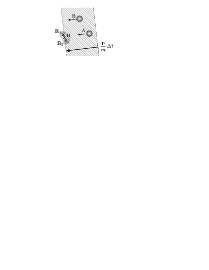
Figure 4: For wave packets with momentum $\mathbf{p}$ and centers in the hatched region $\mathsf{R}(\mathbf{p})$ we take the initial density operator to be the direct product $\rho_{o}\otimes\left|\psi_{\mathbf{rp}}\right\rangle\left\langle\psi_{\mathbf{rp}}\right|$. For some wave packets, such as (A), an actual collision will occur, while for others such as (B) one will not.

The convex decomposition (32) we use for the density operator of a bath particle leads us to think almost classically about the collision of the wave packets $|\psi_{\mathbf{rp}}\rangle$ with our Brownian particle. In a naive classical picture the bath particles of a given $\mathbf{p}$ that can be considered as coming in towards a collision with the Brownian particle in time $\Delta t$ are those that lie on any of the planes perpendicular to $\mathbf{p}$ and extending out a distance $p\Delta t/m$ in the direction $-\mathbf{\hat{p}}$ from $\mathbf{\overline{R}}$ (recall (23); see Fig. 4). Of course, some of these will completely miss the Brownian particle, but none have had a collision with it in the past. For a given $\mathbf{p}$ we refer to this region of space as $\mathsf{R}(\mathbf{p})$.

Returning to the wave packets, note that those with central positions $\mathbf{r}$ close to the $\mathbf{R}_{1}$ or $\mathbf{R}_{2}$ of interest will initially be overlapping with regions of space for which $\rho_{o}(\mathbf{R}_{1},\mathbf{R}_{2})$ is non-vanishing; here any talk of a collision is inappropriate, since at initiation, at $t=0$, the Brownian and bath particle would immediately be strongly interacting. This is an artifact of the assumption (36) of an initially uncorrelated state, which is clearly unphysical. If the uncorrelated state were taken seriously, there would be a rapid “jolt,” or shift in the reduced density operator due to the set up of correlations WeissChap2 . These effects we neglect here, as they are implicitly neglected in most such calculations; we do note that, for $\Delta t$ large enough, the regions $\mathsf{R}(\mathbf{p})$ for $\mathbf{p}$ of interest will be sufficiently large that only a small fraction of the wave packets in the sphere will fall in this problematic class.

In calculations involving the rest of the wave packets in $\mathsf{R}(\mathbf{p})$, we can take the initial density operator also to be the asymptotic-in density operator, and use the scattering theory calculation for a bath particle wave packet given above. Considering $N$ bath particles in volume $\Omega$, the total result for $\Delta\rho(\mathbf{R}_{1}\mathbf{,R}_{2})$ (recall (11) and (32)) is then

$$\Delta\rho(\mathbf{R}_{1}\mathbf{,R}_{2})=N\rho_{o}(\mathbf{R}_{1},\mathbf{R}_{2})\int d\mathbf{p\,}\hat{\mu}(\mathbf{p})\int_{\mathsf{R}(\mathbf{p})}\frac{d\mathbf{r}}{\Omega}\left\langle\psi_{\mathbf{rp}}|\mathcal{A}|\psi_{\mathbf{rp}}\right\rangle,$$

where we assume that the inclusion of the problematic class of wave packets identified above will not lead to serious error. Using the result (26) from our scattering calculation above, we have

$$\Delta\rho(\mathbf{R}_{1}\mathbf{,R}_{2})=n\rho_{o}(\mathbf{R}_{1},\mathbf{R}_{2})\int d\mathbf{p\,}\hat{\mu}(\mathbf{p})\int_{\mathsf{R}(\mathbf{p})}d\mathbf{r}\,\int d\mathbf{q}\frac{e^{-\left|\mathbf{q}-\mathbf{p}\right|^{2}/b^{2}}}{\left(\pi b^{2}\right)^{3/2}}A^{\mathbf{r}}(\mathbf{q).}$$

If in fact the strong condition (28) can be assumed then the integral over $\mathbf{q}$ can be evaluated immediately, as was done following (28), and then also the integral over $\mathbf{p}$ can be performed. But this is not necessary. We can simply note that, by virtue of (37), $\hat{\mu}(\mathbf{p})$ will vary little over the range $b$ that $e^{-\left|\mathbf{q}-\mathbf{p}\right|^{2}/b^{2}}$peaks and falls. Hence we can replace $\hat{\mu}(\mathbf{p})$ by $\hat{\mu}(\mathbf{q})$ and $\mathsf{R}(\mathbf{p})$ by $\mathsf{R}(\mathbf{q})$, and immediately do the integral over $\mathbf{p}$ to yield

$$\Delta\rho(\mathbf{R}_{1}\mathbf{,R}_{2})=n\rho_{o}(\mathbf{R}_{1},\mathbf{R}_{2})\int d\mathbf{q\,}\hat{\mu}(\mathbf{q})\int_{\mathsf{R}(\mathbf{q})}d\mathbf{r}\,A^{\mathbf{r}}(\mathbf{q).}$$

Since the only $\mathbf{r}$ dependence is in the $\Gamma_{\mathbf{q}}$, see (25), one can now do the $\mathbf{r}$ integral for each fixed $\mathbf{q}$, putting $d\mathbf{r=}d\mathbf{r}^{\bot}dr^{\|}$, where $r^{\|}$ refers to the distance in the direction $\mathbf{-q}$. Since the integration over $\mathbf{r}^{\bot}$ is unrestricted in the region $\mathsf{R}(\mathbf{q})$ we have

$$\int_{\mathsf{R}(\mathbf{q})}d\mathbf{r}^{\bot}\Gamma_{\mathbf{q}}(\mathbf{r}^{\bot}-\mathbf{R}^{\bot}_{i})=1$$

for $\mathbf{R}_{i}$ $=\mathbf{R}_{1}$, $\mathbf{R}_{2}$, or $\mathbf{\overline{R}}$, see (25). On the other hand there is no dependence on $r^{\|}$,

$$\int_{\mathsf{R}(\mathbf{q})}dr^{\|}=\frac{q}{m}\Delta t,$$

and so we find

$$\frac{\Delta\rho(\mathbf{R}_{1}\mathbf{,R}_{2})}{\Delta t}=n\rho_{o}(\mathbf{R}_{1},\mathbf{R}_{2})\int d\mathbf{q\,}\frac{q}{m}\hat{\mu}(\mathbf{q})\,\int d\mathbf{\hat{n}}\left(e^{i(\mathbf{q-}q\mathbf{\hat{n})\cdot(R}_{1}-\mathbf{R}_{2})/\hbar}-1\right)\left|f(q\mathbf{\hat{n}},\mathbf{q})\right|^{2}\;.$$

Finally, we recall that $\hat{T}\approx T$ and therefore put $\hat{\mu}(\mathbf{q})\approx\mu(\mathbf{q})$, where

$$\mu(\mathbf{q})=\left(\frac{\beta}{2\pi m}\right)^{3/2}\,e^{-\beta\mathbf{q}^{2}/(2m)}\;,$$ (40)

cf. equation (33). Now if $\nu(q)$ is the thermal distribution function for the momentum magnitude of the bath particles and $\mathbf{q}=q\mathbf{\hat{s}}$, where $\mathbf{\hat{s}}$ is a unit vector and $d\mathbf{\hat{s}}$ the associated element of solid angle, we have

$$\mu(\mathbf{q})d\mathbf{q}=\frac{\nu(q)dqd\mathbf{\hat{s}}}{4\pi},$$ (41)

and hence on a coarse grained time scale we find (1,2) with $\varepsilon=1$.

III The traditional approach: a remedy

We showed in the preceding section how the problem of evaluating a squared Dirac function can be circumvented by expressing the thermal state of the bath particles in an over-complete, non-orthogonal basis of Gaussian wave packets (see Eq. (32)). However, it is certainly reasonable to explore the possibility of using the standard diagonal representation of the thermal bath density operator, which facilitates the formal calculation considerably. After all, all the representations of $\rho^{\rm bath}$ are equally valid and should yield the same master equation provided the calculation is done in a correct way. It is therefore worthwhile to search for a way to deal properly with such an ill-defined object as the “square” of a delta distribution function.

In this section we show how a proper evaluation of the diagonal momentum basis matrix elements can be implemented. This leads to an alternate derivation of the master equation (1,2), and allows us to highlight the origin of the problem plaguing earlier workers and to discuss further implications. However, rather than attempting a mathematically rigorous formulation, we base our presentation on a simple physical argument. Our point is that such an argument can lead to a prescription for correctly evaluating improper products of Dirac delta functions, although this differs from previous naive treatments.

III.1 A single collision

Let us consider again the action of a single scattering event on the Brownian particle in position representation $\rho_{o}(\mathbf{R}_{1},\mathbf{R}_{2})$ and in the limit of a large mass. It follows from the discussion in section II that after the collision it differs merely by a factor from the initial Brownian state,

$$\rho(\mathbf{R}_{1},\mathbf{R}_{2})=\eta(\mathbf{R}_{1},\mathbf{R}_{2})\rho_{o}(\mathbf{R}_{1},\mathbf{R}_{2})$$ (42)

which is given by

$$\eta(\mathbf{R}_{1},\mathbf{R}_{2})=\mathrm{tr}_{\rm bath}\{e^{-i\mathfrak{p}\mathbf{R}_{2}/\hbar}\mathcal{S}^{\dagger}_{o}e^{i\mathfrak{p}(\mathbf{R}_{2}-\mathbf{R}_{1})/\hbar}\mathcal{S}_{o}e^{i\mathfrak{p}\mathbf{R}_{1}/\hbar}\rho^{\rm bath}\}\;,$$ (43)

(see Eqs. (5) and (7)). In section II only pure states $\rho^{\rm bath}=|\psi\rangle\langle\psi|$ of the bath particle were considered, but the reasoning is immediately generalized to mixed states.

The factor $\eta(\mathbf{R}_{1},\mathbf{R}_{2})$ may be called the decoherence function, since it describes the effective loss of coherence in the Brownian state which arises from disregarding the scattered bath particle. The normalization of $\rho^{\rm bath}$ implies

$$\lim_{|\mathbf{R}_{1}-\mathbf{R}_{2}|\to 0}\eta(\mathbf{R}_{1},\mathbf{R}_{2})=1$$ (44)

which means that the collision does not change the position distribution of the Brownian point particle, $\rho(\mathbf{R},\mathbf{R})=\rho_{o}(\mathbf{R},\mathbf{R})$. On the other hand, possible quantum correlations between increasingly far separated points will vanish, since a collision may be viewed as a position measurement of the Brownian particle by the bath which destroys superpositions of distant locations:

$$\lim_{|\mathbf{R}_{1}-\mathbf{R}_{2}|\to\infty}\eta(\mathbf{R}_{1},\mathbf{R}_{2})=0$$ (45)

This complete loss of coherence implies that the collision took place with a probability of one. It could be realized, in particular, by taking the incoming bath particle state to be a momentum eigenket in a box centered on one of the scattering sites.

In thermal equilibrium the density operator (29) of the bath particle can be written as

$$\rho^{bath} = \frac{\lambda^{3}}{\Omega}\sum_{\mathbf{p\in}\mathbb{P}_{\Omega}}e^{-\beta p^{2}/(2m)}\widetilde{\left|\mathbf{p}\right\rangle}\widetilde{\left\langle\mathbf{p}\right|}$$ (46)

$$= \frac{\left(2\pi\hbar\right)^{3}}{\Omega}\sum_{\mathbf{p\in}\mathbb{P}_{\Omega}}\mu(\mathbf{p})\,\widetilde{\left|\mathbf{p}\right\rangle}\widetilde{\left\langle\mathbf{p}\right|},$$

with the normalized momentum distribution function (40) at $\beta=1/(k_{B}T)$. The $\widetilde{\left|\mathbf{p}\right\rangle}$ are momentum eigenkets normalized with respect to the bath volume $\Omega$,

$$\widetilde{\left|\mathbf{p}\right\rangle}=\frac{\left(2\pi\hbar\right)^{3/2}}{\Omega^{1/2}}\left|\mathbf{p}\right\rangle,$$ (47)

and the sum involves those momenta $\mathbf{p\in}\mathbb{P}_{\Omega}$ whose associated wave functions satisfy periodic boundary conditions on the box $\Omega$. The kets (47) form an ortho-normal basis,

$$\sum_{\mathbf{p\in}\mathbb{P}_{\Omega}}\widetilde{\left|\mathbf{p}\right\rangle}\widetilde{\left\langle\mathbf{p}\right|}=\mathcal{I}_{\Omega}\;,$$ (48)

where $\mathcal{I}_{\Omega}$ is the identity operator in the space of wave functions which are periodic on $\Omega$; they must be distinguished from the standard momentum kets

$$\left\langle\mathbf{r|p}\right\rangle=\frac{e^{i\mathbf{p\cdot r}/\hbar}}{(2\pi\hbar)^{3/2}}\;,$$ (49)

which satisfy

$$\langle\mathbf{p|p}^{\prime}\rangle=\delta(\mathbf{p-p}^{\prime})$$

and span the full space,

$$\int d\mathbf{p}\left|\mathbf{p}\right\rangle\left\langle\mathbf{p}\right|=\mathcal{I}\text{\;.}$$ (50)

Since the bath state (46) is diagonal in the momentum representation, an explicit expression for the decoherence function (43) is readily obtained:

$$\eta(\mathbf{R}_{1},\mathbf{R}_{2}) \rightarrow \int d\mathbf{p}\,\mu(\mathbf{p})\,\widetilde{\left\langle\mathbf{p}\right|}e^{-i\mathfrak{p}\cdot\mathbf{R}_{2}/\hbar}\mathcal{S}_{o}^{\dagger}e^{i\mathfrak{p\cdot}\left(\mathbf{R}_{2}-\mathbf{R}_{1}\right)/\hbar}\mathcal{S}_{o}e^{i\mathfrak{p}\cdot\mathbf{R}_{1}/\hbar}\widetilde{\left|\mathbf{p}\right\rangle}$$ (51)

$$= \int d\mathbf{p}\,\mu(\mathbf{p})\left[1-\widetilde{\langle\mathbf{p}|}\mathcal{T}_{o}^{\dagger}\mathcal{T}_{o}\widetilde{|\mathbf{p}\rangle}+e^{i\mathbf{p}\cdot(\mathbf{R}_{1}-\mathbf{R}_{2})/\hbar}\widetilde{\langle\mathbf{p}|}\mathcal{T}_{o}^{\dagger}e^{i\mathfrak{p}\cdot(\mathbf{R}_{2}-\mathbf{R}_{1})/\hbar}\mathcal{T}_{o}\widetilde{|\mathbf{p}\rangle}\right]$$

$$= \int d\mathbf{p}\,\mu(\mathbf{p})\left[1-\frac{(2\pi\hbar)^{3}}{\Omega}\int d\mathbf{p}^{\prime}\left(1-e^{i\left(\mathbf{p-p}^{\prime}\right)\cdot\left(\mathbf{R}_{1}-\mathbf{R}_{2}\right)/\hbar}\right)\left|\left\langle\mathbf{p}^{\prime}|\mathcal{T}_{o}|\mathbf{p}\right\rangle\right|^{2}\right]$$

In the first line the sum over momenta $\mathbf{p\in}\mathbb{P}_{\Omega}$ was replaced by an integral according to the usual prescription

$$\frac{\left(2\pi\hbar\right)^{3}}{\Omega}\sum_{\mathbf{p\in}\mathbb{P}_{\Omega}}\;\rightarrow\;\int d\mathbf{p}\;.$$

In the second line we introduced the operator $\mathcal{T}_{o}=i(1-\mathcal{S}_{o})$ and used the unitarity of $\mathcal{S}_{o}$,

$$i(\mathcal{T}_{o}-\mathcal{T}_{o}^{\dagger})=-\mathcal{T}_{o}^{\dagger}\mathcal{T}_{o}\;,$$

as in section II and in Gallis and Fleming (1990); Giulini et al. (1996). The last line follows after inserting a complete set of states (50) and noting the relation (47).

The expression in square brackets in (51) should be well-defined and finite. However, it involves two arbitrarily large quantities, the “quantization volume” $\Omega$, which stems from the normalization of the bath particle, and the squared amplitude of the $\mathcal{T}_{o}$-operator with respect to (improper) momentum kets. The simple matrix element is given by the expression (II)

$$\langle\mathbf{p}^{\prime}|\mathcal{T}_{o}|\mathbf{p}\rangle=\frac{\delta(p-p^{\prime})}{2\pi\hbar p}\,f(\mathbf{p}^{\prime},\mathbf{p})$$ (52)

involving the scattering amplitude and a delta-function which ensures the conservation of energy during an elastic collision. The squared modulus of (52) is not well defined in the sense of distributions, but depends on the specific limiting process from which the Dirac delta function originates. Yet one would naturally expect that an appropriate replacement has the form

$$\big{|}\langle\mathbf{p}^{\prime}|\mathcal{T}_{o}|\mathbf{p}\rangle\big{|}^{2}\to\delta(p-p^{\prime})\,g(\mathbf{p})\,\big{|}f(\mathbf{p}^{\prime},\mathbf{p})\big{|}^{2}$$ (53)

with $g(\mathbf{p})$ a function involving the quantization volume.

We note that (51) displays the correct limiting behavior (44) since the expression in round brackets vanishes as $\mathbf{R}_{1}\to\mathbf{R}_{2}$. On the other hand, for large separations of the points the phase in (51) oscillates rapidly and it will not contribute to the integral in the limit $|\mathbf{R}_{1}-\mathbf{R}_{2}|\to\infty$. Therefore the limit (45) allows to specify the unknown function $g(\mathbf{p})$ in (53). One obtains

$$g(\mathbf{p})=\frac{\Omega}{(2\pi\hbar)^{3}}\,\frac{1}{\sigma(\mathbf{p})p^{2}}$$

with

$$\sigma(\mathbf{p})=\int d\mathbf{\hat{n}}\,\big{|}f(p\,\mathbf{\hat{n}},\mathbf{p})\big{|}^{2}$$

the total cross section for scattering at momentum $\mathbf{p}$. Formally, this means that one should treat the expression involving the squared $\delta$-function and scattering amplitude as

$$\big{|}\delta(p-p^{\prime})f(p^{\prime}\mathbf{\hat{n}},\mathbf{p})\big{|}^{2}\to\frac{\Omega}{2\pi\hbar\sigma(\mathbf{p})}\,\delta(p-p^{\prime})\,\big{|}f(p\,\mathbf{\hat{n}},\mathbf{p})\big{|}^{2}\;.$$ (54)

III.2 The master equation

A master equation can now be derived in the same spirit as above. In the low density limit for the bath particles, the decohering effect of each collision can be treated independently and the overall decoherence in a short time interval $\Delta t$ is determined only by the mean number and type of single collisions.

For bath particles with momentum $\mathbf{p}$ the mean number of collisions is given by $j(\mathbf{p})\sigma(\mathbf{p})\Delta t$, where $j(\mathbf{p})=n|\mathbf{p}|/m$ is the flux, and we replace $1/\Omega$ by $n$, the number density of bath particles. Hence, the average change in the Brownian state during $\Delta t$ reads

$$\frac{\rho(\mathbf{R}_{1},\mathbf{R}_{2})-\rho_{o}(\mathbf{R}_{1},\mathbf{R}_{2})}{\Delta t}=-n\int d\mathbf{p}\,\mu(\mathbf{p})\frac{p}{m}\int d\mathbf{\hat{n}}\big{(}1-e^{i(\mathbf{p}-p\,\mathbf{\hat{n}})(\mathbf{R}_{1}-\mathbf{R}_{2})/\hbar}\big{)}$$

$$\times\big{|}f(p\,\mathbf{\hat{n}},\mathbf{p})\big{|}^{2}\rho_{o}(\mathbf{R}_{1},\mathbf{R}_{2})$$

and noting (41) we have on a coarse-grained time scale which is much larger than the typical interval between collisions

$$\frac{\partial}{\partial t}\rho(\mathbf{R}_{1},\mathbf{R}_{2})=-F(\mathbf{R}_{1}-\mathbf{R}_{2})\rho(\mathbf{R}_{1},\mathbf{R}_{2})\;.$$ (55)

with $F$ given by (2), again with $\varepsilon=1$.

III.3 Interpretation

It is clear that the derivation of the decoherence function (43) does not hold rigorously even for volume-normalized (47) momentum states, since their amplitude is uniform in space and they cannot be considered as asymptotic-in or asymptotic-out states. Nonetheless, the fact that one obtains the “correct” master equation by using the diagonal momentum representation (46) indicates that it can be reasonable, at least in a formal sense, to extend the applicability of (43) to volume-normalized momentum eigenstates.

Then the appearance of the total cross section in the appropriate replacement rule (54) has a clear physical interpretation. The squared matrix element of the $\mathcal{T}_{o}$ operator with respect to two orthogonal proper states may be viewed as the probability for a transition between the states due to a collision. The appropriate normalization of the probability necessary in the limit of improper states is then effected by the appearance of the total cross section $\sigma(\mathbf{p})$ in (54), which is absent in the usual naive treatments of the squared delta function.

This point of view is confirmed by the fact that the rule (54), which was derived from a simple physical argument (45), implies a conservation condition. Integrating (54) we have

$$\frac{(2\pi\hbar)^{3}}{\Omega}\int d\mathbf{p}^{\prime}\big{|}\langle\mathbf{p}^{\prime}|\mathcal{T}_{o}|\mathbf{p}\rangle\big{|}^{2}\to\int d\mathbf{p}^{\prime}\delta(p-p^{\prime})\,\,\frac{\big{|}f(\mathbf{p}^{\prime},\mathbf{p})\big{|}^{2}}{p^{2}\,\sigma(\mathbf{p})}=1$$ (56)

and hence, using (50) and switching to volume-normalized states,

$$\widetilde{\langle\mathbf{p}|}\mathcal{T}_{o}\mathcal{T}_{o}^{\dagger}\widetilde{|\mathbf{p}\rangle}\to 1\;.$$ (57)

Inserting the identity (48) yields

$$\sum_{\mathbf{p}^{\prime}\in\mathbb{P}_{\Omega}}\big{|}\widetilde{\langle\mathbf{p}^{\prime}|}\mathcal{T}_{o}\widetilde{|\mathbf{p}\rangle}\big{|}^{2}\to 1\;.$$ (58)

This is reminiscent of the situation of a multi-junction in mesoscopic physics Imry1997a , or of the scattering off a quantum graph Kottos2003a , where one defines a transition matrix $\mathsf{T}_{mn}=|t_{mn}|^{2}$ which connects a finite number of incoming and outgoing channels. There the $t_{mn}$ are the transmission amplitudes between the incoming and outgoing states and the current conservation implies

$$\sum_{m}\mathsf{T}_{mn}=1\quad\quad\mbox{with}\quad\quad\mathsf{T}_{mn}=|t_{mn}|^{2}\;,$$

in analogy to (58).

The fact that the conservation relation (58) has no meaningful equivalence in the continuum limit $\Omega\to\infty$ is closely connected to the difficulty of evaluating the squared scattering amplitude in the momentum representation. It suggests that the diagonal representation of $\rho^{\rm bath}$ can be used in a rigorous formulation of the master equation only if the transition of going from a discrete to a continuous set of bath states is delayed until after the square of the scattering matrix element is evaluated. A calculation along this line, albeit in a perturbative framework, is presented in the following section.

IV Weak-coupling calculation

We now consider an approach that is totally different from the derivation in Section II. Instead of performing a scattering calculation, we obtain a master equation for the reduced density operator from a weak coupling approximation that is very similar to the analyses of quantum optics. Again the assumption of a low density of bath particles will allow us to calculate the effect of the bath particles one particle at a time, so we begin with our Brownian particle and a single bath particle restricted to a box of normalization volume $\Omega$. While we will take the limit $\Omega\rightarrow\infty$ in the course of the calculation, we can do it in such a way that products of Dirac delta functions never appear.

In the absence of any interaction between the particles the Hamiltonian reads

$$H_{o}=\frac{\mathcal{P}^{2}}{2M}+\frac{\mathfrak{p}^{2}}{2m},$$

where $m$ and $M$ are the bath and Brownian particle masses and $\mathfrak{p}$ and $\mathcal{P}$ are their momentum operators. The normalized eigenstates of $H_{o}$ are direct products $\widetilde{|\mathbf{{P}}\rangle}\widetilde{|\mathbf{{p}}\rangle}$, where $\widetilde{|\mathbf{{p}}\rangle}$ is given by (47) with (49), and similarly

$$\langle\mathbf{R\widetilde{|{P}}\rangle}=\frac{e^{i\mathbf{{P}\cdot R}/\hbar}}{\sqrt{\Omega}}\;.$$ (59)

The values of $\mathbf{{p}}$ and $\mathbf{{P}}$ are restricted to a discrete set, $\mathbf{{p}},\mathbf{{P}}\in\mathbb{P}_{\Omega}$, so that the wave functions respect periodic boundary conditions. Our full Hamiltonian is then

$$H=H_{o}+V(\mathfrak{r-}\mathcal{R}),$$

where $\mathfrak{r}$ and $\mathcal{R}$ are respectively the bath and Brownian particle position operators, and $V$ describes the interaction.

In the interaction picture the full density operator evolves according to

$$\rho_{I}^{\rm total}(t)=U(t)\rho_{I}^{\rm total}(0)U^{\dagger}(t),$$ (60)

where $U(t)=1+iT(t),$ and

$$T(t)=-\frac{1}{\hbar}\int_{0}^{t}H_{I}(t^{\prime})U(t^{\prime})dt^{\prime},$$

with

$$H_{I}(t)=e^{iH_{o}t/\hbar}V(\mathfrak{r-}\mathcal{R})e^{-iH_{o}t/\hbar}.$$ (61)

Using the unitarity of the time evolution, $U^{\dagger}(t)U(t)=U(t)U^{\dagger}(t)=\mathcal{I}$, we find from (60) and the definition of $T(t)$ that

$$\rho_{I}^{\rm total}(t)-\rho_{I}^{\rm total}(0) = \frac{1}{2}i\left[T(t)+T^{\dagger}(t),\rho_{I}^{\rm total}(0)\right]$$

$$+T(t)\rho_{I}^{\rm total}(0)T^{\dagger}(t)-\frac{1}{2}T^{\dagger}(t)T(t)\rho_{I}^{\rm total}(0)-\frac{1}{2}\rho_{I}^{\rm total}(0)T^{\dagger}(t)T(t).$$

This equation is exact. The first term on the right side describes a unitary modification to the dynamics of the density operator due to the interaction with the bath particles; we neglect it here since it will not lead to decoherence. For the other terms we make the standard weak-coupling approximations Gardiner and Zoller (2000): we replace $T(t)$ by

$$T_{o}=-\frac{1}{\hbar}\int_{0}^{\Delta t}H_{I}(t^{\prime})dt^{\prime},$$

assume an initially uncorrelated density operator, $\rho_{I}^{\rm total}(0)=\rho_{o}\otimes\rho^{\rm bath}$, (cf. equation (36)), and at time $\Delta t$ trace over the bath to find the change in the reduced density operator for the Brownian particle as

$$\Delta\rho_{I}=\mathrm{tr}_{\rm bath}\big{\{}T_{o}\rho_{o}\rho^{\rm bath}T_{o}^{\dagger}-\frac{1}{2}T_{o}^{\dagger}T_{o}\rho_{o}\rho^{\rm bath}-\frac{1}{2}\rho_{o}\rho^{\rm bath}T_{o}^{\dagger}T_{o}\big{\}}.$$ (62)

To construct $T_{o}$ we begin with a Fourier expansion of the interaction potential, writing

$$V(\mathfrak{r-}\mathcal{R})=\frac{\left(2\pi\hbar\right)^{3}}{\Omega}\sum_{\mathbf{{q}}\in\mathbb{P}_{\Omega}}\bar{V}(\mathbf{{q}})e^{i\mathbf{{q}}\cdot\left(\mathfrak{r-}\mathcal{R}\right)/\hbar},$$ (63)

choosing the prefactor for later convenience. Then forming (61), by inserting resolutions of unity (48) in terms of the energy eigenstates between the free evolution terms and the potential, we find

$$H_{I}(t) = \frac{\left(2\pi\hbar\right)^{3}}{\Omega}\sum_{\mathbf{{P}},\mathbf{{q}}\in\mathbb{P}_{\Omega}}\bar{V}(\mathbf{{q}})\widetilde{|{\mathbf{P}-\mathbf{q}}\rangle}\widetilde{\langle\mathbf{{P}}|}\exp\left(\frac{it}{\hbar}\frac{\left|{\mathbf{P}-\mathbf{q}}\right|^{2}-{P}^{2}}{2M}\right)$$ (64)

$$\times\sum_{\mathbf{{p}}\in\mathbb{P}_{\Omega}}\widetilde{|{\mathbf{p}+\mathbf{q}}\rangle}\widetilde{\langle\mathbf{{p}}|}\exp\left(\frac{it}{\hbar}\frac{\left|{\mathbf{p}+\mathbf{q}}\right|^{2}-{p}^{2}}{2m}\right).$$

Although this approach leads easily to considering the more general problem of a finite mass Brownian particle, we defer that to a later communication. Here we take the infinite mass limit for the Brownian particle by taking $M\rightarrow\infty$ in (64), and we can then write

$$H_{I}(t)=\frac{\left(2\pi\hbar\right)^{3}}{\Omega}\sum_{\mathbf{{P},{q}}\in\mathbb{P}_{\Omega}}\tilde{\Lambda}_{\mathbf{{P}{q}}}\gamma_{\mathbf{{q}}}(t),$$

where

$$\tilde{\Lambda}_{\mathbf{{P}{q}}}=\widetilde{|{\mathbf{P}-\mathbf{q}}\rangle}\widetilde{\langle\mathbf{{P}}|}$$

and

$$\gamma_{\mathbf{{q}}}(t)=\bar{V}(\mathbf{{q}})\sum_{\mathbf{{p}}\in\mathbb{P}_{\Omega}}\widetilde{|{\mathbf{p}+\mathbf{q}}\rangle}\widetilde{\langle\mathbf{{p}}|}\exp\left(\frac{it}{\hbar}\frac{\left|{\mathbf{p}+\mathbf{q}}\right|^{2}-{p}^{2}}{2m}\right).$$

Using these in the expression (62) for $\Delta\rho$, we find

$$\Delta\rho = \frac{\left(2\pi\hbar\right)^{6}}{\Omega^{2}}\sum_{\mathbf{{P}}^{\prime},\mathbf{{q}}^{\prime},\mathbf{{P}}^{\prime\prime},\mathbf{{q}}^{\prime\prime}\in\mathbb{P}_{\Omega}}\left(2\tilde{\Lambda}_{\mathbf{{P}}^{\prime}\mathbf{{q}}^{\prime}}\rho_{o}\tilde{\Lambda}_{\mathbf{{P}}^{\prime\prime}\mathbf{{q}}^{\prime\prime}}^{\dagger}-\tilde{\Lambda}_{\mathbf{{P}}^{\prime\prime}\mathbf{{q}}^{\prime\prime}}^{\dagger}\tilde{\Lambda}_{\mathbf{{P}}^{\prime}\mathbf{{q}}^{\prime}}\rho_{o}-\rho_{o}\tilde{\Lambda}_{\mathbf{{P}}^{\prime\prime}\mathbf{{q}}^{\prime\prime}}^{\dagger}\tilde{\Lambda}_{\mathbf{{P}}^{\prime}\mathbf{{q}}^{\prime}}\right)\Upsilon(\mathbf{{q}}^{\prime},\mathbf{{q}}^{\prime\prime}),$$

with

$$\Upsilon(\mathbf{{q}}^{\prime},\mathbf{{q}}^{\prime\prime})=\frac{1}{2\hbar^{2}}\int_{0}^{\Delta t}\int_{0}^{\Delta t}\mathrm{tr}_{\rm bath}\big{\{}\gamma_{\mathbf{{q}}^{\prime}}(t^{\prime})\rho^{\rm bath}\gamma_{\mathbf{{q}}^{\prime\prime}}^{\dagger}(t^{\prime\prime})\big{\}}\,dt^{\prime}dt^{\prime\prime}\;.$$

Here we no longer distinguish between the Schrödinger and the interaction picture of the reduced density operator since they yield the same evolution in the infinite mass limit. The response function $\Upsilon(\mathbf{{q}}^{\prime},\mathbf{{q}}^{\prime\prime})$ involves the correlator

$$\mathrm{tr}_{\rm bath}\big{\{}\gamma_{\mathbf{{q}}^{\prime}}(t^{\prime})\rho^{\rm bath}\gamma_{\mathbf{{q}}^{\prime\prime}}^{\dagger}(t^{\prime\prime})\big{\}}=\delta_{\mathbf{{q}}^{\prime}\mathbf{{q}}^{\prime\prime}}\left|\bar{V}(\mathbf{{q}}^{\prime})\right|^{2}\sum_{\mathbf{{p}}\in\mathbb{P}_{\Omega}}N_{\mathbf{{p}}}\exp\left(\frac{i(t^{\prime}-t^{\prime\prime})}{\hbar}\left(\frac{\left|{\mathbf{p}+\mathbf{q}^{\prime}}\right|^{2}-{p}^{2}}{2m}\right)\right)$$

where

$$N_{\mathbf{{p}}}=\widetilde{\langle\mathbf{{p}}|}\rho^{\rm bath}\widetilde{|\mathbf{{p}}\rangle}$$

is the probability associated with state $\widetilde{|\mathbf{{p}}\rangle}$. At this point we include the fact that $N$ particles exist in volume $\Omega$ by multiplying the one particle probability by $N$. Moreover, for a large volume $\Omega$ we can replace the summation over the bath momenta by an integral,

$$\sum_{\mathbf{{p}}\in\mathbb{P}_{\Omega}}\frac{N_{\mathbf{{p}}}}{\Omega}\,\ldots\;\rightarrow\;\int d\mathbf{p}\,n\mu(\mathbf{p})\ldots\;,$$

where $n$ is the bath particle density and $\mu(\mathbf{p})$ the thermal distribution function (40). This yields

$$\mathrm{tr}_{\rm bath}\big{\{}\gamma_{\mathbf{{q}}^{\prime}}(t^{\prime})\rho^{\rm bath}\gamma_{\mathbf{{q}}^{\prime\prime}}^{\dagger}(t^{\prime\prime})\big{\}} = \delta_{\mathbf{{q}}^{\prime}\mathbf{{q}}^{\prime\prime}}\Omega\left|\bar{V}(\mathbf{{q}}^{\prime})\right|^{2}\int n\mu(\mathbf{p})\exp\left(\frac{i(t^{\prime}-t^{\prime\prime})}{\hbar}\left(\frac{\left|\mathbf{p}+\mathbf{{q}}^{\prime}\right|^{2}-p^{2}}{2m}\right)\right)d\mathbf{p}$$ (65)

$$\equiv \delta_{\mathbf{{q}}^{\prime}\mathbf{{q}}^{\prime\prime}}\Omega G_{\mathbf{{q}}^{\prime}}(t^{\prime\prime}-t^{\prime}),$$

with

$$G_{\mathbf{q}}(t^{\prime\prime}-t^{\prime})=n\left|\bar{V}(\mathbf{q})\right|^{2}\int\mu(\mathbf{p})\exp\left(\frac{i(t^{\prime}-t^{\prime\prime})}{\hbar}\left(\frac{\left|\mathbf{p}+\mathbf{q}\right|^{2}-p^{2}}{2m}\right)\right)d\mathbf{p}$$ (66)

for all $\mathbf{q}$. Then we have

$$\Delta\rho=\frac{\left(2\pi\hbar\right)^{6}}{\Omega^{2}}\frac{\Omega}{2\hbar^{2}}\sum_{\mathbf{{P}}^{\prime},\mathbf{{P}}^{\prime\prime},\mathbf{{q}}\in\mathbb{P}_{\Omega}}\left(2\tilde{\Lambda}_{\mathbf{{P}}^{\prime}\mathbf{{q}}}\rho_{o}\tilde{\Lambda}_{\mathbf{{P}}^{\prime\prime}\mathbf{{q}}}^{\dagger}-\tilde{\Lambda}_{\mathbf{{P}}^{\prime\prime}\mathbf{{q}}}^{\dagger}\tilde{\Lambda}_{\mathbf{{P}}^{\prime}\mathbf{{q}}}\rho_{o}-\rho_{o}\tilde{\Lambda}_{\mathbf{{P}}^{\prime\prime}\mathbf{{q}}}^{\dagger}\tilde{\Lambda}_{\mathbf{\tilde{P}}^{\prime}\mathbf{{q}}}\right)I_{\mathbf{{q}}}(\Delta t).$$ (67)

where

$$I_{\mathbf{q}}(\Delta t)\equiv\int_{0}^{\Delta t}\int_{0}^{\Delta t}G_{\mathbf{q}}(t^{\prime\prime}-t^{\prime})\,dt^{\prime}dt^{\prime\prime}\;.$$

Now that the Kronecker delta appearing in (65) has been summed we can pass to the continuum limit $\Omega\to\infty$ and switch from the box-normalized states (59) to the standard momentum kets for the Brownian particle,

$$\left\langle\mathbf{R|P}\right\rangle = \frac{e^{i\mathbf{P\cdot R}/\hbar}}{\sqrt{(2\pi\hbar)^{3}}}\;.$$

This is done by the replacements

$$\frac{\Omega}{(2\pi\hbar)^{3}}\,\tilde{\Lambda}_{\mathbf{{P}}\mathbf{{q}}}\;\rightarrow\;\left|\mathbf{P-q}\right\rangle\left\langle\mathbf{P}\right|\equiv\Lambda_{\mathbf{P}\mathbf{q}}$$

and

$$\frac{(2\pi\hbar)^{3}}{\Omega}\sum_{\mathbf{{P}}\in\mathbb{P}_{\Omega}}\;\rightarrow\;\int d\mathbf{{P}}\;.$$ (68)

We obtain

$$\frac{\Delta\rho}{4\pi^{3}\hbar}=\int d\mathbf{P}^{\prime}d\mathbf{P}^{\prime\prime}d\mathbf{q}\left(2\Lambda_{\mathbf{P}^{\prime}\mathbf{q}}\rho_{o}\Lambda_{\mathbf{P}^{\prime\prime}\mathbf{q}}^{\dagger}-\Lambda_{\mathbf{P}^{\prime\prime}\mathbf{q}}^{\dagger}\Lambda_{\mathbf{P}^{\prime}\mathbf{q}}\rho_{o}-\rho_{o}\Lambda_{\mathbf{P}^{\prime\prime}\mathbf{q}}^{\dagger}\Lambda_{\mathbf{P}^{\prime}\mathbf{q}}\right)I_{\mathbf{q}}(\Delta t)\;.$$

Similarly, the Fourier transform of (63) yields in the limit (68)

$$\bar{V}(\mathbf{q}) = \int\frac{d\mathbf{r}}{\left(2\pi\hbar\right)^{3}}V(\mathbf{r})e^{-i\mathbf{q\cdot r}/\hbar}$$

$$= \left\langle\mathbf{q}|V|\mathbf{0}\right\rangle$$

as the momentum matrix element of the interaction.

By means of the Fourier expansion

$$G_{\mathbf{q}}(t)=\int\frac{d\omega}{2\pi}\bar{G}_{\mathbf{q}}(\omega)e^{-i\omega t}$$ (69)

we can write

$$I_{\mathbf{q}}(\Delta t)=\frac{1}{2\pi}\int d\omega\bar{G}_{\mathbf{q}}(\omega)\left[\frac{\sin\left(\omega\Delta t/2\right)}{\omega/2}\right]^{2},$$

where

$$\bar{G}_{\mathbf{q}}(\omega)=\frac{2\pi nm\hbar}{q}\left|\bar{V}(\mathbf{q})\right|^{2}\left(\frac{\beta}{2\pi m}\right)^{1/2}\exp\left[-\frac{\beta m\hbar^{2}}{2q^{2}}\left(\omega-\frac{q^{2}}{2m\hbar}\right)^{2}\right],$$ (70)

as we show in Appendix B. It follows that for time intervals

$$\Delta t\gg\beta\hbar$$ (71)

we can set $\bar{G}_{\mathbf{q}}(\omega)\approx\bar{G}_{\mathbf{q}}(0)$, and $I_{\mathbf{q}}(\Delta t)\approx\bar{G}_{\mathbf{q}}(0)\Delta t$ for essentially all $\mathbf{q}$ of importance in (67); a coarse graining time long enough that (71) is satisfied is sufficient to guarantee that Fermi’s Golden Rule holds and energy conservation is satisfied for the scattering bath particles. We then obtain a master equation for the reduced density operator of the Brownian particle,

$$\frac{d\rho}{dt}=4\pi^{3}\hbar\int d\mathbf{P}^{\prime}d\mathbf{P}^{\prime\prime}d\mathbf{q\,}\left(2\Lambda_{\mathbf{P}^{\prime}\mathbf{q}}\rho\Lambda_{\mathbf{P}^{\prime\prime}\mathbf{q}}^{\dagger}-\Lambda_{\mathbf{P}^{\prime\prime}\mathbf{q}}^{\dagger}\Lambda_{\mathbf{P}^{\prime}\mathbf{q}}\rho-\rho\Lambda_{\mathbf{P}^{\prime\prime}\mathbf{q}}^{\dagger}\Lambda_{\mathbf{P}^{\prime}\mathbf{q}}\right)\bar{G}_{\mathbf{q}}(0).$$

Although not explicitly in Lindblad form this equation yields a completely positive evolution of $\rho$ and can be put in Lindblad form, since $\bar{G}_{\mathbf{q}}(0)>0$.

To see the physics of this result and to compare it with earlier work we go into the coordinate representation, $\rho(\mathbf{R}_{1},\mathbf{R}_{2};t)=\left\langle\mathbf{R}_{1}|\rho(t)|\mathbf{R}_{2}\right\rangle$, were we find

$$\frac{d\rho(\mathbf{R}_{1},\mathbf{R}_{2};t)}{dt}=-F(\mathbf{R}_{1}-\mathbf{R}_{2})\rho(\mathbf{R}_{1},\mathbf{R}_{2};t),$$

with

$$F(\mathbf{R})=8\pi^{3}\hbar\int d\mathbf{q}\left(1-e^{-i\mathbf{q\cdot R}/\hbar}\right)\bar{G}_{\mathbf{q}}(0).$$ (72)

While this in practice might be a useful expression for evaluating $F(\mathbf{R})$ directly, to compare with earlier work it is easiest to return first to (66) and formally determine $\bar{G}_{\mathbf{q}}(0)$. Inserting in (72) leads to

$$F(\mathbf{R})=16\pi^{4}\hbar^{2}n\int d\mathbf{q}\int d\mathbf{p}\,\mu(\mathbf{p})\left|\bar{V}(\mathbf{q})\right|^{2}\left[1-e^{-i\mathbf{q\cdot R}/\hbar}\right]\delta\left(\frac{\left|\mathbf{p}+\mathbf{q}\right|^{2}-p^{2}}{2m}\right),$$

and with the introduction of a new variable $\mathbf{p}^{\prime}=\mathbf{p+q}$ to replace $\mathbf{q}$,

$$F(\mathbf{R})=16\pi^{4}\hbar^{2}n\int\int d\mathbf{p}^{\prime}d\mathbf{p}\,\mu(\mathbf{p})\left|\bar{V}(\mathbf{p}^{\prime}-\mathbf{p})\right|^{2}\left[1-e^{i(\mathbf{p-p}^{\prime})\mathbf{\cdot R}/\hbar}\right]\delta\left(\frac{\left(p^{\prime}\right)^{2}-p^{2}}{2m}\right).$$

The $\mathbf{p}^{\prime}$ integration can be done in polar coordinates, $\mathbf{p}^{\prime}=p^{\prime}\mathbf{\hat{n}}$, i.e, $d\mathbf{p}^{\prime}=(p^{\prime})^{2}dp^{\prime}d\mathbf{\hat{n}}$. Then since

$$\delta\Big{(}\frac{\left(p^{\prime}\right)^{2}-p^{2}}{2m}\Big{)}=\delta\Big{(}\frac{p^{\prime}+p}{2m}(p^{\prime}-p)\Big{)}=\frac{m}{p}\,\delta(p^{\prime}-p),$$

we have

$$F(\mathbf{R})=16\pi^{4}\hbar^{2}nm\int\int d\mathbf{\hat{n}}d\mathbf{p}\mu(\mathbf{p})p\left|\bar{V}(p\mathbf{\hat{n}}-\mathbf{p})\right|^{2}\left[1-e^{i(\mathbf{p-}p\mathbf{\hat{n}})\mathbf{\cdot R}/\hbar}\right],$$

which, with the aid of (41), yields

$$F(\mathbf{R)}=4\pi^{3}\hbar^{2}mn\int\int p\nu(p)dp\,d\mathbf{\hat{n}\,}d\mathbf{\hat{s}}\left|\bar{V}(p\mathbf{\hat{n}}-p\mathbf{\hat{s}})\right|^{2}\left[1-e^{i(p\mathbf{\hat{s}-}p\mathbf{\hat{n}})\mathbf{\cdot R}/\hbar}\right].$$

Finally, we use the fact that the first order Born approximation for the scattering amplitude is given by Taylor (1972)

$$f_{\rm B}(\mathbf{p}^{\prime},\mathbf{p)}=-(2\pi)^{2}m\hbar\bar{V}(\mathbf{p}^{\prime}-\mathbf{p)}$$ (73)

to find

$$F(\mathbf{R})=n\int\int\frac{p}{m}\nu(p)dp\frac{\,d\mathbf{\hat{n}\,}d\mathbf{\hat{s}}}{4\pi}\left|f_{B}(p\mathbf{\hat{n},}p\mathbf{\hat{s})}\right|^{2}\left[1-e^{i(p\mathbf{\hat{s}-}p\mathbf{\hat{n}})\mathbf{\cdot R}/\hbar}\right],$$

in agreement with (2) for $\varepsilon=1$, if the full scattering amplitude is replaced by its first Born approximation.

V Conclusions

In this article we presented two detailed derivations of the quantum master equation for a massive Brownian particle subject to collisions with particles from a thermalized environment, and a third argument for the master equation based on physical motivations. They represent rather different strategies of dealing with the principal problem that arises in the formulation of collisional decoherence: The momentum eigenstates that are the most natural for describing the density operator of the thermal bath do not constitute proper states for the application of scattering theory.

By representing the thermal bath with an appropriate over-complete basis, we obtained in section II the full master equation in a calculation that is mathematically and physically convincing, but cumbersome. The perturbative treatment in section  IV permitted the avoidance of improper states up to a point where they could be handled in an unambiguous way. Yet this calculation hides some of the physics involved, and does not in itself suggest an immediate generalization to higher orders in the perturbation parameter. More straightforward, but also most ventured, is the use of the replacement rule put forward in section  III. It yields the master equation immediately, but lacks the mathematical foundation one would wish for an equation describing a process as fundamental as decoherence by collisions. The strategies developed here lead to natural generalizations, both to the more general problem of a Brownian particle of finite mass, and to other collisional decoherence processes. We plan to turn to them in future communications.

Different as the three approaches may be, they all suggest that previous results in the literature predict decoherence rates that are quantitatively too large. This conclusion is not only of theoretical interest. A recent experiment Hornberger et al. (2003) on the decoherence of fullerene matter waves by collisions with background gas atoms was sensitive to the presence or absence of the factor of $2\pi$ that has been the focus of this article. And indeed, the observed decoherence rates are in full agreement with the equation derived in this article, and exclude the previous results.

Appendix A

In this Appendix we confirm the results (17,18), beginning from the definitions (16). We begin by inserting a complete set of momentum eigenstates to write the matrix element appearing in $I_{2}(\mathbf{R})$ as

$$\left\langle\mathbf{q}_{2}|\mathcal{T}_{o}^{\dagger}e^{i\mathfrak{p}\cdot\mathbf{R}/\hbar}\mathcal{T}_{o}|\mathbf{q}_{1}\right\rangle = \int d\mathbf{q}^{\prime}\left\langle\mathbf{q}_{2}|\mathcal{T}_{o}^{\dagger}e^{i\mathfrak{p}\cdot\mathbf{R}/\hbar}|\mathbf{q}^{\prime}\right\rangle\left\langle\mathbf{q}^{\prime}|\mathcal{T}_{o}|\mathbf{q}_{1}\right\rangle$$

$$= \int d\mathbf{q}^{\prime}e^{i\mathbf{q}^{\prime}\cdot\mathbf{R}/\hbar}\left\langle\mathbf{q}_{2}|\mathcal{T}_{o}^{\dagger}|\mathbf{q}^{\prime}\right\rangle\left\langle\mathbf{q}^{\prime}|\mathcal{T}_{o}|\mathbf{q}_{1}\right\rangle.$$

Then using the expression (II) for the matrix elements of $\mathcal{T}_{o}$ and, noting that we can write $\delta(q_{2}-q^{\prime})\delta(q^{\prime}-q_{1})=\delta(q_{2}-q_{1})\delta(q^{\prime}-q_{1})$, we find

$$I_{1} = \int\frac{d\mathbf{q}_{1}d\mathbf{q}_{2}}{2\pi\hbar q_{2}}u(\mathbf{q}_{1},\mathbf{q}_{2})\left(f(\mathbf{q}_{2},\mathbf{q}_{1})+f^{*}(\mathbf{q}_{1},\mathbf{q}_{2})\right)\delta(q_{2}-q_{1}),$$ (74)

$$I_{2}(\mathbf{R}) = \int\frac{d\mathbf{q}_{1}d\mathbf{q}_{2}d\mathbf{q}^{\prime}}{4\pi^{2}\hbar^{2}q_{1}q_{2}}u(\mathbf{q}_{1},\mathbf{q}_{2})e^{i\mathbf{q}^{\prime}\cdot\mathbf{R}/\hbar}f^{*}(\mathbf{q}^{\prime},\mathbf{q}_{2})f(\mathbf{q}^{\prime},\mathbf{q}_{1})\delta(q^{\prime}-q_{1})\delta(q_{2}-q_{1}),$$

and so $\delta(q_{2}-q_{1})$ appears in both these expressions. They are simplified if we make a change of variables from $(\mathbf{q}_{1},\mathbf{q}_{2})$ to $(\mathbf{q},\mathbf{s})$, where $\mathbf{q}_{2}=\mathbf{q+}{\mathbf{s}}/{2}$ and $\mathbf{q}_{1}=\mathbf{q-}{\mathbf{s}}/{2}$. The Jacobian of this transformation is unity, so $d\mathbf{q}_{1}d\mathbf{q}_{2}=d\mathbf{q}d\mathbf{s}$, and

$$\delta(q_{2}-q_{1})=\delta\left(\sqrt{q^{2}+\frac{s^{2}}{4}+\mathbf{s\cdot q}}-\sqrt{q^{2}+\frac{s^{2}}{4}-\mathbf{s\cdot q}}\right).$$

We do the $\mathbf{s}$ integral first, and we single out the component of $\mathbf{s}$ along $\mathbf{\hat{q}}$ by writing

$$\mathbf{s=}\nu\mathbf{\hat{q}+\Delta},$$

where $\mathbf{\Delta}$ is a two-dimensional vector lying in the plane perpendicular to $\mathbf{\hat{q}}$. Then $d\mathbf{s}=d\nu d\mathbf{\Delta}$, and

$$\delta(q_{2}-q_{1})=\delta(g(\nu))$$

for fixed $\mathbf{\Delta}$, where

$$g(\nu)=\sqrt{q^{2}+\frac{\Delta^{2}+\nu^{2}}{4}+q\nu}-\sqrt{q^{2}+\frac{\Delta^{2}+\nu^{2}}{4}-q\nu}$$

which as a function of $\nu$ vanishes at $\nu=0$. Thus

$$\delta(g(\nu))=\frac{\delta(\nu)}{\left|dg/d\nu\right|_{\nu=0}}=\frac{\sqrt{q^{2}+\frac{\Delta^{2}}{4}}}{q}\delta(\nu)\;,$$

and for any function $U(\mathbf{q}_{1},\mathbf{q}_{2})$ we have

$$d\mathbf{q}_{1}d\mathbf{q}_{2}U(\mathbf{q}_{1},\mathbf{q}_{2})\delta(q_{2}-q_{1})$$

$$= d\mathbf{q}d\nu d\mathbf{\Delta\,}U(\mathbf{q}-\frac{\mathbf{s}}{2},\mathbf{q}+\frac{\mathbf{s}}{2})\delta(g(\nu))$$

$$= d\mathbf{q}d\mathbf{\Delta}\frac{Q}{q}\mathcal{\,}U(\mathbf{q}-\frac{\mathbf{\Delta}}{2},\mathbf{q}+\frac{\mathbf{\Delta}}{2})\;,$$

where we have put

$$Q\equiv\sqrt{q^{2}+\frac{\Delta^{2}}{4}}=\left|\mathbf{q-}\frac{\mathbf{\Delta}}{2}\right|=\left|\mathbf{q+}\frac{\mathbf{\Delta}}{2}\right|=q_{1}=q_{2}\;,$$

cf. equation (21). Using this in the first of (74) we immediately find (17); using it in the second of (74) we find (18)

$$I_{2}(\mathbf{R)} = \int\frac{d\mathbf{q}d\mathbf{q}^{\prime}}{4\pi^{2}\hbar^{2}}\int_{\mathbf{\hat{q}}^{\perp}}\frac{d\mathbf{\Delta}}{qQ}u(\mathbf{q-}\frac{\mathbf{\Delta}}{2},\mathbf{q+}\frac{\mathbf{\Delta}}{2})e^{i\mathbf{q}^{\prime}\cdot\mathbf{R}/\hbar}f^{*}(\mathbf{q}^{\prime},\mathbf{q+}\frac{\mathbf{\Delta}}{2})f(\mathbf{q}^{\prime},\mathbf{q-}\frac{\mathbf{\Delta}}{2})\delta(q^{\prime}-Q)$$

$$= \int\frac{d\mathbf{q}d\mathbf{\hat{n}}}{4\pi^{2}\hbar^{2}}\int_{\mathbf{\hat{q}}^{\perp}}d\mathbf{\Delta}\frac{Q}{q}u(\mathbf{q-}\frac{\mathbf{\Delta}}{2},\mathbf{q+}\frac{\mathbf{\Delta}}{2})e^{i\mathbf{Q}\cdot\mathbf{R}/\hbar}f^{*}(\mathbf{Q},\mathbf{q+}\frac{\mathbf{\Delta}}{2})f(\mathbf{Q},\mathbf{q-}\frac{\mathbf{\Delta}}{2}),$$

where to get from the first to the second line we have put $d\mathbf{q}^{\prime}=(q^{\prime})^{2}dq^{\prime}d\mathbf{\hat{n}}$, where $d\mathbf{\hat{n}}$ is an element of solid angle, and defined $\mathbf{Q}$ as in (21).

Appendix B

Here we confirm the result (70). From the inverse transform of (69) we have, using (66),

$$\bar{G}_{\mathbf{q}}(\omega) \equiv \int dt\,e^{i\omega t}G_{\mathbf{q}}(t)$$

$$= 2\pi\hbar n\left|\bar{V}(\mathbf{q})\right|^{2}\int\mu(\mathbf{p})\delta\left(\frac{\left|\mathbf{p}+\mathbf{q}\right|^{2}-p^{2}}{2m}-\hbar\omega\right)d\mathbf{p}$$

$$= \pi\hbar\left|\bar{V}(\mathbf{q})\right|^{2}n\int\nu(p)\,dp\,d\alpha\,\delta\left(s_{\omega}(\alpha)\right)$$

where

$$s_{\omega}(\alpha)=\frac{2pq\alpha+q^{2}}{2m}-\hbar\omega.$$

To get from the second to the third line of (B) we have put

$$\frac{\left|\mathbf{p}+\mathbf{q}\right|^{2}-p^{2}}{2m} = \frac{2\mathbf{p\cdot q}+q^{2}}{2m}$$

$$= \frac{2pq\alpha+q^{2}}{2m},$$

where $\alpha=\cos\theta$, and $\theta$ is the angle between $\mathbf{p}$ and $\mathbf{q}$, and used (41), writing $d\mathbf{\hat{s}}=d\alpha d\phi$, where $\phi$ is the azimuthal angle around $\mathbf{q}$. The function $s_{\omega}(\alpha)$ has a single root

$$\alpha_{o}=\frac{2m\hbar\omega-q^{2}}{2pq}\;,$$

which, for there to be a contribution to the integral in (B), must satisfy $-1\leq\alpha_{o}\leq 1$. Since $p$ and $q$ are both positive this implies

$$p\geq p_{\mathrm{cut}}\equiv\frac{\left|2m\hbar\omega-q^{2}\right|}{2q}\;.$$

Finally, noting that

$$\delta(s_{\omega}(\alpha))=\frac{m\delta(\alpha-\alpha_{o})}{pq}\;,$$

we obtain the expression

$$\bar{G}_{\mathbf{q}}(\omega)=\frac{\pi m\hbar}{q}\left|\bar{V}(\mathbf{q})\right|^{2}n\int_{p_{\mathrm{cut}}}^{\infty}\frac{\nu(p)}{p}\,dp\;.$$

In thermal equilibrium,

$$\nu(p)=4\pi\left(\frac{\beta}{2\pi m}\right)^{3/2}e^{-\beta p^{2}/(2m)}p^{2},$$

this integral immediately yields (70).

References

- Joos and Zeh (1985) E. Joos and H. D. Zeh, Z. Phys. B. 59, 223 (1985).
- Gallis and Fleming (1990) M. R. Gallis and G. N. Fleming, Phys. Rev. A 42, 38 (1990).
- Giulini et al. (1996) D. Giulini, E. Joos, C. Kiefer, J.Kupsch, O. Stamatescu, and H. D. Zeh, Decoherence and the Appearance of the Classical World in Quantum Theory (Springer, Berlin, 1996).
- Hornberger et al. (2003) K. Hornberger, S. Uttenthaler, B. Brezger, L. Hackermüller, M. Arndt, and A. Zeilinger, Phys. Rev. Lett. 90, 160401 (2003).
- Altenmüller et al. (1997) T. P. Altenmüller, R. Müller, and A. Schenzle, Phys. Rev. A 56, 2959 (1997).
- Taylor (1972) J. R. Taylor, Scattering Theory: The Quantum Theory on Nonrelativistic Collisions (John Wiley and Sons, Inc., New York, 1972).
- (7) See, e.g., chapter 2 of U. Weiss, Quantum Dissipative Systems, 2nd edition, (World Scientific, Singapore, 1999), and references therein.
- (8) Y. Imry, Introduction to Mesoscopic Physics (Oxford University press, 1997).
- (9) T. Kottos and U. Smilansky, J. Phys. A 36, 3501 (2003).
- Gardiner and Zoller (2000) C. W. Gardiner and P. Zoller, Quantum Noise (Springer, New York, 2000).