Probability Analysis of a Quantum Computer

GΓΆran Einarsson

Royal Institute of Technology, Telecommunication Theory,
Dept. of Signals, Sensors and Systems, 10044 Stockholm, Sweden.
Phone; +46 8 7906578, Fax: +46 8 7909370, E-mail: einarsson@s3.kth.se
(January 15, 2003)

Abstract

The quantum computer (QC) algorithm by Peter Shor [2] for factorization of integers is studied. The quantum nature of a QC makes its outcome random. The output probability distribution is investigated and the chances of a successful operation is determined.

1 Introduction

To determine the prime factors p1subscript𝑝1p_{1} and p2subscript𝑝2p_{2} of an integer n=p1β‹…p2𝑛⋅subscript𝑝1subscript𝑝2n=p_{1}\cdot p_{2} by the Shor algorithm [2] a random integer 1<x<n1π‘₯𝑛1<x<n is generated and an estimate of the order of x​(mod​n)π‘₯modnx\ ({\rm{mod}\ n}) i e. the least positive integer rπ‘Ÿr satisfying xr≑1​(mod​n)superscriptπ‘₯π‘Ÿ1modnx^{r}\equiv 1\ ({\rm{mod}\ n}) is determined from the QC output state. The QC contains quantum circuitry calculating the function f​(a)=xa​(mod​n)π‘“π‘Žsuperscriptπ‘₯π‘Žmod𝑛f(a)=x^{a}({\rm mod}\ n) and performing a Quantum Fourier Transform (QFT). It uses two registers one of size qA=⌈2​log2⁑nβŒ‰subscriptπ‘žπ΄2subscript2𝑛q_{A}=\lceil 2\log_{2}n\rceil qubits, which is read out, and one of size qB=⌈log2⁑nβŒ‰subscriptπ‘žπ΅subscript2𝑛q_{B}=\lceil\log_{2}n\rceil containing the function f​(a)π‘“π‘Žf(a). If n𝑛n is a mπ‘šm bit number qA=2​msubscriptπ‘žπ΄2π‘šq_{A}=2m. There are N=2qA𝑁superscript2subscriptπ‘žπ΄N=2^{q_{A}} possible output states of register A𝐴A each of which can be represented a binary number c𝑐c. From the QC output c𝑐c the factors p1subscript𝑝1p_{1} and p2subscript𝑝2p_{2} can be determined, under certain conditions, by operations on c𝑐c by an ordinary digital computer

The critical parameter is the integer xπ‘₯x since the quantum circuitry is constructed for a specific value of xπ‘₯x. It is shown in the sequel that an xπ‘₯x generated randomly from a uniform distribution can be expected to work with probability 2/3, independent of computer size.

2 Quantum Computer operations

To factorize a number n𝑛n by the Shor algorithm a random number xπ‘₯x is generated and quantum circuitry implementing the function xa​(mod​n)superscriptπ‘₯π‘Žmod𝑛x^{a}({\rm mod}\ n) is designed. As a first step a superimposed state is produced

|Ξ¨1>=1Nβ€‹βˆ‘a=0Nβˆ’1|a>​|xa​(mod​n)>ketsubscriptΞ¨11𝑁superscriptsubscriptπ‘Ž0𝑁1ketπ‘Žketsuperscriptπ‘₯π‘Žmod𝑛|\Psi_{1}\!\!>=\frac{1}{\sqrt{N}}\sum_{a=0}^{N-1}|a\!\!>|x^{a}({\rm mod}\ n)\!\!> (1)

Applying the QFT to the state |a>ketπ‘Ž|a\!\!> yields

|a>β‡’1Nβ€‹βˆ‘b=0Nβˆ’1e2​π​i​a​b/N​|b>β‡’ketπ‘Ž1𝑁superscriptsubscript𝑏0𝑁1superscript𝑒2πœ‹π‘–π‘Žπ‘π‘ket𝑏|a\!\!>\ \Rightarrow\ \frac{1}{\sqrt{N}}\sum_{b=0}^{N-1}e^{2\pi iab/N}\,|b\!\!> (2)

and the state |Ψ1>ketsubscriptΨ1|\Psi_{1}\!\!> is transformed into

|Ξ¨2>=1Nβ€‹βˆ‘a=0Nβˆ’1βˆ‘b=0Nβˆ’1exp⁑(2​π​i​a​b/N)​|b>​|xa​(mod​n)>ketsubscriptΞ¨21𝑁superscriptsubscriptπ‘Ž0𝑁1superscriptsubscript𝑏0𝑁12πœ‹π‘–π‘Žπ‘π‘ket𝑏ketsuperscriptπ‘₯π‘Žmod𝑛|\Psi_{2}\!\!>=\frac{1}{N}\sum_{a=0}^{N-1}\sum_{b=0}^{N-1}\exp(2\pi iab/N)|b\!\!>|x^{a}({\rm mod}\ n)\!\!> (3)

The state |Ψ2>ketsubscriptΨ2|\Psi_{2}\!\!> is measured in the reference coordinate system.

The probability that a particular state |c,xk​(mod​n)>ket𝑐superscriptπ‘₯π‘˜mod𝑛|c,\ x^{k}(\large{\rm mod}\ n)\!\!> is observed is

P​(c,k)=|1Nβ€‹βˆ‘a:xa=xkexp⁑(2​π​i​a​c/N)|2Pπ‘π‘˜superscript1𝑁subscript:π‘Žsuperscriptπ‘₯π‘Žsuperscriptπ‘₯π‘˜2πœ‹π‘–π‘Žπ‘π‘2{\rm P}(c,k)=|\frac{1}{N}\sum_{a:x^{a}=x^{k}}\exp(2\pi iac/N)|^{2} (4)

Since xπ‘₯x has order rπ‘Ÿr all a:0≀a≀Nβˆ’1:π‘Ž0π‘Žπ‘1a:0\leq a\leq N-1 of the form a=m​r+kπ‘Žπ‘šπ‘Ÿπ‘˜a=mr+k satisfies xa=xksuperscriptπ‘₯π‘Žsuperscriptπ‘₯π‘˜x^{a}=x^{k}. Solving for mπ‘šm gives m≀Mπ‘šπ‘€m\leq M with M=⌊(Nβˆ’kβˆ’1)/rβŒ‹π‘€π‘π‘˜1π‘ŸM=\lfloor(N-k-1)/r\rfloor where βŒŠβŒ‹\lfloor\ \ \rfloor denotes integer part. From (4) follows

P​(c,k)=|1Nβ€‹βˆ‘e=0Mexp⁑(2​π​i​(e​r+k)​c/N)|2Pπ‘π‘˜superscript1𝑁superscriptsubscript𝑒0𝑀2πœ‹π‘–π‘’π‘Ÿπ‘˜π‘π‘2{\rm P}(c,k)=|\frac{1}{N}\sum_{e=0}^{M}\exp(2\pi i(er+k)c/N)|^{2} (5)

A factor exp⁑(2​π​k​c/N)2πœ‹π‘˜π‘π‘\exp(2\pi kc/N) of magnitude one can be factored out and

P​(c,k)=|1Nβ€‹βˆ‘e=0Mexp⁑(2​π​i​e​r​c/N)|2Pπ‘π‘˜superscript1𝑁superscriptsubscript𝑒0𝑀2πœ‹π‘–π‘’π‘Ÿπ‘π‘2{\rm P}(c,k)=|\frac{1}{N}\sum_{e=0}^{M}\exp(2\pi ierc/N)|^{2} (6)

This is a geometric series which can be summed. The result is

P​(c,k)Pπ‘π‘˜\displaystyle{\rm P}(c,k) =\displaystyle= 1N2​|exp⁑(2​π​i​(M+1)​r​c/N)βˆ’1|2|exp⁑(2​π​i​r​c/N)βˆ’1|21superscript𝑁2superscript2πœ‹π‘–π‘€1π‘Ÿπ‘π‘12superscript2πœ‹π‘–π‘Ÿπ‘π‘12\displaystyle\frac{1}{N^{2}}\frac{|\exp(2\pi i(M+1)rc/N)-1|^{2}}{|\exp(2\pi irc/N)-1|^{2}} (7)
=\displaystyle= 1N2​sin2⁑[π​(M+1)​r​c/N]sin2⁑[π​r​c/N]1superscript𝑁2superscript2πœ‹π‘€1π‘Ÿπ‘π‘superscript2πœ‹π‘Ÿπ‘π‘\displaystyle\frac{1}{N^{2}}\frac{\sin^{2}[\pi(M+1)rc/N]}{\sin^{2}[\pi rc/N]}
Refer to caption
Figure 1:

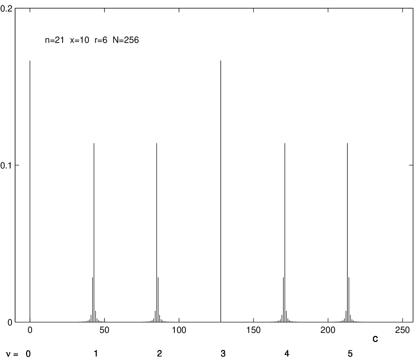
Probability distribution P​(c)𝑃𝑐P(c) of the Quantum Computer output
state number c𝑐c. The integer to factorize n=21𝑛21n=21 and the auxiliary
integer x=10π‘₯10x=10. The order of x​(mod​n)π‘₯mod𝑛x\ ({{\rm mod}\ n}) is r=6π‘Ÿ6r=6. The size of the
computer is qA=8subscriptπ‘žπ΄8q_{A}=8 qubits corresponding to N=256𝑁256N=256.

The probability that the quantum computer ends in state |c>ket𝑐|c\!\!> is

P​(c)=1N2β€‹βˆ‘k=0rβˆ’1sin2⁑[π​(M+1)​r​c/N]sin2⁑[π​r​c/N]P𝑐1superscript𝑁2superscriptsubscriptπ‘˜0π‘Ÿ1superscript2πœ‹π‘€1π‘Ÿπ‘π‘superscript2πœ‹π‘Ÿπ‘π‘{\rm P}(c)=\frac{1}{N^{2}}\sum_{k=0}^{r-1}\frac{\sin^{2}[\pi(M+1)rc/N]}{\sin^{2}[\pi rc/N]} (8)

The parameter M=⌊(Nβˆ’kβˆ’1)/rβŒ‹π‘€π‘π‘˜1π‘ŸM=\lfloor(N-k-1)/r\rfloor. Let k0subscriptπ‘˜0k_{0} be the smallest integer such that

⌊(Nβˆ’k0βˆ’1)/rβŒ‹=⌊(Nβˆ’r)/rβŒ‹=M0𝑁subscriptπ‘˜01π‘Ÿπ‘π‘Ÿπ‘Ÿsubscript𝑀0\lfloor(N-k_{0}-1)/r\rfloor=\lfloor(N-r)/r\rfloor=M_{0}

Then

P​(c)=k0N2​sin2⁑[π​(M0+1)​r​c/N]sin2⁑[π​r​c/N]+rβˆ’k0N2​sin2⁑[π​M0​r​c/N]sin2⁑[π​r​c/N]P𝑐subscriptπ‘˜0superscript𝑁2superscript2πœ‹subscript𝑀01π‘Ÿπ‘π‘superscript2πœ‹π‘Ÿπ‘π‘π‘Ÿsubscriptπ‘˜0superscript𝑁2superscript2πœ‹subscript𝑀0π‘Ÿπ‘π‘superscript2πœ‹π‘Ÿπ‘π‘{\rm P}(c)=\frac{k_{0}}{N^{2}}\ \frac{\sin^{2}[\pi(M_{0}+1)rc/N]}{\sin^{2}[\pi rc/N]}+\frac{r-k_{0}}{N^{2}}\ \frac{\sin^{2}[\pi M_{0}rc/N]}{\sin^{2}[\pi rc/N]} (9)

P​(c)𝑃𝑐P(c) is illustrated for n=21=3β‹…7𝑛21β‹…37n=21=3\cdot 7 and x=10π‘₯10x=10 in Fig. 1. The QC register size qA=⌈log2⁑nβŒ‰=9subscriptπ‘žπ΄subscript2𝑛9q_{A}=\lceil\log_{2}n\rceil=9 making N=256𝑁256N=256

The function (9) with c𝑐c replaced by a real continuous variable ΟƒπœŽ\sigma is the envelope of the discrete probability distribution. It is periodic and has peaks at

σν=Ξ½r​N;Ξ½=0,1,…​rβˆ’1formulae-sequencesubscriptπœŽπœˆπœˆπ‘Ÿπ‘πœˆ01β€¦π‘Ÿ1\sigma_{\nu}=\frac{\nu}{r}N;\ \ \ \nu=0,1,\ldots r-1 (10)

Let cΞ½subscriptπ‘πœˆc_{\nu} denote the integer part of σνsubscript𝜎𝜈\sigma_{\nu}

cΞ½=βŒŠΟƒΞ½βŒ‹=ΟƒΞ½βˆ’Ξ΄Ξ½;;0≀δν<1c_{\nu}=\lfloor\sigma_{\nu}\rfloor=\sigma_{\nu}-\delta_{\nu};\ \ \ ;0\leq\delta_{\nu}<1 (11)

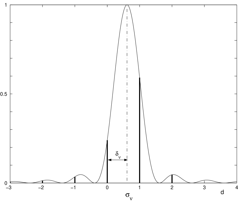
The parameters are illustrated in Fig. 2.
Refer to caption
Figure 2:

The shape of the peaks of the probability distribution P​(c)𝑃𝑐P(c).

The output c=cΞ½+d𝑐subscriptπ‘πœˆπ‘‘c=c_{\nu}+d from the quantum computer is characterized by two random variables, the displacement parameter δνsubscriptπ›Ώπœˆ\delta_{\nu}, and the integer valued parameter d=cβˆ’cν𝑑𝑐subscriptπ‘πœˆd=c-c_{\nu} representing the deviation within the peak.

3 Post quantum calculations

The ratio r/Ξ½π‘Ÿπœˆr/\nu is estimated as the largest convergent with nominator less than n𝑛n in a continued fractions expansion of N/c𝑁𝑐N/c. This procedure generates the fraction r/Ξ½π‘Ÿπœˆr/\nu closest to N/c𝑁𝑐N/c, see e.g. [3], Theorem 181.

The algorithm is based on the relation

xrβˆ’1=(xr/2+1)​(xr/2βˆ’1)≑0​(mod​n)superscriptπ‘₯π‘Ÿ1superscriptπ‘₯π‘Ÿ21superscriptπ‘₯π‘Ÿ210mod𝑛x^{r}-1=(x^{r/2}+1)(x^{r/2}-1)\equiv 0\ ({\rm mod}\ n) (12)

which shows (means?) that the factors p1subscript𝑝1p_{1} and p2subscript𝑝2p_{2} are possible divisors of (xr/2Β±1)plus-or-minussuperscriptπ‘₯π‘Ÿ21(x^{r/2}\pm 1).

To obtain a correct value of r/Ξ½π‘Ÿπœˆr/\nu the ratio c/N𝑐𝑁c/N must not be too far from Ξ½/rπœˆπ‘Ÿ\nu/r The incorrect value closest the correct Ξ½/rπœˆπ‘Ÿ\nu/r is (Ξ½+1)/(r+1)𝜈1π‘Ÿ1(\nu+1)/(r+1). The difference

Ξ”=Ξ½+1r+1βˆ’Ξ½r=rβˆ’Ξ½r​(r+1)Ξ”πœˆ1π‘Ÿ1πœˆπ‘Ÿπ‘Ÿπœˆπ‘Ÿπ‘Ÿ1\Delta=\frac{\nu+1}{r+1}-\frac{\nu}{r}=\frac{r-\nu}{r(r+1)} (13)

takes its lowest value Ξ”=1/r​(r+1)Ξ”1π‘Ÿπ‘Ÿ1\Delta=1/r(r+1) for Ξ½=rβˆ’1πœˆπ‘Ÿ1\nu=r-1. The maximal value of rπ‘Ÿr is less than nβˆ’1𝑛1n-1 and Ξ”m​i​n>1/(nβˆ’1)​nsubscriptΞ”π‘šπ‘–π‘›1𝑛1𝑛\Delta_{min}>1/(n-1)n The difference between the correct Ξ½/rπœˆπ‘Ÿ\nu/r and c/N𝑐𝑁c/N is

Ξ”c​(d)=|cNβˆ’Ξ½r|=|dβˆ’Ξ΄Ξ½N|subscriptΞ”π‘π‘‘π‘π‘πœˆπ‘Ÿπ‘‘subscriptπ›Ώπœˆπ‘\Delta_{c}(d)=\Big{|}\frac{c}{N}-\frac{\nu}{r}\Big{|}=\Big{|}\frac{d-\delta_{\nu}}{N}\Big{|} (14)

For Nβ‰₯n2𝑁superscript𝑛2N\geq n^{2} the distances Ξ”c​(0)subscriptΔ𝑐0\Delta_{c}(0) and Ξ”c​(1)subscriptΔ𝑐1\Delta_{c}(1) are both less than Ξ”m​i​nsubscriptΞ”π‘šπ‘–π‘›\Delta_{min} and the continued fractions expansion always produces the correct order rπ‘Ÿr, when d=0𝑑0d=0 or d=1𝑑1d=1.

Substitution of c=ν​N/r+dβˆ’Ξ΄Ξ½π‘πœˆπ‘π‘Ÿπ‘‘subscriptπ›Ώπœˆc=\nu N/r+d-\delta_{\nu} into (8) yields

P​(c)=1N2β€‹βˆ‘k=0rβˆ’1sin2⁑[π​(M+1)​ν+π​(M+1)​r​(dβˆ’Ξ΄Ξ½)/N]sin2⁑[π​ν+π​r​(dβˆ’Ξ΄Ξ½)/N]P𝑐1superscript𝑁2superscriptsubscriptπ‘˜0π‘Ÿ1superscript2πœ‹π‘€1πœˆπœ‹π‘€1π‘Ÿπ‘‘subscriptπ›Ώπœˆπ‘superscript2πœ‹πœˆπœ‹π‘Ÿπ‘‘subscriptπ›Ώπœˆπ‘{\rm P}(c)=\frac{1}{N^{2}}\sum_{k=0}^{r-1}\frac{\sin^{2}[\pi(M+1)\nu+\pi(M+1)r(d-\delta_{\nu})/N]}{\sin^{2}[\pi\nu+\pi r(d-\delta_{\nu})/N]} (15)

The factor (M+1)​r/N=1βˆ’Ο΅π‘€1π‘Ÿπ‘1italic-Ο΅(M+1)r/N=1-\epsilon with Ο΅<r/N<1/nitalic-Ο΅π‘Ÿπ‘1𝑛\epsilon<r/N<1/n and since r/N is small

P​(d)=sin2⁑(π​δν)Ο€2​(dβˆ’Ξ΄Ξ½)2P𝑑superscript2πœ‹subscriptπ›Ώπœˆsuperscriptπœ‹2superscript𝑑subscriptπ›Ώπœˆ2{\rm P}(d)=\frac{\sin^{2}(\pi\delta_{\nu})}{{\pi}^{2}(d-\delta_{\nu})^{2}} (16)

is an accurate approximation. The probability, averaged over δνsubscriptπ›Ώπœˆ\delta_{\nu}, that d=0𝑑0d=0 or d=1𝑑1d=1 is equal to 0.902.

For more common values of rπ‘Ÿr and ν𝜈\nu the probability of an incorrect result is much smaller and the continued fractions procedure can safely be assumed to produce a ratio Ξ½/rπœˆπ‘Ÿ\nu/r with rπ‘Ÿr is the correct order of x​(mod​n)π‘₯mod𝑛x\ ({\rm mod}\ n) and ν𝜈\nu an unknown random number Ξ½=1,2,…​rβˆ’1𝜈12β€¦π‘Ÿ1\nu=1,2,\ldots r-1. Trying neighboring states, as has been suggested in the literature, i.e [2] p 320, will have no effect.

The relation (12) requires rπ‘Ÿr to be even and since all even values of ν𝜈\nu will have at least a factor 2 in common with rπ‘Ÿr the probability that rπ‘Ÿr and ν𝜈\nu are relatively prime and the correct order rπ‘Ÿr is obtained directly is less than 0.5.

The algorithm fails when Ξ½=0𝜈0\nu=0, the probability for this is equal to 1/r1π‘Ÿ1/r and can usually be neglected.

4 Generation of the integer xπ‘₯x

The properties of xπ‘₯x is of fundamental importance for the function of the prime factorization algorithm. As shown below, for a random xπ‘₯x and n𝑛n the probability that the factorization procedure fails is 1/3.

Consider two prime numbers p1subscript𝑝1p_{1} and p2subscript𝑝2p_{2} together with an arbitrary integer xπ‘₯x. Let r1subscriptπ‘Ÿ1r_{1} and r2subscriptπ‘Ÿ2r_{2} denote the order of xπ‘₯x mod p1subscript𝑝1p_{1} and mod p2subscript𝑝2p_{2} respectively. The order rπ‘Ÿr of n=p1​p2𝑛subscript𝑝1subscript𝑝2n=p_{1}p_{2} is equal to lcm​(r1​r2)lcmsubscriptπ‘Ÿ1subscriptπ‘Ÿ2{\rm lcm}(r_{1}r_{2}), the least common multiplier of r1subscriptπ‘Ÿ1r_{1} and r2subscriptπ‘Ÿ2r_{2}. The factorization procedure fails when rπ‘Ÿr is odd i.e when both r1subscriptπ‘Ÿ1r_{1} and r2subscriptπ‘Ÿ2r_{2} are odd. With the assumption that a random xπ‘₯x generates random and independent values of r1subscriptπ‘Ÿ1r_{1} and r2subscriptπ‘Ÿ2r_{2} and the probability of both being odd is P​(A)=1/4𝑃𝐴14P(A)=1/4.

The only other case when the procedure fails is when

xr/2β‰‘βˆ’1​(mod​n)superscriptπ‘₯π‘Ÿ21mod𝑛x^{r/2}\equiv-1\ ({\rm mod}\ n) (17)

in which case gcd​(xr/2βˆ’1)=1gcdsuperscriptπ‘₯π‘Ÿ211{\rm gcd}(x^{r/2}-1)=1 and gcd​(xr/2+1)=ngcdsuperscriptπ‘₯π‘Ÿ21𝑛{\rm gcd}(x^{r/2}+1)=n.

The relation (17) is satisfied only if both r1subscriptπ‘Ÿ1r_{1} and r2subscriptπ‘Ÿ2r_{2} are even and containing identical factors 2ksuperscript2π‘˜2^{k} which for random r1subscriptπ‘Ÿ1r_{1} and r2subscriptπ‘Ÿ2r_{2} occurs with probability

P​(B)=14β€‹βˆ‘k=1∞122​k=112𝑃𝐡14superscriptsubscriptπ‘˜11superscript22π‘˜112P(B)=\frac{1}{4}\sum_{k=1}^{\infty}\frac{1}{2^{2k}}=\frac{1}{12} (18)

making the total probability of failure P​(A)+P​(B)=13𝑃𝐴𝑃𝐡13P(A)+P(B)=\frac{1}{3}

Ekert and Jozsa [4] assume n𝑛n fixed but arbitrary and showed that

P​r​[r​odd​o​r​xr/2β‰‘βˆ’1​(mod​n)]≀1/2π‘ƒπ‘Ÿdelimited-[]π‘Ÿoddπ‘œπ‘Ÿsuperscriptπ‘₯π‘Ÿ21mod𝑛12Pr[r\ {\rm odd}\ or\ x^{r/2}\equiv-1\ ({\rm mod}\ n)]\leq 1/2

If xπ‘₯x contains any of the prime factors of n𝑛n the equation xr≑1​(mod​n)superscriptπ‘₯π‘Ÿ1mod𝑛x^{r}\equiv 1\ ({{\rm mod}\ n}) has no solution and the algorithm fails. The probability for this is extremely small for any sizable values of n𝑛n. It is easy to test gcd​(x,n)gcdπ‘₯𝑛{\rm gcd}(x,n) before using xπ‘₯x and if there is a common factor no QC calculation is needed.

5 Conclusions

For a quantum computer of size qA=2​msubscriptπ‘žπ΄2π‘šq_{A}=2m factorizing an mπ‘šm bit number the output from the post quantum calculations is the correct order rπ‘Ÿr or ro​u​t=r/ΞΌsubscriptπ‘Ÿπ‘œπ‘’π‘‘π‘Ÿπœ‡r_{out}=r/\mu with ΞΌπœ‡\mu a factor common to rπ‘Ÿr and ν𝜈\nu. It is easy to check if xro​u​t≑1​(mod​n)superscriptπ‘₯subscriptπ‘Ÿπ‘œπ‘’π‘‘1mod𝑛x^{r_{out}}\equiv 1\ ({\rm mod}\ n) and if not the unknown ΞΌπœ‡\mu may be found by trial or possibly by a more a efficient algorithm. From simulation results 111Quantum Computer simulation programs are available at
http//www.s3.kth.se/∼similar-to\simeinarson/
it has been observed that one of the prime factors can sometimes be obtained by the gcd algorithm from r/ΞΌπ‘Ÿπœ‡r/\mu.An alternative is to rerun the QC with the same xπ‘₯xto generate a new output c𝑐c.

If the final value of rπ‘Ÿr is either odd or satisfies (17) the algorithm fails and the QC has to be run with a new xπ‘₯x, which means that the quantum circuitry needs to be modified.

Acknowledgment

Thanks are due to Johan HΓ₯stad for helpful discussions.

References

  • [1] Michael A. Nielsen and Isaac L. Chuang
    Quantum Computation and Quantum Information
    Cambridge University Press, Cambridge, 2000.
  • [2] Peter W. Shor
    β€œPolynomial-Time Algorithms for Prime Factorization and Discrete Logarithms on a Quantum Computer”
    SIAM Review vol 41, No. 2, pp 301-332.
  • [3] G. H. Hardy and E. M. Wright
    An Introduction to the Theory of Numbers
    Oxford University Press, Oxford, 1979.
  • [4] Artur Ekert and Richard Jozsa
    β€œQuantum computation and Shor’s factoring algorithm”
    Reviews of Modern Physics vol 68, No. 3, pp 733-753.