Optomechanical detection of weak forces
Abstract
Optomechanical systems are often used for the measurement of weak forces. Feedback loops can be used in these systems for achieving noise reduction. Here we show that even though feedback is not able to improve the signal to noise ratio of the device in stationary conditions, it is possible to design a nonstationary strategy able to improve the sensitivity.
keywords:
Optomechanical devices, feedback, high-sensitive detection1 INTRODUCTION
Optomechanical devices are used in high sensitivity measurements, as the interferometric detection of gravitational waves [1], and in atomic force microscopes [2]. Up to now, the major limitation to the implementation of sensitive optical measurements is given by thermal noise [3]. Some years ago it has been proposed [4] to reduce thermal noise by means of a feedback loop based on homodyning the light reflected by the oscillator, playing the role of a cavity mirror. This proposal has been then experimentally realized [5, 6, 7] using the “cold damping” technique [8], which is physically analogous to that proposed in Ref. [4] and which amounts to applying a viscous feedback force to the oscillating mirror. In these experiments, the viscous force is provided by the radiation pressure of another laser beam, intensity-modulated by the time derivative of the homodyne signal.
Both the scheme of Ref. [4] and the cold damping scheme of Refs. [5, 6, 7] cool the mirror by overdamping it, thereby strongly decreasing its mechanical susceptibility at resonance. As a consequence, the oscillator does not resonantly respond to the thermal noise, yielding in this way an almost complete suppression of the resonance peak in the noise power spectrum, which is equivalent to cooling. However, the two feedback schemes cannot be directly applied to improve the detection of weak forces. In fact the strong reduction of the mechanical susceptibility at resonance means that the mirror does not respond not only to the noise but also to the signal. This means that the signal to noise ratio (SNR) of the device in stationary conditions is actually never improved [9, 10]. Despite that, here we show how it is possible to design a nonstationary strategy able to significantly increase the SNR for the detection of impulsive classical forces acting on the oscillator. This may be useful for microelectromechanical systems, where the search for quantum effects in mechanical systems is very active [11], as well as for the detection of gravitational waves [1].
2 The model
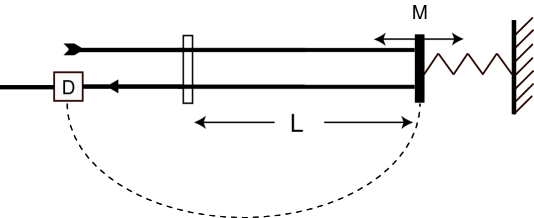
We shall consider a simple example of optomechanical system, a Fabry-Perot cavity with a movable end mirror (see Fig. 1 for a schematic description). The optomechanical coupling between the mirror and the cavity field is realized by the radiation pressure. The electromagnetic field exerts a force which is proportional to the intensity of the field, which, at the same time, is phase-shifted by an amount proportional to the mirror displacement from its equilibrium position. The mirror motion is the result of the excitation of many vibrational modes, including internal acoustic modes. However here we shall study the spectral detection of weak forces acting on the mirror and in this case one can focus on a single mechanical mode only, by considering a detection bandwidth including a single mechanical resonance peak [12]. Optomechanical devices are able to reach the sensitivity limits imposed by quantum mechanics [10] and therefore we describe the mechanical mode as a single quantum harmonic oscillator with mass and frequency .
 |
When is much smaller than the cavity free spectral range, one can focus on one cavity mode only, because photon scattering into other modes can be neglected [13]. Moreover, in this regime, the generation of photons due to the Casimir effect, and also retardation and Doppler effects are completely negligible [14]. The system is then described by the following two-mode Hamiltonian [14]
| (1) |
where is the cavity mode annihilation operator with optical frequency , is the classical force to be detected, and describes the coherent input field with frequency driving the cavity. The quantity is related to the input laser power by , being the photon decay rate. Moreover, and are the dimensionless position and momentum operator of the movable mirror. It is , and represents the optomechanical coupling constant, with the equilibrium cavity length.
The dynamics of an optomechanical system is also influenced by the dissipative interaction with external degrees of freedom. The cavity mode is damped due to the photon leakage through the mirrors which couple the cavity mode with the continuum of the outside electromagnetic modes. For simplicity we assume that the movable mirror has perfect reflectivity and that transmission takes place through the fixed mirror only. The mechanical mode undergoes Brownian motion caused by the uncontrolled coupling with other internal and external modes at thermal equilibrium. We shall neglect in our treatment all the technical noise sources: we assume that the driving laser is stabilized in intensity and frequency and we neglect the electronic noise in the detection circuit. Including these supplementary noise sources is however quite straightforward (see for example [15]). Moreover recent experiments have shown that classical laser noise can be made negligible in the relevant frequency range [3, 16].
The dynamics of the system can be described by the following set of coupled quantum Langevin equations (QLE) (in the interaction picture with respect to )
| (2) | |||||
| (3) | |||||
| (4) |
where is the input noise operator [17] associated with the vacuum fluctuations of the continuum of modes outside the cavity, having the following correlation functions
| (5) | |||
| (6) |
Furthermore, is the quantum Langevin force acting on the mirror, with the following correlation function [18],
| (7) |
with the bath temperature, the mechanical decay rate, the Boltzmann constant, and the frequency cutoff of the reservoir spectrum.
In standard applications the driving field is very intense so that the system is characterized by a semiclassical steady state with the internal cavity mode in a coherent state , and a new equilibrium position for the mirror, displaced by with respect to that with no driving field. The steady state amplitude is given by the solution of the classical nonlinear equation . In this case, the dynamics is well described by linearizing the QLE (2)-(4) around the steady state. Redefining with and the quantum fluctuations around the classical steady state, introducing the field phase and field amplitude , and choosing the resulting cavity mode detuning (by properly tuning the driving field frequency ), the linearized QLEs can be rewritten as
| (8) | |||||
| (9) | |||||
| (10) | |||||
| (11) |
where we have introduced the phase input noise and the amplitude input noise .
3 Position measurement and feedback
As it is shown by Eq. (10), when the driving and the cavity fields are resonant, the dynamics is simpler because only the phase quadrature is affected by the mirror position fluctuations , while the amplitude quadrature is not. Therefore the mechanical motion of the mirror can be detected by monitoring the phase quadrature . The mirror position measurement is commonly performed in the large cavity bandwidth limit , , when the cavity mode dynamics adiabatically follows that of the movable mirror and it can be eliminated, that is, from Eq. (10),
| (12) |
and from Eq. (11). The experimentally detected quantity is the output homodyne photocurrent [19, 20, 21]
| (13) |
where is the detection efficiency and is a generalized phase input noise, coinciding with the input noise in the case of perfect detection , and taking into account the additional noise due to the inefficient detection in the general case [20]. This generalized phase input noise can be written in terms of a generalized input noise as . The quantum noise is correlated with the input noise and it is characterized by the following correlation functions [20]
| (14) | |||
| (15) | |||
| (16) |
The output of the homodyne measurement may be used to devise a phase-sensitive feedback loop to control the dynamics of the mirror, as in the original proposal[4], or in cold damping schemes[5, 6, 7, 8]. Let us now see how these two feedback schemes modify the quantum dynamics of the mirror.
In the scheme of Ref.[4], the feedback loop induces a continuous position shift controlled by the output homodyne photocurrent . This effect of feedback manifests itself in an additional term in the QLE for a generic operator given by
| (17) |
where is the feedback transfer function, and is a feedback gain factor. The implementation of this scheme is nontrivial because it is equivalent to add a feedback interaction linear in the mirror momentum, as it could be obtained with a charged mirror in a homogeneous magnetic field. For this reason here we shall refer to it as “momentum feedback” (see, however, the recent parametric cooling scheme demonstrated in Ref. [7], showing some similarity with the feedback scheme of Ref. [4]).
Feedback is characterized by a delay time which is essentially determined by the electronics and is always much smaller than the typical timescale of the mirror dynamics. It is therefore common to consider the zero delay-time limit . For linearized systems, the limit can be taken directly in Eq. (17) [10], so to get the following QLE in the presence of feedback
| (18) | |||||
| (19) | |||||
| (20) | |||||
| (21) |
where we have used Eq. (13). After the adiabatic elimination of the radiation mode (see Eq. (12)), and introducing the rescaled, dimensionless, input power of the driving laser , and the rescaled feedback gain , the above equations reduce to
| (22) | |||||
| (23) |
This treatment explicitly includes the limitations due to the quantum efficiency of the detection, but neglects other possible technical imperfections of the feedback loop, as for example the electronic noise of the feedback loop, whose effects have been discussed in [6].
Cold damping techniques have been applied in classical electromechanical systems for many years [8], and only recently they have been proposed to improve cooling and sensitivity at the quantum level [22]. This technique is based on the application of a negative derivative feedback, which increases the damping of the system without correspondingly increasing the thermal noise [22]. This technique has been succesfully applied to an optomechanical system composed of a high-finesse cavity with a movable mirror in [5, 6, 7]. In these experiments, the displacement of the mirror is measured with very high sensitivity [3, 7], and the obtained information is fed back to the mirror via the radiation pressure of another, intensity-modulated, laser beam, incident on the back of the mirror. Cold damping is obtained by modulating with the time derivative of the homodyne signal, in such a way that the radiation pressure force is proportional to the mirror velocity. A quantum description of cold damping can be obtained using either quantum network theory [22], or a quantum Langevin description [9, 10]. In this latter treatment, cold damping implies the following additional term in the QLE for a generic operator ,
| (24) |
where and are the corresponding transfer function and gain factor. As in the previous case, one usually assume a Markovian feedback loop with negligible delay. Since one needs a derivative feedback, this would ideally imply , i.e., , , even though, in practice, it is sufficient to satisfy this condition within the detection bandwidth. In this case, the QLEs for the cold damping feedback scheme become
| (25) | |||||
| (26) | |||||
| (27) | |||||
| (28) |
Adiabatically eliminating the cavity mode, and introducing the rescaled, dimensionless feedback gain , one has
The presence of an ideal derivative feedback implies the introduction of two new quantum input noises, and , whose correlation functions can be simply obtained by differentiating the corresponding correlation functions of and [10]. However, as discussed above, these “differentiated” correlation functions have to be considered as approximate expressions valid within the detection bandwidth only.
The two sets of QLE for the mirror Heisenberg operators show that the two feedback schemes are not exactly equivalent. They are however physically analogous, as it can be seen, for example, by looking at the Fourier transforms of the corresponding mechanical susceptibilities [9, 10]
| (29) |
for the momentum feedback scheme, and
| (30) |
for cold damping. These expressions show that in both schemes the main effect of feedback is the modification of mechanical damping (). Therefore, also momentum feedback provides a cold damping effect of increased damping without an increased temperature. In this latter case, one has also a frequency renormalization , which is however negligible when the mechanical quality factor is large.
4 Spectral measurements and their sensitivity
Spectral measurements are performed whenever the classical force to detect has a characteristic frequency. We adopt a very general treatment which can be applied even in the case of nonstationary measurements. The explicitly measured quantity is the output homodyne photocurrent , and therefore we define the signal as
| (31) |
where is a “filter” function, approximately equal to one in the time interval in which the measurement is performed, and equal to zero otherwise. The spectral measurement is stationary when is very large, i.e. is much larger than all the typical timescales of the system. Using Eq. (12) and the input-output relation (13), the signal can be rewritten as
| (32) |
where and are the Fourier transforms of the force and of the filter function, respectively, and is equal to or , according to the feedback scheme considered.
The noise corresponding to the signal is given by its “variance”; since the signal is zero when , the noise spectrum can be generally written as
| (33) |
where the subscript means evaluation in the absence of the external force. Using again (12), Eqs. (13), and the input noises correlation functions (5)-(6) and (14)-(16), the spectral noise can be rewritten as
| (34) |
where is the symmetrized correlation function of the oscillator position. This very general expression of the noise spectrum is nonstationary because it depends upon the nonstationary correlation function . The last term in Eq. (34) is the shot noise term due to the radiation input noise.
4.1 Stationary spectral measurements
Spectral measurements are usually performed in the stationary case, that is, using a measurement time much larger than the typical oscillator timescales. The most significant timescale is the mechanical relaxation time, which is in the absence of feedback and () in the presence of feedback. In the stationary case, the oscillator is relaxed to equilibrium and, redefining , the correlation function in Eq. (34) is replaced by the stationary correlation function . Moreover, for very large , one has and, defining the measurement time so that , Eq. (34) assumes the form
| (35) |
where
| (36) |
is the stationary position noise spectrum. This noise spectrum can be evaluated by solving the quantum Langevin equations in the presence of the two feedback schemes and Fourier transforming [10]. One obtains
| (37) |
for the momentum feedback scheme and
| (38) |
for the cold damping scheme, where (i=mf,cd) are the Fourier transforms of the feedback transfer functions and is a gate function equal to within the frequency interval and zero outside. The position noise spectrum for the momentum feedback essentially coincides with that already obtained in [4], except that in that paper the high-temperature (), Markovian feedback (), and infinite cutoff () approximations have been considered. The noise spectrum in the cold damping case of Eq. (38) instead essentially reproduces the one obtained in [23], with the difference that in Ref. [23] the homodyne detection efficiency is set equal to one, and the Markovian feedback (), and infinite cutoff () approximations have been again considered. The comparison between Eqs. (38) and (37) shows once again the similarities of the two schemes. The only differences lie in the different susceptibilities and in the feedback-induced noise term, which has an additional factor in the momentum feedback case, which is however usually negligible with good mechanical quality factors. In fact, the two noise spectra are practically indistinguishable in a very large parameter region.
The effectively detected position noise spectrum is not given by Eqs. (38) and (37), but it is the noise spectrum associated to the output homodyne photocurrent of Eq. (35) rescaled to a position spectrum. This homodyne-detected position noise spectrum is actually subject also to cavity filtering, yielding an experimental high frequency cutoff , which however does not appear in our expressions because we have adiabatically eliminated the cavity mode from the beginning. Therefore the noise spectrum derived here is correct only for . However, this is not a problem because the frequencies of interest (i.e. those within the detection bandwidth) are always much smaller than , and also than . Within the detection bandwidth one can safely approximate , and in Eqs. (38) and (37). Therefore, using Eq. (35), the detected position noise spectrum can be written
| (39) |
where refers to the momentum feedback case and to the cold damping case.
This spectrum has four contributions: the radiation pressure noise term, proportional to the input power , the feedback-induced term proportional to the squared gain and inversely proportional to , the Brownian motion term which is independent of , and the shot noise term inversely proportional to . The main effect of feedback on the noise spectrum is the modification of the susceptibility due to the increase of damping, yielding the suppression and widening of the resonance peak. This peak suppression in the noise spectrum has been already predicted and illustrated in [4, 23], and experimentally verified for the cold damping case in [5, 6]. It has been shown [23, 10] that both feedback schemes are able to arbitrarily reduce the displacement noise at resonance. This noise reduction at resonance is similar to that occurring to an oscillator with increasing damping, except that in the present case, also the feedback-induced noise increases with the gain, and it can be kept small only if the input power is correspondingly increased in order to maintain the optimal value minimizing the noise [10]. This arbitrary reduction of the position noise in a given frequency bandwidth with increasing feedback gain does not hold if the input power is kept fixed. In this latter case, the noise has a frequency-dependent lower bound which cannot be overcome by increasing the gain.
In the case of stationary spectral measurements also the expression of the signal simplifies. In fact, one has , and Eq. (32) becomes . The stationary SNR, , is now simply obtained dividing this signal by the noise of Eq. (35),
| (40) |
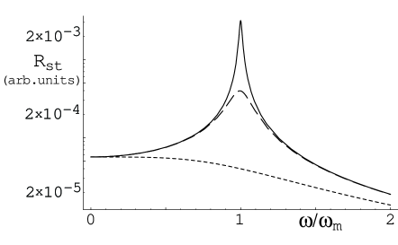
where again refers to the momentum feedback case and to the cold damping case. It is easy to see that, in both cases, feedback always lowers the stationary SNR at any frequency, (except at , where the SNR for the cold damping case does not depend upon the feedback gain). This is shown in Fig. 2, where the stationary SNR in the case of an ideal impulsive force (that is, is a constant) is plotted for three values of the feedback gain. The curves refer to both feedback schemes because the two cases gives always practically indistinguishable results, except for very low values of . This result can be easily explained. In fact, the main effect of feedback is to decrease the mechanical susceptibility at resonance (see Eqs. (29) and (30)), so that the oscillator is less sensitive not only to the noise but also to the signal. Therefore, even though the two feedback schemes are able to provide efficient cooling and noise reduction in narrow bandwidths for the mechanical mode, they cannot be used to improve the sensitivity of the optomechanical device for stationary measurements. In the next section we shall see how cooling via feedback can be used to improve the sensitivity for the detection of impulsive forces, using an appropriate nonstationary strategy.
 |
5 High-sensitive nonstationary measurements
The two feedback schemes discussed here achieve noise reduction through a modification of the mechanical susceptibility. However, this modification does not translate into a sensitivity improvement because at the same time it strongly degrades the detection of the signal. The sensitivity of position measurements would be improved if the oscillator mode could keep its intrinsic susceptibility, unmodified by feedback, together with the reduced noise achieved by the feedback loop. This is obviously impossible in stationary conditions, but a situation very similar to this ideal one can be realized in the case of the detection of an impulsive force, that is, with a time duration much shorter than the mechanical relaxation time (in the absence of feedback), . In fact, one could use the following nonstationary strategy: prepare at the mirror mode in the stationary state cooled by feedback, then suddenly turn off the feedback loop and perform the spectral measurement in the presence of the impulsive force for a time , such that . In such a way, the force spectrum is still well reproduced, and the mechanical susceptibility is the one without feedback (even though modified by the short measurement time ). At the same time, the mechanical mode is far from equilibrium during the whole measurement, and its noise spectrum is different from the stationary form of Eq. (39), being mostly determined by the cooled initial state. As long as , heating, that is, the approach to the hotter equilibrium without feedback, will not affect and increase too much the noise spectrum. Therefore, one expects that as long as the measurement time is sufficiently short, the SNR for the detection of the impulsive force (which has now to be evaluated using the most general expressions (32) and (34)) can be significantly increased by this nonstationary strategy.
It is instructive to evaluate explicitely the nonstationary noise spectrum of Eq. (34) for the above measurement strategy. Simple analytical results are obtained by choosing the following filter function ( is the Heavyside step function), satisfying . Let us consider the cold damping case first. Solving the QLE of the system by taking the equilibrium state in the presence of feedback as initial condition, one arrives at the following expression for the detected nonstationary noise spectrum [10]
| (41) |
where is the Fourier transform of the susceptibility in the absence of feedback (see Eq. (29) with or Eq. (30) with ) and we have used the high temperature approximation for the Brownian noise. Moreover, and are the stationary variances in the presence of feedback,
| (42) | |||
| (43) |
where is given by Eq. (38). The nonstationary noise spectrum for the momentum feedback case is analogous to that of Eq. (41), except that one has to use the corresponding stationary values as initial conditions (there is an additional term due to the fact that for momentum feedback [10]). However, as for the stationary case, one can check that the two feedback schemes give indistinguishable results in a large parameter region. Therefore we shall discuss the cold damping case only from now on, even though the same results also apply to the momentum feedback case with the replacement .
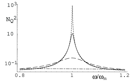
It is easy to check from Eq. (41) that the stationary noise spectrum corresponding to the situation with no feedback is recovered in the limit of large , as expected, when the terms inversely proportional to and depending on the initial conditions become negligible, and . In the opposite limit of small instead, the terms associated to the cooled, initial conditions are dominant, and since the stationary terms are still small, this means having a reduced, nonstationary noise spectrum. This is clearly visible in Fig. 3, where the nonstationary noise spectrum is plotted for different values of the measurement time , (dotted line), (full line), (dashed line), (dot-dashed line). The resonance peak is significantly suppressed for decreasing , even if it is simultaneously widened, so that one can even have a slight increase of noise out of resonance.
 |
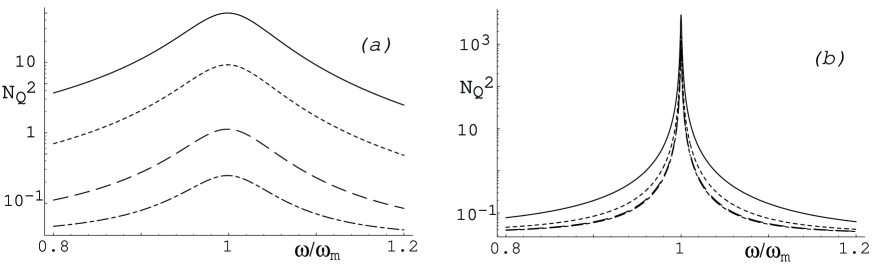
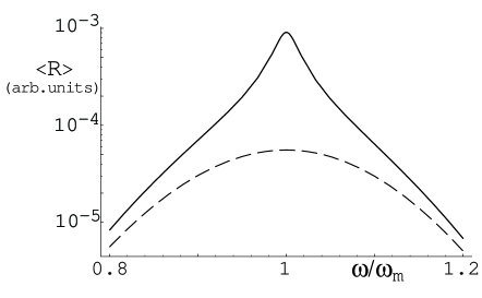
The effect of the terms depending upon the feedback-cooled initial conditions on the nonstationary noise is shown in Fig. 4, where the noise spectrum is plotted for different values of the feedback gain at a fixed value of . In Fig. 4a, is plotted at for (full line), (dotted line), (dashed), (dot-dashed). For this low value of , the noise terms depending on the initial conditions are dominant, and increasing the feedback gain implies reducing the initial variances, and therefore an approximately uniform noise suppression at all frequencies. In Fig. 4b, is instead plotted at for (full line), (dotted line), (dashed), (dot-dashed). In this case, the feedback-gain-independent, stationary terms become important, and the effect of feedback on the noise spectrum becomes negligible.
 |
The significant noise reduction attainable at short measurement times is not only due to the feedback-cooled initial conditions, but it is also caused by the effective reduction of the mechanical susceptibility given by the short measurement time, . This lowered susceptibility yields a simultaneous reduction of the signal at small measurement times , and therefore the behavior of the nonstationary SNR may be nontrivial. However, one expects that impulsive forces at least can be satisfactorily detected using a short measurement time, because the noise can be kept very small and the corresponding sensitivity increased. Let us check this fact considering the case of the impulsive force
| (44) |
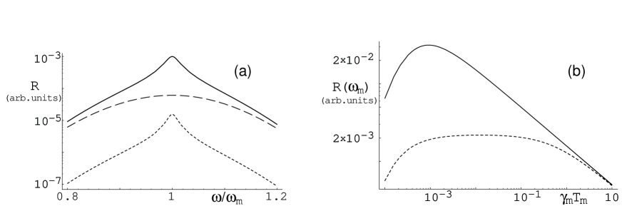
where is the force duration, its “arrival time”, and its carrier frequency. The corresponding SNR is obtained dividing the signal of Eq. (31) by the nonstationary noise spectra of Eq. (41), and it is shown in Fig. 5. As anticipated, the sensitivity of the optomechanical device is improved using feedback in a nonstationary way. In Fig. 5a, the spectral SNR, , is plotted for different values of feedback gain and measurement time. The full line refers to and , the dashed line to the situation with no feedback and the same measurement time, and ; finally the dotted line refers to a “standard” measurement, that is, no feedback and a stationary measurement, with a long measurement time, . The proposed nonstationary measurement scheme, “cool and measure”, gives the highest sensitivity. This is confirmed also by Fig. 5b, where the SNR at resonance, , when feedback cooling is used with (full line), and without feedback cooling (dotted line), is plotted as a function of the rescaled measurement time . The preparation of the mirror in the cooled initial state yields a better sensitivity for any measurement time. As expected, the SNR in the presence of feedback approaches that without feedback in the stationary limit , when the effect of the initial cooling becomes irrelevant. Fig. 5 refer to a resonant () impulsive force with and , while the other parameters are , , , .
 |
The proposed nonstationary strategy can be straightforwardly applied whenever the “arrival time” of the impulsive force is known: feedback has to be turned off just before the arrival of the force. However, the scheme can be easily adapted also to the case of an impulsive force with an unknown arrival time, as for example, that of a gravitational wave passing through an interferometer. In this case it is convenient to repeat the process many times, i.e., subject the oscillator to cooling-heating cycles. Feedback is turned off for a time during which the spectral measurement is performed and the oscillator starts heating up. Then feedback is turned on and the oscillator is cooled, and then the process is iterated. This cyclic cooling strategy improves the sensitivity of gravitational wave detection provided that the cooling time , which is of the order of , is much smaller than , which is verified at sufficiently large gains. Cyclic cooling has been proposed, in a qualitative way, to cool the violin modes of a gravitational waves interferometer in [6], and its capability of improving the high-sensitive detection of impulsive forces has been first shown in [9]. In the case of a random, uniformly distributed, arrival time and in the impulsive limit , the performance of the cyclic cooling scheme is well characterized by a time averaged SNR, i.e.,
| (45) |
where is the nonstationary SNR at a given force arrival time discussed in this section, and is the nonstationary SNR one has during the cooling cycle, which means with feedback turned on and with uncooled initial conditions. It is easy to understand that , and, since it is also , the second term in Eq. 45) can be neglected, so that [9],
| (46) |
This time-averaged SNR can be significantly improved by cyclic cooling, as it is shown in Fig. 6, where is plotted both with and without feedback. The full line describes the time-averaged SNR subject to cyclic feedback-cooling with , , and . In the absence of feedback, in the case of an impulsive force with unknown arrival time and duration , the best strategy is to perform repeated measurements of duration without any cooling stage. The measurement time can be optimized considering that it has to be longer than , and at the same time it has not to be too long, in order to have a good SNR (see the dotted line in Fig. 5)b. In this case, the time-averaged SNR can be written as
| (47) |
where is the SNR evaluated for . The dashed line in Fig. 6 refers to this case without feedback, and with . The other parameter values are the same as in Fig. 5 and in this case, cyclic cooling provides an improvement at resonance by a factor with respect to the case with no feedback. As suggested in Ref. [6], one could use nonstationary cyclic feedback to cool the violin modes in gravitational-wave interferometers, which have sharp resonances within the detection band. One expects that single gravitational bursts, having a duration smaller than the cooling cycle period, could be detected in this way.
 |
References
- [1] C. M. Caves, Phys. Rev. Lett. 45, 75 (1980); R. Loudon, Phys. Rev. Lett. 47, 815 (1981); C.M. Caves, Phys. Rev. D 23, 1693 (1981); A. Abramovici et al., Science 256, 325 (1992).
- [2] J. Mertz, O. Marti, and J. Mlynek, Appl. Phys. Lett. 62, 2344 (1993); T. D. Stowe, K. Yasamura, T. W. Kenny, D. Botkin, K. Wago, and D. Rugar, Appl. Phys. Lett. 71, 288 (1997); G. J. Milburn, K. Jacobs, and D. F. Walls, Phys. Rev. A 50, 5256 (1994).
- [3] Y. Hadjar, P. F. Cohadon, C. G. Aminoff, M. Pinard, and A. Heidmann, Europhys. Lett. 47, 545 (1999).
- [4] S. Mancini, D. Vitali, and P. Tombesi, Phys. Rev. Lett. 80, 688 (1998).
- [5] P. F. Cohadon, A. Heidmann and M. Pinard, Phys. Rev. Lett. 83, 3174 (1999).
- [6] M. Pinard, P. F. Cohadon, T. Briant and A. Heidmann, Phys. Rev. A 63, 013808 (2000).
- [7] T. Briant, P. F. Cohadon, M. Pinard, and A. Heidmann, Eur. Phys. J. D 22, 131 (2003).
- [8] J. M. W. Milatz and J. J. van Zolingen, Physica 19, 181 (1953); J. M. W. Milatz, J. J. van Zolingen, and B. B. van Iperen, Physica 19, 195 (1953).
- [9] D. Vitali, S. Mancini, and P. Tombesi, Phys. Rev. A 64, 051401(R) (2001).
- [10] D. Vitali, S. Mancini, L. Ribichini and P. Tombesi, Phys. Rev. A 65, 063803 (2002).
- [11] A. N. Cleland and M. L. Roukes, Nature (London) 392, 160 (1998); M. P. Blencowe and M. N. Wybourne, Physica B 280, 555 (2000); A. D. Armour, M. P. Blencowe, K. C. Schwab, Phys. Rev. Lett. 88, 148301 (2002).
- [12] M. Pinard, Y. Hadjar, and A. Heidmann, Eur. Phys. J. D 7, 107 (1999).
- [13] C. K. Law, Phys. Rev. A 51, 2537 (1995).
- [14] A. F. Pace, M. J. Collett, and D. F. Walls, Phys. Rev. A 47, 3173 (1993); K. Jacobs, P. Tombesi, M. J. Collett, and D. F. Walls, Phys. Rev. A 49, 1961 (1994); S. Mancini and P. Tombesi, Phys. Rev. A 49, 4055 (1994).
- [15] K. Jacobs, I. Tittonen, H. M. Wiseman, and S. Schiller, Phys. Rev. A 60, 538 (1999).
- [16] I. Tittonen, G. Breitenbach, T. Kalkbrenner, T. Müller, R. Conradt, S. Schiller, E. Steinsland, N. Blanc, and N. F. de Rooij, Phys. Rev. A 59, 1038 (1999).
- [17] C. W. Gardiner, Quantum Noise (Springer-Verlag, Berlin, 1991).
- [18] V. Giovannetti and D. Vitali, Phys. Rev. A 63 023812 (2001).
- [19] H. M. Wiseman, Phys. Rev. A 49, 2133 (1994).
- [20] V. Giovannetti, P. Tombesi and D. Vitali, Phys. Rev. A 60, 1549 (1999).
- [21] H. M. Wiseman, and G.J. Milburn, Phys. Rev. A 47, 642 (1993).
- [22] F. Grassia, J. M. Courty, S. Reynaud and P. Touboul, Eur. Phys. J. D 8, 101 (2000).
- [23] J-M. Courty, A. Heidmann, and M. Pinard, Eur. Phys. J. D 17, 399 (2002).