Semiclassical evaluation of quantum fidelity

Abstract

We present a numerically feasible semiclassical (SC) method to evaluate quantum fidelity decay (Loschmidt echo, FD) in a classically chaotic system. It was thought that such evaluation would be intractable, but instead we show that a uniform SC expression not only is tractable but it gives remarkably accurate numerical results for the standard map in both the Fermi-golden-rule and Lyapunov regimes. Because it allows Monte Carlo evaluation, the uniform expression is accurate at times when there are $10^{70}$ semiclassical contributions. Remarkably, it also explicitly contains the “building blocks” of analytical theories of recent literature, and thus permits a direct test of the approximations made by other authors in these regimes, rather than an a posteriori comparison with numerical results. We explain in more detail the extended validity of the classical perturbation approximation (CPA) and show that within this approximation, the so-called “diagonal approximation” is automatic and does not require ensemble averaging.

The question of stability of quantum motion, originally formulated by Peres PERES , has recently attracted much interest, due to its relevance to quantum computation and decoherence in complex systems. Peres defined stability in terms of quantum fidelity $M(t)$, the overlap at time $t$ of two states, which were identical at time $t=0$, but afterwards propagated in slightly different dynamical systems, described by Hamiltonians $H^{0}$ and $H^{V}=H^{0}+V$,

$$M(t)=\left|\left\langle\psi\left|\exp\left(iH^{V}t\right)\exp\left(-iH^{0}t\right)\right|\psi\right\rangle\right|^{2}.$$ (1)

This quantity is also called Loschmidt echo, because it can be interpreted as an overlap of a state propagated forward for time $t$ with $H^{0}$ and then backward for time $t$ with $H^{V}$, with the initial state. We consider $H^{0}$ to be strongly chaotic, although our method is not limited to this case. Even with this restriction, the decay of fidelity has a surprisingly rich behavior: Most surprising recently was the derivation in Ref. JALABERT that for certain range of perturbations the decay rate is independent of the perturbation strength.

The Loschmidt echo is physically realizable, for example in NMR spin echo experiments, where back-propagation under a slightly different Hamiltonian is feasible NMR_ECHO1 ; NMR_ECHO2 ; NMR_ECHO3 . There are other examples, which often go unnoticed. An example is neutron scattering, where the scattering kernel can be written as in Eq. (1), with $H^{V}$ a momentum boosted version of $H^{0}$. Many numerical investigations of FD have been undertaken in various systems JACQUOD ; CERRUTI ; CUCCHIETTI ; CUCCHIETTI2 ; CUCCHIETTI3 ; CUCCHIETTI4 ; uniformCERRUTI ; PROSEN1 ; PROSEN2 ; PROSEN3 ; ZDINARIC ; JACQUOD2 ; JACQUOD3 ; SILVESTROV ; BENENTI1 ; BENENTI2 ; ECKHARDT ; WISNIACKI1 ; WISNIACKI2 ; WISNIACKI3 ; KOTTOS ; EMERSON ; WEINSTEIN ; ADAMOV ; WANG ; GEORGEOT ; VANICEK . Depending on the strength of perturbation, there exist at least four qualitatively different regimes of the decay in chaotic systems CUCCHIETTI : As the perturbation increases, these regimes are perturbative (PT), Fermi-golden-rule (FGR), Lyapunov (L), and the strong SC regime.

In the PT regime, in which the characteristic matrix element of the perturbation is smaller than the mean level spacing $\Delta$, the decay can be described by a combination of perturbation theory and random-matrix theory (RMT), and is Gaussian CERRUTI ; CUCCHIETTI ,

$$M_{PT}\left(t\right)\approx\exp\left(-\overline{V^{2}}\,t^{2}/\hbar^{2}\right).$$ (2)

For intermediate perturbation strengths, the decay follows the Fermi golden rule JACQUOD and is exponential,

$$M_{FGR}\left(t\right)\approx\exp\left(-\Gamma t/\hbar\right)$$ (3)

where $\Gamma=2\pi\overline{V^{2}}/\Delta$. In Ref. CUCCHIETTI it is shown that this FGR decay is equivalent to the exponential decay derived semiclassically in Refs. JALABERT ; CERRUTI . In other words, $\Gamma=2K/\hbar$ where $K$ is the classical action diffusion constant,

$$K=\int_{0}^{\infty}dt\,\left\langle V\left[\mathbf{r}\left(t\right)\right]V\left[\mathbf{r}\left(0\right)\right]\right\rangle.$$

In the Lyapunov regime, derived in Ref. JALABERT , FD actually does not depend on the strength of perturbation, but only on the Lyapunov exponent $\lambda$ of the chaotic system,

$$M_{L}\left(t\right)\sim\exp\left(-\lambda t\right).$$ (4)

We are able to find a numerically feasible uniform VANICEK ; VANICEK1 ; VANICEK2 ; VANICEK3 SC method to evaluate FD in the FGR and Lyapunov regimes. As a result, we can directly test all approximations made in the derivation of results (3) and (4) from Refs. JALABERT ; CERRUTI . The method starts with a SC approach based on the CPA JALABERT ; CERRUTI , and ends with a form of initial value representation (IVR) ivr ; IVR2 which makes the numerical calculation manageable and the SC approximation itself more accurate.

Following notation of Ref. JALABERT , we want to find FD for an initial Gaussian wave packet

$$\psi\left(\mathbf{r};0\right)=\left(\pi\sigma^{2}\right)^{-d/4}\exp\left[\frac{i}{\hbar}\mathbf{p}_{0}\cdot\left(\mathbf{r}-\mathbf{r}_{0}\right)-\frac{\left(\mathbf{r}-\mathbf{r}_{0}\right)^{2}}{2\sigma^{2}}\right].$$

It is centered at $\mathbf{r}_{0}$ with dispersion $\sigma$ and has an average momentum $\mathbf{p}_{0}.$ We propagate this state with a SC Van Vleck-Gutzwiller propagator vanVleck

$$K^{sc}(\mathbf{r}^{\prime\prime},\mathbf{r}^{\prime};t)=\sum_{j}\left(2\pi i\hbar\right)^{-d/2}C_{j}^{1/2}\exp\left(\frac{i}{\hbar}S_{j}-i\frac{\pi}{2}\nu_{j}\right).$$

Here $C_{j}=\left|\det\left(\partial^{2}S_{j}/\partial\mathbf{r}^{\prime\prime}\partial\mathbf{r}^{\prime}\right)\right|$ is the absolute value of the Van Vleck determinant, $S_{j}\left(\mathbf{r}^{\prime\prime},\mathbf{r}^{\prime};t\right)$ is the action along the $j$th trajectory connecting $\mathbf{r}^{\prime}$ with $\mathbf{r}^{\prime\prime}$,

$$S_{j}\left(\mathbf{r}^{\prime\prime},\mathbf{r}^{\prime};t\right)=\int_{0}^{t}dt^{\prime}L\left[\mathbf{r}\left(t^{\prime}\right)\mathbf{,\dot{r}}\left(t^{\prime}\right)\mathbf{,}t^{\prime}\right]$$

and $\nu_{j}$ is the Maslov index.

Expanding each contribution about a central trajectory TOMSOVIC , the overlap amplitude of the semiclassically propagated states becomes JALABERT

$$O(t)=\left\langle\psi^{sc,V}\left(t\right)|\psi^{sc}\left(t\right)\right\rangle=\left(\sigma^{2}/\pi\hbar^{2}\right)^{d/2}\int d^{d}r$$ (5)

$$\times\sum_{j,j^{\prime}}\left(C_{j}^{V}C_{j^{\prime}}\right)^{1/2}\!\exp\left[\frac{i}{\hbar}\left(S_{j}^{V}-S_{j^{\prime}}\right)-\frac{i\pi}{2}\left(\nu_{j}^{V}-\nu_{j^{\prime}}\right)\right]$$

$$\times\exp\left\{-\left[\left(\mathbf{p}_{j}^{\prime}-\mathbf{p}_{0}\right)^{2}+\left(\mathbf{p}_{j^{\prime}}^{\prime}-\mathbf{p}_{0}\right)^{2}\right]\sigma^{2}/2\hbar^{2}\right\}$$

where $S_{j}=S_{j}\left(\mathbf{r},\mathbf{r}_{0};t\right)$ and superscript $V$ denotes quantities in the perturbed system. At this point, two crucial approximations are made in Refs. JALABERT ; CERRUTI : First, only the diagonal terms $j=j^{\prime}$ are considered. Ref. JALABERT claims that these are the only terms surviving the average over impurities in disordered systems. Below we show that this is not a separate approximation, but that it follows from the CPA and does not require any ensemble averaging. CPA, the second approximation used in Refs. JALABERT ; CERRUTI is based on an apparently hopeless assumption that the perturbation does not affect trajectories (i.e., $C_{j}^{V}\approx C_{j}$ and $\nu_{j}^{V}\approx\nu_{j}$) but only affects the actions, through

$$\Delta S_{j}=S_{j}^{V}-S_{j}=-\int_{0}^{t}dt^{\prime}\,V\left[\mathbf{r}_{j}\left(t^{\prime}\right)\right].$$ (6)

Of course this assumption is wrong for individual trajectories which deviate exponentially with time. The reason why the approximation works in quantum mechanics is subtle: The first step to understanding why it yields accurate wave functions lies in the structural stability of the manifolds, as pointed out in Ref. CERRUTI . Assuming that perturbation does not cause a bifurcation and does not significantly change the stable manifold, the evolved manifolds almost exactly overlap whereas the same initial points deviate exponentially by sliding along the manifold CERRUTI .

The second step goes as follows: consider trajectories $A(t)$, $A^{V}(t)$ under the flow $H^{0}$, $H^{V}$, respectively. Let $A(0)=A^{V}(0)$ be a point on the Lagrangian manifold supporting the wave function at $t=0$. While $A^{V}(t)$ exponentially diverges from $A(t)$, if the evolved manifolds (almost) exactly overlap, we can find a point $B(0)$ on the manifold at $t=0$ such that $B^{V}(t)$ (almost) coincides with $A(t)$. Because of the exponential sensitivity to the initial conditions, point $B(0)$ will be exponentially close to $A(0)$. Trajectories $A(t)$ and $B(t)$ remain exponentially close for all times, so if we use these particular trajectories to find $\psi(t)$ and $\psi^{V}(t)$, respectively, the CPA will be justified.

The diagonal approximation and CPA enormously simplify expression (5) for the overlap amplitude:

$$O(t)=\left(\sigma^{2}/\pi\hbar^{2}\right)^{d/2}$$ (7)

$$\times\int d^{d}r\sum_{j}C_{j}\exp\left[i\Delta S_{j}/\hbar-\left(\mathbf{p}_{j}^{\prime}-\mathbf{p}_{0}\right)^{2}\sigma^{2}/\hbar^{2}\right].$$

At this point, both Refs. JALABERT ; CERRUTI resort to statistical arguments to obtain an analytical result. Expression (7) for the overlap would be very difficult to implement numerically for three reasons: First, in chaotic systems there is an exponentially growing number of contributing trajectories. Second, the accuracy would be compromised by proliferating caustic singularities in the Van Vleck determinant $C_{j}$ whenever $\partial\mathbf{r/\partial p}_{j}^{\prime}=0.$ Finally, for each trajectory we would have to perform a computationally expensive root-search to find initial $\mathbf{p}_{j}^{\prime}$ that satisfies $\mathbf{r}\left(\mathbf{r}_{0},\mathbf{p}_{j}^{\prime},t\right)=\mathbf{r}$. However, there exists a beautiful and simple way to eliminate the exponential number of contributions, caustic singularities, and the root search, all at the same time. All three problems can be solved if we evaluate the overlap (5) in the initial momentum instead of final position representation. Exactly one point on the evolved manifold corresponds to each initial momentum, so no summation is necessary. The new “Van Vleck determinant” is exactly 1, so there will be no Maslov indices either. With all these simplifications, the SC evaluation becomes tractable; in principle, it yields the same result that an arduous evaluation of (7) would:

$$O(t)=\left(\sigma^{2}/\pi\hbar^{2}\right)^{d/2}\int d^{d}p^{\prime}$$ (8)

$$\times\exp\left[i\Delta S\left[\mathbf{r}\left(\mathbf{r}_{0},\mathbf{p}^{\prime},t\right),\mathbf{r}_{0},t\right]/\hbar-\left(\mathbf{p}^{\prime}-\mathbf{p}_{0}\right)^{2}\sigma^{2}/\hbar^{2}\right].$$

The only assumption required to derive (8) is the validity of CPA, in the extended sense described above. Ensemble averaging used in Ref. JALABERT is unnecessary: result (8) works for pure states. Expression (8) is a special form of IVR ivr ; IVR2 . In general, IVR avoids the singularities and the root search, but at a cost of replacing a sum over classically allowed paths by an integral over all initial momenta. In our case, it is even better, since we also eliminated the integral over final position $\mathbf{r}$. We remark that (8) can also be obtained by changing the integration variable in (7) from final $\mathbf{r}$ to initial $\mathbf{p}^{\prime}$, but our derivation avoids the intermediate step (7) that requires making diagonal approximation in (5). We note the unique property of IVR: in this representation, FD is only due to dephasing. In other representations, the decay can also have a component due to the decay of classical overlaps.

We chose to test our method on the standard map used in Ref. CERRUTI ,

$$q_{j+1} =q_{j}+p_{j}~{}~{}~{}(\rm{mod}\ 1),$$

$$p_{j+1} =p_{j}-\frac{k}{2\pi}\sin\left(2\pi q_{j+1}\right)~{}~{}~{}(\rm{mod}\ 1).$$

Perturbation is effected by replacing the parameter $k$ by $k+\epsilon$. Choice of an $n$-dimensional Hilbert space for the quantized map fixes the effective Planck constant to be $\hbar=\left(2\pi n\right)^{-1}$. We note that results of exact quantum and SC computations which we present below are for initial position eigenstate with $q_{0}=0.5$ rather than a wavepacket.

In previous numerical experiments analytical predictions of Gaussian or exponential decay have been compared to an exact quantum calculation: see, e.g., Refs. JACQUOD ; CERRUTI ; CUCCHIETTI ; BENENTI1 ; SILVESTROV . While we also have an exact quantum benchmark (FFT) with which to compare the expressions for various regimes, we reiterate that it would be hard from a mere comparison of final results for $M(t)$ to determine the source of errors. We proceed by discussing how the uniform method helps to analyze various regimes of decay. In the PT regime (see Fig. 1), we do not expect any SC approach to work very well except for short times (much shorter than the Heisenberg time $t_{H}=h/\Delta$). The RMT analytical result $M_{PT}$ from Ref. CERRUTI gives an excellent agreement in this case. The inset shows, however, that before the Gaussian decay $M_{PT}$ sets in at the Heisenberg time, the uniform expression follows $M_{exact}$ much better.

Figure 1: Fidelity in the perturbative regime ($k=18$, $\lambda\approx 2.21$, $\epsilon=10^{-4}$, $t_{H}\approx n=350$). Inset: detail for short times.

As the perturbation $\epsilon$ increases, we enter the regimes with exponential decay of fidelity. If the perturbation is strong quantum mechanically, but does not significantly change the stable manifold, CPA may be used. Even within the CPA, there are two types of decay, discussed already in Ref. JALABERT . First, there is decay related to dephasing of trajectories with uncorrelated actions. Second, there is decay related to dephasing of very near trajectories with correlated actions. For smaller perturbations, the first type of decay is slower and dominates the behavior of fidelity: this happens in the FGR regime. For larger perturbations, dephasing of uncorrelated trajectories is so fast that the quantum overlap is determined by the fraction of near trajectories that have remained in phase. This is the case in the Lyapunov regime. Transition from the PT to FGR regime occurs for $\epsilon^{2}\approx 32\pi^{2}n^{-3}[1+2J_{2}(k)]^{-1}$ CERRUTI when most of the overlap has decayed before Heisenberg time. Transition from the FGR to Lyapunov regime occurs for $\epsilon^{2}\approx 8\pi^{2}\lambda n^{-2}[1+2J_{2}(k)]^{-1}$ when the FGR decay rate is larger than $\lambda$.

Using Eq. (8), fidelity can be written as a weighted average of terms $\exp\left[i(\Delta S^{\prime}\mathbf{-}\Delta S^{\prime\prime})/\hbar\right]$,

$$M_{unif}\left(t\right)=\left(\frac{\sigma^{2}}{\pi\hbar^{2}}\right)^{d}\int\!d^{d}p^{\prime}\!\int\!d^{d}p^{\prime\prime}\exp\left[\frac{i}{\hbar}(\Delta S^{\prime}\mathbf{-}\Delta S^{\prime\prime})\right]$$

$$\times\exp\left\{-\left[\left(\mathbf{p}^{\prime}-\mathbf{p}_{0}\right)^{2}+\left(\mathbf{p}^{\prime\prime}-\mathbf{p}_{0}\right)^{2}\right]\sigma^{2}/\hbar^{2}\right\}$$ (9)

where $\Delta S^{\prime\prime}$ corresponds to a trajectory with initial momentum $\mathbf{p}^{\prime\prime}$. Assuming the averaging window (i.e. the momentum width of the wavepacket) is large enough, we can make the replacement

$$\exp\left[{i(\Delta S^{\prime}\mathbf{-}\Delta S^{\prime\prime})/\hbar}\right]\approx\left\langle\exp\left[{i(\Delta S^{\prime}\mathbf{-}\Delta S^{\prime\prime})/\hbar}\right]\right\rangle$$ (10)

in Eq. (9) where averaging is over all initial momenta $p^{\prime}$, $p^{\prime\prime}$. In the FGR regime where dephasing is determined by uncorrelated trajectories, a further simplification

$$\left\langle\exp\left[{i(\Delta S^{\prime}\mathbf{-}\Delta S^{\prime\prime})/\hbar}\right]\right\rangle\approx\left\langle e^{i\Delta S^{\prime}/\hbar}\right\rangle\left\langle e^{-i\Delta S^{\prime\prime}/\hbar}\right\rangle$$ (11)

is possible. Due to the central limit theorem, in chaotic systems distribution of $\Delta S$ approaches a Gaussian and

$$\left\langle\exp\left(i\Delta S/\hbar\right)\right\rangle=\exp\left[i\left\langle\Delta S\right\rangle/\hbar-\sigma_{\Delta S}^{2}/2\hbar^{2}\right]$$ (12)

where $\sigma_{\Delta S}^{2}=2Kt$ is the action variance at time $t$. Applying approximations (10), (11), (12) in Eq. (9), confirms Eq. (3) for the FGR decay JALABERT ; CERRUTI . Fig. 2 shows FD in the FGR regime. In the inset, histogram of action differences is compared with a Gaussian fit, confirming assumption (12). It is apparent that $M_{unif}$ matches $M_{exact}$ better than the $M_{FGR}$ since $M_{unif}$ takes into account the precise initial conditions without the averaging assumption (10) and since $M_{FGR}$ uses an analytic result for $K$, which is only approximate CERRUTI . Careful inspection of the short time regime (not shown) reveals that $M_{unif}$ agrees with $M_{exact}$, since unlike $M_{FGR}$, $M_{unif}$ does not depend on the central limit theorem which guarantees the Gaussian assumption (12) at later times. Finally, we would like to point out that the uniform expression is very accurate at time $t\approx 120$ when there are approximately $10^{70}$ semiclassical contributions in the sum (7)!

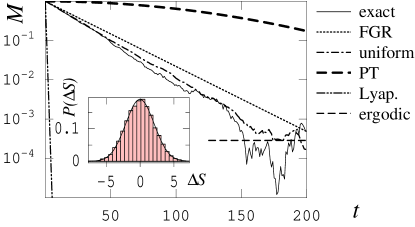
Figure 2: Fidelity in the FGR regime ($k=18$, $\lambda\approx 2.21$, $\epsilon=5\times 10^{-4}$, $n=3500$). Horizontal dashed line (“ergodic”) is the limit of FD due to the finite size of Hilbert space. Inset: Histogram of action differences compared to a Gaussian fit.

In the Lyapunov regime, FD is determined by dephasing of near trajectories with correlated actions JALABERT , invalidating simplification (11). Now the action difference $\Delta S^{\prime}\mathbf{-}\Delta S^{\prime\prime}$ depends on the initial momenta $p^{\prime}$, $p^{\prime\prime}$. Using reasoning similar to Ref. JALABERT or statistical arguments for a random walk with an exponentially increasing time step RANDOM_WALK , it can be shown that the action difference is also Gaussian distributed, with zero average and variance

$$\left\langle\left[\Delta S\left(p^{\prime}\right)-\Delta S\left(p^{\prime\prime}\right)\right]^{2}\right\rangle \approx(D/2\lambda)e^{2\lambda t}\left(p^{\prime}-p^{\prime\prime}\right)^{2},$$ (13)

$$D =2\int_{0}^{\infty}dt\,\left\langle V^{\prime}\left(0\right)V^{\prime}\left(t\right)\right\rangle.$$

We can therefore make the replacement

$$\left\langle\exp\left[\frac{i}{\hbar}(\Delta S^{\prime}\mathbf{-}\Delta S^{\prime\prime})\right]\right\rangle\approx\exp\left[-\frac{D}{4\lambda\hbar^{2}}e^{2\lambda t}\left(p^{\prime}-p^{\prime\prime}\right)^{2}\right]$$

in Eq. (9) and (10) to find

$$M_{L}\left(t\right)\approx\left(1+e^{2\lambda t}D/2\lambda\sigma^{2}\right)^{-1/2}\approx\left(2\lambda\sigma^{2}/D\right)^{1/2}e^{-\lambda t},$$

confirming Eq. (4). For the precise definition of $\lambda$, see Ref. SILVESTROV (one has to be careful about the averaging process). Fig. 3 displays $M\left(t\right)$ in the Lyapunov regime. It shows that while $M_{L}$ gives an accurate average decay only for $\lambda t\gg 1$, $M_{unif}$ correctly follows the behavior of $M_{exact}$ even for short times $t\sim\lambda^{-1}$. The inset shows the variance of $\Delta S\left(p^{\prime}\right)-\Delta S\left(p^{\prime\prime}\right)$ as a function of $p^{\prime}-p^{\prime\prime}$ at a fixed time and justifies the assumption made in Ref. JALABERT in derivation of perturbation independent decay: for near trajectories, the variance grows quadratically with $p^{\prime}-p^{\prime\prime}$ (fitted line gives an exponent 2.003), in accordance with Eq. (13), while for distant trajectories, in accordance with the derivation of the FGR regime, the variance is independent of $p^{\prime}-p^{\prime\prime}$,

$$\left\langle\left[\Delta S\left(p^{\prime}\right)-\Delta S\left(p^{\prime\prime}\right)\right]^{2}\right\rangle=2\sigma_{\Delta S}^{2}=4Kt.$$ (14)

Figure 3: Fidelity in the Lyapunov regime ($k=7$, $\lambda\approx 1.28$, $\epsilon=5\times 10^{-4}$, $n=10^{5}$). Meaning of lines same as in Fig. 2. Inset: Variance of $\Delta S\left(p^{\prime\prime}\right)-\Delta S\left(p^{\prime}\right)$ as a function of $p^{\prime\prime}-p^{\prime}$ at time $t=7$. Dots are numerically calculated, dashed line is the horizontal asymptote $2\sigma_{\Delta S}^{2}$, solid line is a linear fit for small $p^{\prime\prime}-p^{\prime\prime}$, in agreement with Eq. (13).

The time dependence of $\left\langle\left[\Delta S\left(p^{\prime}\right)-\Delta S\left(p^{\prime\prime}\right)\right]^{2}\right\rangle$ for fixed $p^{\prime}-p^{\prime\prime}$ is shown in Fig. 4. Part a) shows that for short times when trajectories are still correlated, this dependence is exponential, in agreement with Eq. (13). Part b) shows that for longer times, when correlation is lost, the dependence is linear, as expected from Eq. (14).

Figure 4: Variance of $\Delta S\left(p^{\prime\prime}\right)-\Delta S\left(p^{\prime}\right)$ as a function of $t$ for $p^{\prime\prime}-p^{\prime}=10^{-11}$: a) exponential dependence for short times, b) linear dependence for long times.

To conclude, we have explicitly evaluated SC expressions which were thought to be intractable numerically, yielding remarkably accurate results for FD in the FGR and Lyapunov regimes. We provided a more detailed explanation why CPA works and employed our method to test other approximations used in Refs. JALABERT ; CERRUTI .

This research was supported by the National Science Foundation under Grant No. NSF-CHE-0073544, by ITAMP at the Harvard-Smithsonian Center for Astrophysics, Harvard University, and by the Mathematical Sciences Research Institute at Berkeley. We would like to acknowledge helpful discussions with S. Tomsovic. E.J.H. acknowledges the hospitality of the Max Planck Institute for Complex Systems, Dresden and the Humboldt Foundation for hospitality and support.

References

- (1) A. Peres, Phys. Rev. A 30, 1610 (1984).
- (2) R.A. Jalabert and H.M. Pastawski, Phys. Rev. Lett. 86, 2490 (2001).
- (3) W.K. Rhim et al., Phys. Rev. Lett. 25, 218 (1970).
- (4) H.M. Pastawski et al., Phys. Rev. Lett. 75, 4310 (1995).
- (5) H.M. Pastawski et al., Physica 283A, 166 (2000).
- (6) F.M. Cucchietti et al., Phys. Rev. E 65, 046209 (2002).
- (7) N.R. Cerruti and S. Tomsovic, Phys. Rev. Lett. 88, 054103 (2002).
- (8) P. Jacquod, P.G. Silvestrov, and C.W.J. Beenakker, Phys. Rev. E 64, 055203 (2001).
- (9) J. Vaníček, Uniform semiclassical approximations and their applications, doctoral thesis, Harvard University, Cambridge, MA (2003).
- (10) P.G. Silvestrov, J. Tworzydlo, and C.W.J. Beenakker, Phys. Rev. E 67, 025204(R) (2003).
- (11) G. Benenti and G. Casati, Phys. Rev. E 65, 066205 (2002).
- (12) F.M. Cucchietti, H.M. Pastawski, and D.A. Wisniacki, Phys. Rev. E 65, 045206(R)(2002).
- (13) F.M. Cucchietti, D.A.R. Dalvit, J.P. Paz, and W.H. Zurek, quant-ph/0306142.
- (14) F.M. Cucchietti, H.M. Pastawski, and R.A. Jalabert, cond-mat/0307752.
- (15) T. Prosen, T.H. Seligman, and M. Ždinarič, quant-ph/0304104.
- (16) T. Prosen and M. Ždinarič, quant-ph/0306097.
- (17) M. Ždinarič and T. Prosen, J. Phys. A 36, 2463 (2003).
- (18) T. Prosen, Phys. Rev. E 65, 036208 (2002).
- (19) P. Jacquod, I. Adagideli, and C.W.J. Beenakker, Phys. Rev. Lett. 89, 154103 (2002).
- (20) P. Jacquod, I. Adagideli, and C.W.J. Beenakker, Europhys. Lett. 61, 729 (2003).
- (21) G. Benenti, G. Casati, and G. Veble, Phys. Rev. E 67, 055202(R) (2003).
- (22) B. Eckhardt, J. Phys. A 36, 371 (2003).
- (23) D.A. Wisniacki, E.G. Vergini, H.M. Pastawski, and F.M. Cucchietti, Phys. Rev. E 65, 055206(R) (2002).
- (24) D.A. Wisniacki and D. Cohen, Phys. Rev. E 66, 046209 (2002).
- (25) D.A. Wisniacki, Phys. Rev. E 67, 016205 (2003).
- (26) T. Kottos and D. Cohen, Europhys. Lett. 61, 431 (2003).
- (27) J. Emerson, Y.S. Weinstein, S.Lloyd, and D.G. Cory, Phys. Rev. Lett. 89, 284102 (2002).
- (28) Y.S. Weinstein, J. Emerson, S.Lloyd, and D.G. Cory, quant-ph/0201064 (2002).
- (29) Y. Adamov, I. V. Gornyi, and A.D. Mirlin, Phys. Rev. E 67, 056217 (2003).
- (30) W. Wang and B. Li, nlin.CD/0208013.
- (31) B. Georgeot and D.L. Shepelyansky, Eur. Phys. J. D 19, 263 (2002).
- (32) N.R. Cerruti and S. Tomsovic, J. Phys. A 36, 3451 (2003).
- (33) J. Vaníček and E.J. Heller, Phys. Rev. E 64, 026215 (2001).
- (34) J. Vaníček and E.J. Heller, Phys. Rev. E 67, 016211 (2003).
- (35) J. Vaníček and D. Cohen, J. Phys. A: Math. Gen. 36, 9591 (2003).
- (36) W.H. Miller, J. Chem. Phys., 53, 3578 (1970).
- (37) W.H. Miller, J. Phys. Chem. A 105, 2942 (2001).
- (38) J.H. Van Vleck, Proc. Natl. Acad. Sci. 14, 178 (1928).
- (39) S. Tomsovic and E.J. Heller, Phys. Rev. E 47, 282 (1993).
- (40) J. Vaníček and E.J. Heller (not published).