Suppression of Rabi oscillations for moving atoms

Abstract

The well-known laser-induced Rabi oscillations of a two-level atom are shown to be suppressed under certain conditions when the atom is entering a laser-illuminated region. For temporal Rabi oscillations the effect has two regimes: classical-like, at intermediate atomic velocities, and quantum at low velocities, associated respectively with the formation of incoherent or coherent internal states of the atom in the laser region. In the low velocity regime the laser projects the atom onto a pure internal state that can be controlled by detuning. Spatial Rabi oscillations are only suppressed in this low velocity, quantum regime.

I Introduction

The coupling between the center-of-mass motion of the atom and localized laser fields is a central topic in quantum optics, and leads to many important effects and applications in cooling, trapping, deflection, and isotope separation experiments. The objective of this paper is to point out one further consequence of such a coupling: the suppression of Rabi oscillations and the related possibility of controlled projection onto internal pure states by the motion of the atom from a laser-free region into a laser-illuminated region.

For a general two-level system with an interaction-picture Hamiltonian of the form

$$H=\frac{\hbar}{2}\left({0\atop\Omega}{\Omega\atop-2\delta}\right),$$ (1)

a state ${\bf\Psi}\equiv{\Psi^{(1)}\choose\Psi^{(2)}}$, beginning in the ground state $|1\rangle={1\choose 0}$ at $t=0$, will evolve according to

$$\Psi^{(1)} = e^{i\delta t/2}\left[\cos\left(\frac{\Omega^{\prime}t}{2}\right)-i\frac{\delta}{\Omega^{\prime}}\sin\left(\frac{\Omega^{\prime}t}{2}\right)\right],$$

$$\Psi^{(2)} = \frac{-ie^{i\delta t/2}\Omega}{\Omega^{\prime}}\sin\left(\frac{\Omega^{\prime}t}{2}\right),$$ (2)

where

$$\Omega^{\prime}=(\Omega^{2}+\delta^{2})^{1/2}$$ (3)

and $\Omega$ is the usual Rabi frequency.

There is currently much interest in the dynamics of two-level systems governed by the Hamiltonian of Eq. (1) plus an additional time-dependent driving term, in particular to determine the Rabi oscillation suppression for critical values of the external field parameters. In the so called dynamical localization effect, for example, the system remains in one of the two levels Sacchetti01 . Another Rabi-oscillation-suppression effect has been described recently for the scattering of atoms by a standing light wave EFYS02 . In this case, the partial contributions from different diffraction angles lead to different oscillation periods and thus to inhomogeneous broadening.

In this paper we describe a different type of oscillation suppression due to the motion of the system rather than to an additional time dependent field, or to a diffraction effect. Explicitly, we shall consider the motion of a two-level atom with transition frequency $\omega$ in one dimension, with a classical electric field (laser of frequency $\omega_{L}$) illuminating the half axis $x>0$ perpendicularly. Without damping, and in an interaction picture for the internal degrees of freedom, the Hamiltonian can be written in the form

$$H=\hat{p}^{2}/2m+\frac{\hbar}{2}\left({0\atop\Omega\Theta(\hat{x})}{\Omega\Theta(\hat{x})\atop-2\delta}\right),$$ (4)

where $\Theta$ is the step function, $\Omega$ plays the role of a laser-atom coupling constant, $\delta=\omega_{L}-\omega$ is the detuning, and hats denote operators whenever confusion is possible with a corresponding $c$-number. In particular, $\hat{p}$ is the momentum operator for the $x$ direction. If one takes damping due to photon emissions into account, it can be shown, by means of the quantum jump approach Hegerfeldt91 , that in three dimensions the atomic time development between emissions may be described by an (effective, non-hermitian) “conditional” Hamiltonian $H_{\rm c}$,

$$H_{\rm c} = {\bf{\hat{p}}}^{2}/2m+\frac{\hbar}{2}\Omega\,\Theta(\hat{x})\left\{|2\rangle\langle 1|e^{ik_{L}\hat{y}}+{\rm h.c.}\right\}$$ (5)

$$- \frac{\hbar}{2}(2\delta+i\gamma)|2\rangle\langle 2|,$$

where $\gamma$ is the Einstein coefficient of level 2, i.e. its decay rate or inverse life time, and ${\bf{\hat{p}}}$ is the momentum operator in three dimensions (3D). The factor $e^{ik_{L}\hat{y}}$ takes into account the spatial dependence of the laser coupling. A Hamiltonian of the form of Eq. (4) is obtained from Eq. (5) by neglecting spontaneous emissions, i.e. setting $\gamma=0$, and assuming in addition that the atomic wave packet is centered at $y=0$ and satisfies $k_{L}\Delta y\ll 1$, at least for some time, so that the exponentials can be dropped and a one dimensional kinetic term suffices. This approximation and its limitations will be further commented on Appendix A.

The conditional Hamiltonian $H_{\rm c}$ is closely related to waiting times between photon emissions Cohen-Dalibard85 . Indeed, let an atomic state $|\Psi(0)\rangle$ be prepared at time $0$. Then it can be shown by means of the quantum jump approach Hegerfeldt91 that

$$P_{0}(t)\equiv||e^{-iH_{\rm c}(t)/\hbar}|\Psi(0)\rangle||^{2}$$ (6)

gives the probability of no emission until time $t$ and $\Pi(t)\equiv-P_{0}^{\prime}(t)$ is the probability density for the first photon. After an emission the atom has to be reset, here to its ground state, and then the conditional time development resumes. In this way one can simulate an emission sequence and the corresponding Bloch (master) equation for the atom.

As we will show, for moving atoms there are Rabi oscillations both in time as well as in space. In the temporal case one asks for the probability, $P_{2}(t)$, of finding the atom in the excited state, without regard to its spatial position. For the simple model in Eq. (4) without damping, this can be easily calculated and Figure 1 depicts a suppression for this case. The solid line shows the population of the excited state $P_{2}$ versus $t$ for $\delta=0$ and for a wave packet which is prepared at $t=0$ with negligible negative momentum components as a minimum-uncertainty-product Gaussian, with the atom in the ground state, and far from the laser. At sufficiently large times, and for the parameters we have chosen, the wave packet is completely within the laser region, but there are no Rabi oscillations. Instead, $P_{2}$ increases monotonically, and saturates at $0.5$; this might look surprising at first sight: there is no classical averaging (the state is quantum and coherent), there is no dispersion related broadening, there is no time dependent term in the Hamiltonian, there is not even decay that could smooth or suppress the oscillation.

Figure 1: Probability of excited state $P_{2}$ versus $t-t_{0}$, where $t_{0}$ is a mean entrance time, see the definition below. $\Omega=166.5\times 10^{6}$ s^-1, $\gamma=\delta=0$. The initial states (at $t=0$) for the center of mass are minimum-uncertainty product Gaussians with $\Delta_{x}=0.24\,\mu$m, $\langle x\rangle=-1.32\,\mu$m, and $\langle v\rangle=9.03$ m/s (solid line), 49.68 m/s (dotted line) and 36.13 m/s (dashed line). $t_{0}=-\langle x\rangle/\langle v\rangle$. The atomic mass is taken to be that of Cs here and in all following figures.

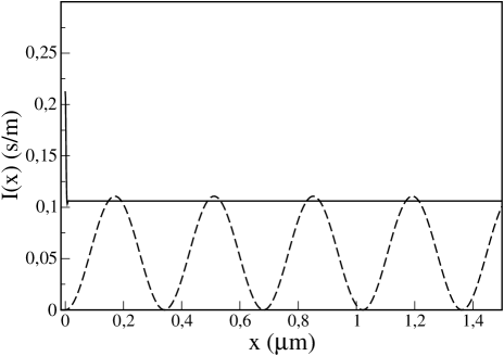
Figure 2: Probability density of the excited state, integrated over time, for two different wave packets: $\langle v\rangle=0.0090$ m/s (solid line) and $\langle v\rangle=9.03$ m/s (dashed line); $\Omega=166.5\times 10^{6}$ s^-1; $\gamma=\delta=0$. The initial state is a minimum-uncertainty-product Gaussian in the ground state with $\Delta_{x}=0.24\,\mu$m, and $\langle x\rangle=-1.32\mu$m. With these parameters $v_{c}=k_{c}\hbar/m=0.28$ m/s and $v_{R}=k_{R}\hbar/m=32.3$ m/s, see Eqs. (22) and (25).

Basically, for measurements in time the effect has two different regimes and explanations depending on the incident energy: at very low kinetic energy, the suppression is due to the formation of a pure non-oscillating internal state of the atom in the laser region, whereas at intermediate energies it may be understood in terms of a simple semiclassical approximation. Yet at higher energies the effect disappears, and the expected Rabi oscillations may be seen more and more clearly for increasing velocities, as illustrated by the dashed and dotted lines of Figure 1.

Spatial Rabi oscillations can occur in the emission probability at different atomic positions. If $P_{2}(x,t)$ denotes the probability density to find the atom in its excited state at the position $x$ at time $t$ and if one defines $I(x)$ by

$$I(x)\equiv\int dtP_{2}(x,t),$$ (7)

then $\gamma I(x)dx$ gives the number of emitted photons (per atom) with the atom at $dx$, and thus $I(x)$ is proportional to the photon intensity for the atom at position $x$ foot1 . Neglecting damping, the expression on the rhs can be calculated with Eq. (4), and an example is given in Fig. 2, where the spatial Rabi oscillation is completely absent in one of the two cases depicted. In contrast to the temporal case, spatial oscillations are only suppressed by the quantum mechanism, i.e., at very low kinetic energies.

In the next four sections we shall characterize, neglecting damping due to spontaneous emissions, several aspects of the Rabi oscillation suppression due to atomic motion: the basic theory (Section II), the effect of the velocity regimes in the Rabi oscillations for measurements in time (Section III), the effect of detuning and the velocity in the internal atomic states (Section IV), and the suppression of spatial Rabi oscillations (Section V). The effect of damping will be taken into account in Section VI.

II Basic theory

II.1 Exact results

Here we shall present the theory required to describe the interaction of the moving atom with the perpendicular laser. We first neglect damping and solve the eigenvalue equation for the Hamiltonian of Eq. (4) subject to the condition that the atom impinges on the laser beam from the left in the ground state. The eigenvalues are $E=\hbar^{2}k^{2}/2m$ and the eigenfunctions are denoted by ${\bf\Phi}_{k}\equiv{\phi^{(1)}\choose\phi^{(2)}}$, with $k>0$.

For $x\leq 0$, ${\bf\Phi}_{k}$ is of the form

$${\bf\Phi}_{k}(x)=\frac{1}{\sqrt{2\pi}}\left({e^{ikx}+R_{1}e^{-ikx}\atop R_{2}e^{-iqx}}\right),\quad x\leq 0,\quad k>0,$$ (8)

where

$$q^{2}=k^{2}+2m\delta/\hbar$$ (9)

and ${\rm{Im}}(q)\geq 0$. For large enough (negative) detuning, $k<|2m\delta/\hbar|^{1/2}$, $q$ becomes purely imaginary and the reflected wave for the excited state decays exponentially.

In the laser region, let $|\lambda_{+}\rangle$ and $|\lambda_{-}\rangle$ be the eigenstates of the matrix $\frac{1}{2}\left({0\atop\Omega}{\Omega\atop-2\delta}\right)$ corresponding to the eigenvalues $\lambda_{\pm}$. One easily finds

$$\lambda_{\pm} = -\frac{1}{2}[\delta\pm\Omega^{\prime}],$$ (10)

$$|\lambda_{\pm}\rangle = {1\choose\frac{-(\delta\pm\Omega^{\prime})}{\Omega}}.$$ (11)

Note that $|\lambda_{\pm}\rangle$ have not been normalized.

For $x\geq 0$, one can write ${\bf\Phi}_{k}$ as a superposition of $|\lambda_{\pm}\rangle$,

$$\sqrt{2\pi}{\bf\Phi}_{k}(x)=C_{+}|\lambda_{+}\rangle e^{ik_{+}x}+C_{-}|\lambda_{-}\rangle e^{ik_{-}x}.$$ (12)

[The mathematical solutions $e^{-ik_{\pm}x}$ are not included because they correspond to negative momenta or increasing exponentials.]

From the eigenvalue equation $H{\bf\Phi}_{k}=E_{k}{\bf\Phi}_{k}$ it follows that

$$k_{\pm}^{2}=k^{2}-2m\lambda_{\pm}/\hbar=k^{2}+\frac{m}{\hbar}(\delta\pm\Omega^{\prime}),$$

with Im $\,k_{\pm}\geq 0$, and from the continuity of ${\bf\Phi}_{k}(x)$ at $x=0$ one obtains, with $|1\rangle={1\choose 0}$ and $|2\rangle={0\choose 1}$,

$$1+R_{1} = C_{+}\langle 1|\lambda_{+}\rangle+C_{-}\langle 1|\lambda_{-}\rangle$$

$$R_{2} = C_{+}\langle 2|\lambda_{+}\rangle+C_{-}\langle 2|\lambda_{-}\rangle.$$

Similar relations result from the continuity of ${\bf\Phi}_{k}^{\prime}(x)$ at $x=0$, yielding

$$C_{+} = -2k(q+k_{-})\lambda_{-}/D,$$

$$C_{-} = 2k(q+k_{+})\lambda_{+}/D,$$

$$R_{1} = [\lambda_{+}(q+k_{+})(k-k_{-})-\lambda_{-}(q+k_{-})(k-k_{+})]/D,$$

$$R_{2} = k(k_{-}-k_{+})\Omega/D,$$ (13)

where

$$D=(k+k_{-})(q+k_{+})\lambda_{+}-(k+k_{+})(q+k_{-})\lambda_{-}.$$ (14)

Thus Eq. (12) becomes, in components and for $x\geq 0$,

$$\phi_{k}^{(1)}(x) = -\frac{2k}{\sqrt{2\pi}D}\{(q+k_{-})\lambda_{-}e^{ik_{+}x}-(q+k_{+})\lambda_{+}e^{ik_{-}x}\},$$

$$\phi_{k}^{(2)}(x) = \frac{k\Omega}{\sqrt{2\pi}D}\{(q+k_{-})e^{ik_{+}x}-(q+k_{+})e^{ik_{-}x}\}.$$ (15)

Time dependent wave packets incident on the laser region with positive momentum components and with the atom in the ground state may be formed by linear superposition DEHM02 ,

$${\bf\Psi}(x,t)=\int_{0}^{\infty}dk\,e^{-i\hbar k^{2}t/2m}{\bf\Phi}_{k}(x)\tilde{\psi}(k),$$ (16)

where $\tilde{\psi}(k)$ is the wave number amplitude at time $t=0$ corresponding to the freely moving packet.

The conditional Hamiltonian $H_{c}$ for the one-dimensional case with damping can be treated in a similar way, and this is done in Appendix B.

II.2 Different approximation regimes

Depending on the incident velocity different approximations are applicable. For large velocities a semiclassical approximation is sufficient whereas for slow atoms it is essential to retain the quantum nature of the translational motion.

II.2.1 Fast atoms: semiclassical approximation

For “high” kinetic energy, $k^{2}\gg|m(\delta\pm\Omega^{\prime})/\hbar|$, we may approximate the wave numbers in the wave function by

$$k_{\pm} \approx k+\frac{m}{2\hbar k}[\delta\pm\Omega^{\prime}],$$ (17)

$$q \approx k+\frac{m\delta}{k\hbar},$$ (18)

and therefore,

$$\phi_{k}^{(1)}(x) \approx \frac{e^{ikx}}{\sqrt{2\pi}}\bigg{\{}e^{i\delta t/2}\bigg{[}\cos\left(\frac{m\Omega^{\prime}x}{2\hbar k}\right)$$

$$- i\frac{\delta}{\Omega^{\prime}}\sin\left(\frac{m\Omega^{\prime}x}{2\hbar k}\right)\bigg{]}\bigg{\}},$$

$$\phi_{k}^{(2)}(x) \approx \frac{e^{ikx}}{\sqrt{2\pi}}\bigg{\{}e^{i\delta t/2}\bigg{[}\frac{-i\Omega}{\Omega^{\prime}}\sin\left(\frac{m\Omega^{\prime}x}{2\hbar k}\right)\bigg{]}\bigg{\}}.$$ (19)

[The relation with the Raman-Nath approximation is discussed in Appendix C.] Up to the normalization factor this reveals a “spatial Rabi oscillation” that may be associated with the temporal one by the change of variable $t=xm/k\hbar$, the time that a classical particle with momentum $k\hbar$ needs to travel from the origin to $x$. With this change the terms in curly brackets correspond exactly to the internal state amplitudes of the atom at rest, see Eq. (2), while the multiplying plane wave denotes an undisturbed center of mass motion with fixed momentum.

Moreover in this regime reflection is negligible,

$$R_{1}\approx\left(\frac{m\Omega}{4\hbar k^{2}}\right)^{2},\;\;\;R_{2}\approx\frac{m\Omega}{4\hbar k^{2}}.$$ (20)

Figure 3: Densities for ground (solid line) and excited state (dashed line) at $t=0.5\,\mu$s. The initial state (at $t=0$) is a minimum-uncertainty product Gaussian for the center of mass, with $\Delta_{x}=0.2436\,\mu$m, $\langle x\rangle=-1.32\,\mu$m, and $\langle v\rangle=9.03$ m/s; $P_{2}(t=0)=0$; $\Omega=166.5\times 10^{6}$ s^-1, $\gamma=\delta=0$, and the mass corresponds to a Cs atom.

A further simplification is to assume that the interferences among different momenta are either negligible or average out. Then we may quite accurately approximate the center of mass motion of a wave packet with high kinetic energy by a purely classical free motion, whereas the internal state is treated quantum mechanically. More specifically, in this approximation the wave packet width and spreading are taken into account by using an ensemble of semiclassical atoms with their center of mass distributed in classical phase space according to the initial quantum Wigner function $W(q_{0},p_{0};t=0)$. [For free motion, the quantum and “classically evolved” Wigner functions coincide at all times if initially identical.] To each of these atoms we associate an internal state, that starts to oscillate once the center of mass crosses $x=0$ at $-q_{0}m/p_{0}$. The expectation values in the semiclassical approximation are then computed by averaging over the ensemble of semiclassical atoms (translationally classical, internally quantum). In particular, the probability to find the atom in the excited state at a time $t$ is given by

$$P_{2}(t) = \int_{-\infty}^{\infty}dq_{0}\int_{0}^{\infty}dp_{0}\,W(q_{0},p_{0};t=0)$$

$$\times \left(\frac{\Omega}{\Omega^{\prime}}\right)^{2}\sin^{2}[\Omega^{\prime}(t+q_{0}m/p_{0})/2]\Theta(t+q_{0}m/p_{0}),$$

where we have assumed that $t>0$, that the wave packet at $t=0$ is far from the laser, and that all atoms have positive momentum.

II.2.2 Slow atoms

At the critical wavenumber $k=k_{c}$,

$$k_{c}\equiv[m(\Omega^{\prime}-\delta)/\hbar]^{1/2},$$ (22)

the de Broglie wavelength for the atomic motion $\lambda_{dB}(k)=2\pi/k$ becomes equal to the “spatial period” of the Rabi oscillation in Eq. (19), or “Rabi wavelength” $\lambda_{R}(k)=2\pi k/k_{c}^{2}$. For smaller $k$ the quantum aspect of the atomic motion cannot be ignored, and $k_{-}$ becomes purely imaginary,

$$k_{-}\approx ik_{c},$$ (23)

whereas $k_{+}$ remains real. As a consequence, $e^{ik_{-}x}$ evanesces, and the contribution of $|\lambda_{-}\rangle$ beyond $k_{c}^{-1}$ (the penetration length for this component) vanishes,

$$\phi_{k}^{(1)}(x) \approx \frac{C_{+}}{\sqrt{2\pi}}e^{ik_{+}x},\;\;\;x>k_{c}^{-1}$$ (24)

$$\phi_{k}^{(2)}(x) \approx -\frac{C_{+}(\delta+\Omega^{\prime})}{\sqrt{2\pi}\Omega}e^{ik_{+}x},\;\;\;x>k_{c}^{-1}.$$

This results in a pure, and non-oscillating internal state, as discussed later in Section IV.

III Temporal Rabi oscillations: velocity effects

In addition to the separation between “classical” and “quantum” regimes at $k_{c}$, see Eq. (22), the classical regime may be also subdivided into intermediate and high velocities, depending on whether or not the temporal Rabi oscillations are suppressed. (We shall see later than for spatial oscillations this later subdivision does not apply.)

III.1 High velocities: $\langle k\rangle>k_{R}$

Suppose that the center of mass motion of the wave packet can be reproduced with an ensemble of classical atoms, as discussed in the previous section, and that they enter into the laser region in a very short time compared to the the Rabi period $T_{R}\equiv 2\pi/\Omega^{\prime}$ (sudden entrance). In that case they will oscillate in phase and the Rabi oscillations will be seen, as in the dotted line of Figure 1. For Gaussian packets, the transition (average) wave number between adiabatic and sudden entrance regimes may be identified by equating $T_{R}$ and a measure of the duration of the wave packet passage across the origin, $t_{p}\approx 5\Delta_{x}m/\langle k\rangle\hbar$, where $\Delta_{x}$ is the wave packet width (square root of variance) at the peak’s passage across $x=0$, and the factor 5 is rather arbitrary but is only intended to give an estimate,

$$k_{R}\approx\frac{5\Delta_{x}m\Omega^{\prime}}{2\pi\hbar}.$$ (25)

III.2 Intermediate velocities: $k_{c}<\langle k\rangle<k_{R}$

In the intuitive language suggested by the classical approximation for the center of mass motion, the “mechanism” that explains the suppression of temporal Rabi oscillations at intermediate velocities is the averaging of the Rabi oscillations of the individual atoms forming the ensemble when the entrance time for the whole ensemble is long compared to the Rabi period. Since each atom enters at a different instant in the laser region, the phase of the oscillation will be also different. This is the case shown in Fig. 3, where the peaks of the densities of the ground and excited state alternate with a spatial period given by $\hbar\langle k\rangle T_{R}/m$.

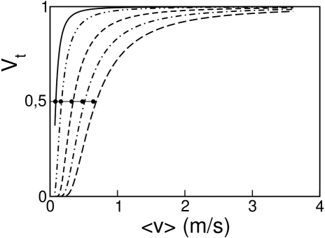
Figure 4: Visibilities, Eq. (26) (the quantum and semi-classical results are indistinguishable in the scale of the figure) for (from left to right) $\Omega=0.413,\,0.827,\,1.654,\,2.480,$ and $3.307$ $\times 10^{6}$ s^-1. In all cases the initial Gaussian has $\Delta_{x}=0.2438\,\mu$m, $\langle x\rangle=-1.32\,\mu$m, and $\gamma=\delta=0$. Also drawn are the corresponding values of the transition velocities $v_{R}=k_{R}\hbar/m$ with circles.

Figure 4 shows the “visibility” $V_{t}$ obtained from maxima (max) and minima (min) of the probability of the excited state, $P_{2}(t)$, corresponding to large times beyond the initial transient,

$$V_{t}=\frac{P_{2}(max)-P_{2}(min)}{P_{2}(max)+P_{2}(min)},$$ (26)

versus the incident average velocity for five different values of $\Omega$ and a fixed wave packet width, as well as the estimate given by Eq. (25); again $\delta=0$. The visibilities calculated exactly or with the classical approximation are indistinguishable.

III.3 Low velocity: $\langle k\rangle<k_{c}$

Below $k_{c}$ there are no Rabi oscillations either but, according to the discussion of section II.2.2, the reason is not an effective “averaging” (the semiclassical approximation is not valid), but the fact that the atomic internal state formed by the laser does not oscillate at all.

IV Internal states: Effects of the velocity and detuning

The motion of the atom from the laser-free region to the laser-illuminated region has very different effects on the internal state depending on the incident velocity and the detuning. We shall discuss now the effect of the various velocity regimes in the degree of mixing of the normalized, internal, reduced density operator for the atoms in the laser region, which is defined by its matrix elements

$$\rho^{L}_{ij}(t)=\frac{\int_{0}^{\infty}dx\,[\psi^{(i)}(x,t)]^{*}\psi^{(j)}(x,t)}{\int_{0}^{\infty}dx\,|\psi^{(1)}(x,t)|^{2}+|\psi^{(2)}(x,t)|^{2}},$$ (27)

distinguishing between the cases of zero and non-zero detuning.

IV.1 Zero detuning

(i) For $\langle k\rangle<k_{c}$ the populations of both ground and excited states are equal and the overlap in space of the respective wave functions is maximum. After a transient time, necessary for Eq. (24) to apply, $\rho^{L}$ is finally given by the pure state $2^{-1/2}(|1\rangle-|2\rangle)$,

$$\rho^{L}=\left({1/2\atop{-1/2}}{{-1/2}\atop 1/2}\right),$$ (28)

which is nothing but $|\lambda_{+}\rangle\langle\lambda_{+}|$, now normalized.

(ii) For $k_{c}<k<k_{R}$ excited and ground components do not overlap, see Fig. 3, so $\rho^{L}$ tends to a diagonal matrix. The two populations are still equal (there is no global Rabi oscillation because of the semiclassical averaging effect) and $\rho^{L}$ is 1/2 times the unit matrix, which amounts to the maximum degree of mixing (incoherence) allowed for the reduced internal state. The sharp transition from a pure state to a maximally mixed state around $\langle k\rangle=k_{c}$ may be seen in Figure 5.

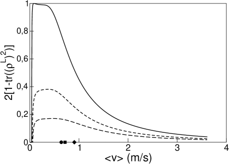
Figure 5: Degree of mixing versus $\langle v\rangle$ for $\gamma=0$, $\Omega=3.3\times 10^{6}$ s^-1, $\langle x\rangle=-1.34\,\mu$m, and $\Delta_{x}=0.2436\,\mu$m. $\delta=0$ (solid line), $-\Omega/2$ (short dashed line) and $-\Omega$ (long dashed line). Also marked are the corresponding values of $\hbar k_{R}/m$ (circle, square and diamond respectively).

There is also quite a dramatic effect of $k_{c}$ on the reflection probabilities, which tend to vanish for higher values of $k$, see Figures 6 and 7 for $|R_{1}|^{2}$ and $|R_{2}|^{2}$ respectively.

Figure 6: Reflection probability to the ground state versus $v$ for $\Omega=166.5\times 10^{6}$ s^-1; $\gamma=0$; $\delta=$ $-\Omega/4$ (dotted-dashed line), $0$ (solid line), and $\Omega/4$ (dashed line). $\hbar k_{c}/m$ is indicated with a circle, square and diamond respectively.

Figure 7: Reflection probability to the excited state versus $v$ for $\Omega=166.5\times 10^{6}$ s^-1; $\gamma=0$; $\delta=$ $\Omega/4$ (dashed line), $0$ (solid line), and $-\Omega/4$ (dotted-dashed line). $\hbar k_{c}/m$ is indicated with a circle, square and diamond respectively. The peak close to $0.2$ is at the point where $q$ passes from imaginary to real.

(iii) Finally, for $k\gg k_{R}$ there is no classical averaging effect, and the two populations oscillate periodically and coherently in time between 0 and 1. The reduced internal state in the laser region becomes pure again, as Figure 5 shows. Note that the transition from intermediate to high kinetic energies at $k_{R}$ is rather smooth, in particular in comparison with the sharp $k_{c}$-transition.

If the initial atom is prepared in the excited state instead of the ground state, different scattering eigenfunctions have to be used. The calculation follows similar lines and provides different expressions for reflection amplitudes and coefficients $C_{\pm}$. However, the eigenstates $|\lambda_{\pm}\rangle$ remain the same, and it is still true that below $k=k_{c}$ only $k_{+}$ is real, so that the same pure state is obtained at low kinetic energy. This means that the low-energy motion of the atom into a laser illuminated region provides a very simple physical mechanism to project any initial internal state, pure or mixed, onto the pure state $2^{-1/2}(|1\rangle-|2\rangle)$ if $\delta=0$. The laser illuminated region may in fact be moved and the atom be at rest with the same effect.

IV.2 Non-zero detuning

Detuning may be used as a control knob to obtain states with a smaller fraction of excited state. The (unnormalized) pure state obtained at low kinetic energy in the laser region is given for arbitrary $\delta$ by

$${\bf\Psi}={1\choose-\frac{\delta+\Omega^{\prime}}{\Omega}}.$$ (29)

As seen in Figure 5, for the intermediate regime $k_{c}<\langle k\rangle<k_{R}$, the classical averaging is not so effective for non zero detuning, so that the state is less mixed. Note also that negative detuning leads to less reflection at very low kinetic energies than positive detuning, see Figs. 6 and 7, and the existence of an additional critical point associated with the transition between imaginary and real values of $q$.

V Suppression of spatial Rabi oscillations

The quantum suppression of Rabi oscillations below $k_{c}$ may also be seen in several space dependent quantities. They are, however, not sensitive at all to the semiclassical mechanism: these quantities oscillate both below and above $k_{R}$ defined in Eq (25).

In Figure 8 we show

$$V_{x}=\frac{|\phi_{k}^{(2)}(x)|^{2}(max)-|\phi_{k}^{(2)}(x)|^{2}(min)}{|\phi_{k}^{(2)}(x)|^{2}(max)+|\phi_{k}^{(2)}(x)|^{2}(min)}$$ (30)

for maxima and minima with respect to $x$ evaluated beyond the penetration length of the $\lambda_{-}$-component. One may see a rather abrupt jump from 0 to 1 at $k=k_{c}$.

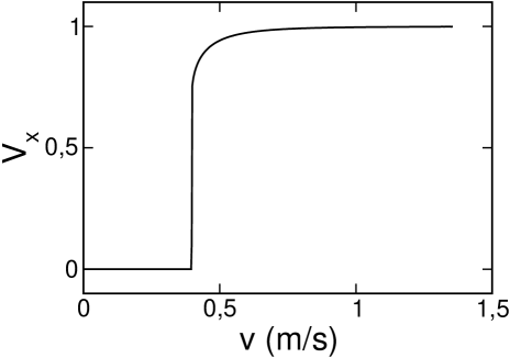
Figure 8: Spatial visibility, Eq. (30), versus $v$ for $\Omega=3.307\times 10^{6}$ s^-1, $\gamma=0$, and $\delta=0$.

A similar jump may be observed for $I(x)$ of Eq. (7). For wave packets with components below $k_{c}$, so that $k_{+}\approx k_{c},\,k_{-}\approx ik_{c}$, and for $x$ beyond the transient, small-$x$ region, the $t$ integral can be done to obtain $I(x)\approx\langle v\rangle/v_{c}^{2}$. On the other hand, for $k$ above $k_{c}$, $I(x)$ becomes

$$I(x)\approx\frac{m}{\hbar}\int_{0}^{\infty}\,\frac{dk}{k}\sin^{2}\left(\frac{\Omega x}{2v}\right)|\langle k|\psi^{(1)}(0)\rangle|^{2}.$$ (31)

These two limiting cases are depicted in Figure 2.

VI Inclusion of Damping

In this section we shall see that the suppression of Rabi oscillations can be detected by means of the fluorescence signal of the spontaneously emitted photons. Two cases will be considered: a detection measurement of the first fluorescence photon, which is described by the conditional Hamiltonian, and a measurement where all successive photons are also taken into account, which requires a master equation (optical Bloch equations). In both cases the fluorescence signal is proportional to the population of the excited state $P_{2}$ which can be calculated by means of $H_{c}$ or by the Bloch equations, respectively.

Figure 9: Fading (not suppression!) of Rabi oscillations for an atom at rest: $P_{2}$ versus $t$ for $\gamma=33.3\times 10^{6}$ s^-1, $\Omega=5\gamma$, $\delta=0$. The solid line corresponds to the master equation and the dashed one to the conditional Hamiltonian (“first photon”).

The suppression of Rabi oscillations discussed here should be distinguished from their fading away due to damping and approach to a stationary internal state. The latter is quite well-known for atoms at rest WM (cf. Figure 9). It is possible to operationally distinguish fading and suppression by a combination of $\Omega$ and $\gamma$ that, for the atom at rest, allows to observe several oscillations before reaching the asymptotic stationary population. This corresponds to strong driving conditions, $\Omega\gg\gamma$.

VI.1 Rabi oscillations in the first-photon distribution

For the one-dimensional case the conditional Hamiltonian $H_{c}$ can be written as

$$H_{c}=\frac{\hat{p}^{2}}{2m}+\frac{\hbar}{2}\left({0\atop\Omega\Theta(\hat{x})e^{ik_{L}y}}{\Omega\Theta(\hat{x})e^{-ik_{L}y}\atop-2\delta-i\gamma}\right).$$ (32)

The generalization of Eqs. (11-14) for $\gamma\neq 0$ is provided in Appendix B.

For high velocities the entrance of the wave packet in the laser region is sudden, so that $P_{2}$ versus time takes the same form as for the atom at rest from the entrance time on. At lower velocities the oscillation pattern disappears; $k_{R}$ still marks the transition, which is now smoother than when $\gamma=0$. Figure 10 shows $P_{2}$ for a velocity below $k_{R}$. The Rabi oscillation suppression is evident, compare with the dashed line of Figure 9.

The transition at $k_{c}$ is illustrated in Fig. 11, which shows the degree of mixing versus the average velocity foot2 . Note the smoothing effect of a non-zero $\gamma$.

An observation of the suppression of Rabi oscillations using the first photon could be achieved for a “Lambda” configuration of three atomic levels such that the laser couples two of them, while a third one acts as a sink for the excited state EFYS02 (only one photon may be emitted per atom). The ideal experiment would require a preparation of the atoms, sent one by one, according to a single wave function, and a detector capable of responding to a single photon. The experiment would be repeated many times until a profile similar to the one in Fig. 10 is obtained for the density of photon detection times.

Figure 10: $P_{2}$ versus $t$ for $\gamma=33.3\times 10^{6}$ s^-1, $\Omega=5\gamma$ and $\delta=0$. The parameters of the initial Gaussian are $\langle v\rangle=9,03$ m/s, $\Delta_{x}=0.2436$ $\mu$m, and $\langle x\rangle=-1.322$ $\mu$m.

Figure 11: Degree of mixing of the internal state in the laser region versus $\langle v\rangle$ for $\Delta_{x}$= 0.2436 $\mu$m, $\gamma=33.3\times 10^{6}$ s^-1, $\Omega=10\gamma$ (solid line), and $\Omega=5\gamma$ (dashed line). The corresponding values of $\hbar k_{c}/m$ are also shown with a circle and a square respectively.

VI.2 Temporal Rabi oscillations in the photon intensity

For a simple two-level atomic configuration, without a sink level for the excited state, the atom may emit many photons. In this case recoil effects may become important, especially at low incident energies, and lead to spatial broadening. The master equation that describes the density operator $\rho^{3D}$ of the atomic system in three spatial dimensions is given, following Hegerfeldt93 , by

$$\dot{\rho}^{3D}=-\frac{i}{\hbar}\{H_{c}\rho^{3D}-\rho^{3D}H_{c}^{\dagger}\}+{\cal R}(\rho^{3D}),$$ (33)

where $H_{c}$ is the conditional 3D Hamiltonian, Eq. (5), and the “reset” or “jump” term ${\cal R}(\rho^{3D})$ takes into account the atomic recoil along the directions weighted by the dipole emission distribution. In momentum representation,

$$\langle{\bf p}|{\cal R}(\rho^{3D})|{\bf{p}}^{\prime}\rangle = \gamma|1\rangle\langle 1|$$

$$\times \int d{\bm{\kappa}}P(\bm{\kappa})\langle{\bf{p}}+\hbar k_{L}{\bm{\kappa}}|\rho^{3D}_{22}|{\bf p}^{\prime}+\hbar k_{L}{\bm{\kappa}}\rangle,$$

where the integral is over all possible photon directions represented by the unit vectors $\bm{\kappa}={\bf k}/|{\bf k}|$, and

$$P({\bm{\kappa}})=\frac{3}{8\pi}\left(1-\frac{{\bm{\kappa}}\cdot{\bf d}}{|{\bf d}|^{2}}\right)=\frac{3}{8\pi}\sin^{2}\theta,$$ (35)

$\theta$ being the angle between ${\bm{\kappa}}$ and the dipole moment ${\bf d}$, which is taken along the $z$ direction.

Even though the fluorescence photons and the associated atom recoil may go in any direction, one can take the trace over momentum components $p_{y}$ and $p_{z}$ in the reset term, and reduce the integral to a one dimensional one, see e.g. Hensinger01 , to obtain for the initial atomic-motion direction $x$ the expression

$${\cal R}_{x}(\rho) \equiv {\rm Tr}_{y,z}{\cal R}(\rho^{3D})=|1\rangle\langle 1|\gamma\frac{3}{8}$$

$$\times \int_{-1}^{1}du\,(1+u^{2})\langle p_{x}+\hbar k_{L}u|\rho_{22}|p^{\prime}_{x}+\hbar k_{L}u\rangle,$$

where the reduced atomic density operator for the $x$-direction is

$$\rho_{ij}\equiv{\rm Tr}_{y,z}\langle i|\rho^{3D}|j\rangle,\;\;i=1,2,\;\;j=1,2.$$ (37)

Note that it contains both internal and center of mass information of the atom, so it is different from $\rho^{L}$ in Eq. (27). Even though, taking the trace over $y$ and $z$ in the other terms of Eq. (33) does not lead to a closed equation for the reduced one-dimensional density matrix of Eq. (37), a one-dimensional approximation is valid,

$$\dot{\rho}=-\frac{i}{\hbar}\{H_{c}\rho-\rho H_{c}^{\dagger}\}+{\cal R}_{x}(\rho),$$ (38)

with $H_{c}$ given by Eq. (32), provided that the effect of the two broadening mechanisms in the $y$ direction, the standard quantum mechanical wave packet spreading and the atomic recoil, remain small. The time scales of both effects are estimated in Appendix A.

The fluorescence signal is proportional to $P_{2}$, which is now the total population of excited atoms, regardless of whether or not they have emitted. The one dimensional master equation may be solved in principle directly, or, as done here, using the quantum jump technique, i.e., averaging over many “trajectories” Hegerfeldt91 . For each of them the photon detections occur at random instants. Figure 12 shows $P_{2}$ averaged over 10000 trajectories, compared with the solid line of Figure 9, properly shifted, which gives the time evolution of $P_{2}$ for a sudden entrance of a very fast wave packet. The suppression of Rabi oscillations is evident.

The ideal fluorescence measurement would be performed by sending one atom at a time, as described before. In a less demanding experiment, one could prepare a cloud of many atoms of sufficiently low density, and send it towards the laser, measuring the fluorescence signal versus time. The cloud ensemble would lead to suppression of Rabi oscillations at sufficiently low velocities. In this case the incident translational state would not be pure but a true mixture.

The transition at $k_{c}$ would be most easily noticed by the reflection dominant at lower kinetic energies. For the Cs transition we are considering in the numerical examples $v_{c}\equiv\hbar k_{c}/m=0.28$ m/s, which is well above the recoil velocity limit $\hbar k_{L}/m=0.35$ cm/s. The possibility to control the pure state formed in the laser region will depend on the ability to focus the atomic beam along the $y$- direction in the scale of the laser wavelength, due to the $y$-dependence of the pure state obtained, see Eq. (48).

Figure 12: $P_{2}$ versus time for $\gamma=33.3\times 10^{6}$ s^-1, $\Omega=5\gamma$, $\Delta_{x}$= 0.12 $\mu$m, $\langle x\rangle=-1.322\mu$m, $\langle v\rangle=3.61$ m/s; average for 10000 trajectories (dashed line), compared to $P_{2}$ for a very fast packet (solid line). The later curve corresponds to the solid line of Figure 9, displaced so that the starting time coincides with the entrance of the center of the wave packet in the laser region.

VI.3 Spatial Rabi oscillations

With damping included, $P_{2}(x,t)$ becomes $\langle x|\rho_{22}(t)|x\rangle$ so that $I(x)$ in Eq. (7) becomes

$$I(x)=\int_{-\infty}^{\infty}dt\,\langle x|\rho_{22}(t)|x\rangle~{},$$ (39)

and $\gamma I(x)$ is the mean number of photons per atom per unit length.

In a similar way, one may consider the probability density, denoted by $\gamma I_{0}(x)$, for the atomic position when the first photon is emitted. Similar to Eq. (7), $I_{0}(x)$ is given by

$$I_{0}(x)=\int_{-\infty}^{\infty}dt\,|\psi^{(2)}(x,t)|^{2},$$ (40)

where the time development is given by the conditional Hamiltonian in Eq. (32), and $\psi^{(2)}(x,t)$ denotes the excited-state component. Integrating Eq. (40) over $x$ gives the fraction of atoms which emit a photon, so that $\int dx\,I_{0}(x)$ tends to one for $k\gg k_{c}$.

Above $k_{c}$, and using the language of the classical approximation, the time when the atom arrives at the laser and starts the Rabi cycle is unimportant for an observation of the spatial dependence of the photon intensity; the only relevant information is the position where the emission takes place. In other words, the suppression will not be visible at the intermediate velocities below $k_{R}$; for an example see Figure 13, where both $\gamma I_{0}(x)$ and $\gamma I(x)$ are depicted for the same initial conditions, with no suppression of the oscillations. In the opposite “quantum” case, $k<k_{c}$, the suppression effect is visible in $I_{0}(x)$; for an example see the dashed line of Figure 13. Note the clear distinction between the small-$x$ region, where there is still a contribution from $|\lambda_{-}\rangle$, and the larger-$x$ region, which depends only on $|\lambda_{+}\rangle$. A similar result holds for $I(x)$ but, because of the continuation of pumping-emission cycles, there is no exponential decay; see Figure 14 for an example. We may estimate $I(x)$ after the transient peak by approximating $\langle x|\rho_{22}(t)|x\rangle$ in Eq. (39) by its value at $\gamma=0$, as in Section V. This gives, with $k\ll k_{c}$, $I(x)\approx\langle v\rangle/v_{c}^{2}$. The exponential decay of $I_{0}(x)$ may also be approximated in the strong driving limit and $k\ll k_{c}$ by retaining the dominant exponentially decaying terms in Eq. (24), $I_{0}(x)\approx\langle v\rangle e^{-\gamma(m/\Omega\hbar)^{1/2}/2}/v_{c}^{2}$.

Figure 13: $\gamma I(x)$ (computed with 160 trajectories, solid line) and $\gamma I_{0}$ (dashed line) versus $x$ for $\gamma=33.3\times 10^{6}$ s^-1, $\Omega=5\gamma$, $\delta=0$, $\Delta_{x}$= 0.12 $\mu$m, $\langle x\rangle=-1.322\mu$m, and $\langle v\rangle=3.613$ m/s ($v_{R}=k_{R}\hbar/m=16.15$ m/s, and $v_{c}=k_{c}\hbar/m=0.28$ m/s).

Figure 14: $\gamma I(x)$ (for 40 trajectories, solid line) and $\gamma I_{0}(x)$ (dashed line) versus $x$, same conditions as previous figure except $\langle v\rangle=0.18$ m/s.

VII Discussion

The possibility to reach ultra cold temperatures for atomic motion leads to a number of new interesting quantum phenomena that would remain hidden otherwise. As is well known, the internal level populations of fast atoms exhibit Rabi oscillations when traversing a sufficiently strong traveling laser field. In this paper, however, we have shown that for cold atoms these Rabi oscillations may be suppressed and in fact can be totally absent. In the context of moving two-level atoms, two types of Rabi oscillations can occur, temporal and spatial ones. In the temporal case one observes the population of the upper level in time and the associated photon emission, regardless of the atomic position. In the spatial case one observes where the emissions occur in space, without regard to time.

We have distinguished two regimes for the suppression of temporal Rabi oscillations at low and intermediate kinetic energies and have characterized the transitions quantitatively. Spatial oscillations are only suppressed at low kinetic energies.

Quite generally the effects of slow atomic motion or laser displacement on a two-level qubit are of interest in the design on quantum computers SH03 . Applications of the present effect may be based on the fact that at low kinetic energy the suppression of Rabi oscillations is associated with the projection onto specific internal pure states, which can be controlled via detuning. Purification procedures are essential in quantum data processing CEM99 . Our results are also relevant for the analysis of time scales defining the particle’s traversal through a region of space tqm . They suggest that the excited state population cannot in general be taken as a measure of the time elapsed in the laser region (based solely on a comparison with the Rabi oscillation of the atom at rest) unless the particle’s kinetic energy is sufficiently high.

Even though we have centered the discussion on an atom-laser system, the formalism is equally valid for other two-level systems, and in particular for a localized magnetic field acting on a spin-$1/2$ particle, i. e., to the so called “Larmor-clock”, which is usually applied with an additional potential barrier and in the weak coupling limit tqm .

A simplification of our treatment has been the semi-infinite laser-illuminated region. This is not a major obstacle to observe the effect since, due to the low velocities implied, actual finite laser profiles would be enough for the occurrence of many Rabi oscillations of a classically moving atom. For example, a Rabi period for our Cs transition takes 0.036 $\mu$s when $\Omega=5\gamma$, whereas an atom with speed ten times $v_{c}$ would only move 0.1 $\mu$m in that period.

Appendix A Limits of the 1D model

A simple random, classical model will enable us to estimate a maximum time of validity of the one dimensional approximation used in the text. At variance with other random walk approaches dealing with stimulated emission and absorption processes in standing waves ABS81 , the present model focuses on the momentum kicks due to spontaneous photon emissions.

Suppose that the atom suffers random kicks at $j=1,2,3,...,n$ instants separated by the interval $\Delta t$ and that at $t=0$ the atom is at rest, $y=v=0$, where $v$ is the velocity in the y-direction. If $\Delta v_{j}$ and $\Delta y_{j}$ are velocity and position increments in the $y$-direction in step $j$ and $v_{y}$ and $y_{j}$ the corresponding velocity and position, we have

$$y_{n}=\sum_{j}\Delta y_{j}=\Delta t\sum_{j}v_{j}$$ (41)

and

$$\sum_{j}v_{j} = (\Delta v_{1})+(\Delta v_{1}+\Delta v_{2})+...+(\Delta v_{1}+...+\Delta v_{n})$$

$$= n\Delta v_{1}+(n-1)\Delta v_{2}+(n-2)\Delta v_{3}+....+\Delta v_{n},$$

so that

$$y_{n}^{2} = (\Delta t)^{2}[n^{2}(\Delta v_{1})^{2}+(n-1)^{2}(\Delta v_{2})^{2}+...+(\Delta v_{n})^{2}]$$

$$+ {\rm crossed\;terms\;involving\;}\Delta v_{i}\Delta v_{l},i\neq l.$$

When taking the average, the contribution from the crossed terms vanishes,

$$\langle y_{n}^{2}\rangle = (\Delta t)^{2}[n^{2}+(n-1)^{2}+...+1]\langle(\Delta v)^{2}\rangle$$

$$= \frac{n(n+1)(2n+1)}{6}(\Delta t)^{2}\langle(\Delta v)^{2}\rangle,$$

where $\langle(\Delta v)^{2}\rangle$ is the variance of the velocity increments in the $y$ direction at any of the $j$ instants. For large $n$,

$$\langle y^{2}\rangle\approx\frac{n^{3}}{3}(\Delta t)^{2}\langle(\Delta v)^{2}\rangle.$$ (42)

For the dipole radiation distribution of Eq. (35), and considering that the modulus of each velocity increment is due to the recoil velocity $\Delta v=k_{L}\hbar/m$, we find $\langle(\Delta v_{y})^{2}\rangle=2\Delta v^{2}/5$. A critical $n$ may be obtained from (42) by imposing, say, $k_{L}\langle y^{2}\rangle^{1/2}=1/10$. For the transition of Cs atoms we are considering, $\gamma=33.3\times 10^{6}$ s^-1, $k_{L}^{-1}=852/2\pi$ nm, and for strong driving $\Delta t\approx 2/\gamma$; this gives $n\approx 30$, or approximately 2 $\mu s$ of time from the first photon emission.

The other phenomenon to take into account is quantum mechanical dispersion of the wave packet. This may be estimated by assuming $k_{L}\langle y^{2}\rangle^{1/2}=1/10$ in the formula

$$(\Delta y)^{2}=(\Delta y)_{0}^{2}\left[1+\frac{\hbar^{2}t^{2}}{4m^{2}(\Delta y)_{0}^{4}}\right].$$ (43)

For $k_{L}(\Delta y)_{0}=1/20$, this gives 3 $\mu$s.

Appendix B Theory with decay

We provide generalizations of Eqs. (11-14) for $\gamma\neq 0$ and an arbitrary value of $y$ corresponding to the Hamiltonian of Eq. (32):

$$\lambda_{\pm}=-\frac{1}{2}\Bigg{[}\delta+i\frac{\gamma}{2}\pm\Bigg{(}\delta^{2}-\frac{\gamma^{2}}{4}+i\delta\gamma+\Omega^{2}\Bigg{)}^{1/2}\Bigg{]},$$ (44)

$$|\lambda_{\pm}\rangle=\left({1}\atop{\frac{2\lambda_{\pm}}{\Omega e^{-ik_{L}y}}}\right),$$ (45)

$$k_{\pm}^{2}=k^{2}-\frac{2m\lambda_{\pm}}{\hbar},\;q^{2}=k^{2}+\frac{2m}{\hbar}(\delta+i\gamma/2),$$ (46)

where $k_{\pm}$ and $q$ have positive imaginary parts. In terms of these variables, the expressions for $C_{\pm}$, $R_{1}$, and $D$ are the same as in Eqs. (13) and (14), whereas

$$R_{2}={k(k_{+}-k_{-})\Omega}e^{ik_{L}y}/{D},$$ (47)

In this one-dimensional approximation the parametric dependence on $y$ does not affect the reflection probabilities, $\lambda_{\pm}$, $q$, $k_{\pm}$, or $C_{\pm}$, but it gives a phase factor to $R_{2}$, and to $\langle 2|\lambda_{\pm}\rangle$. A consequence of the later is the formation of different pure states in the laser region at low kinetic energy. In particular, for $\gamma=0$,

$$|\lambda_{+}\rangle=\left({{1}\atop{-\frac{\delta+\Omega^{\prime}}{\Omega e^{-ik_{L}y}}}}\right).$$ (48)

Appendix C Relation with the Raman-Nath approximation

It is interesting to compare the approximation of the text ($x$ as a variable, $y$ as a parameter), with the Raman-Nath (RN) approximation where $y$ is the variable, and $x$ a parameter, expressed in terms of time through an assumed (classical) linear relation

$$t=mx/k\hbar,$$ (49)

where $k$ is also a parameter. Consider the atom evolving with the Hamiltonian

$$H_{RN}=\frac{\hbar}{2}\left({0\atop\Omega e^{ik_{L}y}}{\Omega e^{-ik_{L}y}\atop-2\delta}\right).$$ (50)

Note the absence of a kinetic term, a basic feature of the RN approximation. This Hamiltonian is easily diagonalized. The eigenvalues are given by Eq. (10) and the eigenvectors take the form of Eq. (45) so that the wave vector for a state initially in the ground state with amplitude $\psi_{0}(y)$ is given by

$$\psi^{(1)}_{RN}(y) = {\psi_{0}}(y)\left[\frac{\Omega^{\prime}-\delta}{2\Omega^{\prime}}e^{-i\lambda_{+}t}+\frac{\Omega^{\prime}+\delta}{2\Omega^{\prime}}e^{i\lambda_{-}t}\right],$$

$$\psi^{(2)}_{RN}(y) = \psi_{0}(y)\left[\frac{-\Omega e^{ik_{L}y}}{2\Omega^{\prime}}e^{-i\lambda_{+}t}+\frac{\Omega e^{ik_{L}y}}{2\Omega^{\prime}}e^{-i\lambda_{-}t}\right],$$

or ${\bf\Psi}_{RN}=\psi_{0}{\bf\Phi}_{RN}$. Making the substitution of Eq. (49) in ${\bf\Phi}_{RN}$ one finds the same result as $\bf{\Phi}_{k}$ of Eq. (12) when using the “high kinetic energy” approximations of Eqs. (17,18), except for the plane wave factor $e^{ikx}/(2\pi)^{1/2}$,

$${\bf\Phi}_{k}\to\frac{e^{ikx}}{(2\pi)^{1/2}}{\bf\Phi}_{RN}.$$ (51)

Physically, the plane wave accounts for the undisturbed translational motion along the incident direction whereas the internal one is described by the RN wave vector ${\bf\Phi}_{RN}$.

In the RN approximation the probability to find the atom in the excited state is given by $\Omega^{2}\sin^{2}(t\Omega^{\prime}/2)/\Omega^{\prime 2}$. In spite of the neglect of the spatial displacement along $y$, there is a possibility of momentum exchange due to the absorption of a laser photon TRC84 . Taking the Fourier transform we find the following normalized momentum distributions for ground and excited state

$${\cal P}_{1}(p_{y}) = |\langle p_{y}|\psi_{0}\rangle|^{2},$$ (52)

$${\cal P}_{2}(p_{y}) = |\langle p_{y}-k_{L}\hbar|\psi_{0}\rangle|^{2}.$$ (53)

Note that the RN approximation cannot describe the Rabi-oscillation-suppression effect at low kinetic energies or the transition region around $k_{c}$ since the longitudinal motion is treated classically. The suppression effect at intermediate energies could be described if an ensemble of “RN atoms” mimicking a wave packet distributed along the longitudinal direction is considered.

References

- (1) A. Sacchetti, J. Phys. A 34, 10293 (2001).
- (2) M. A. Efremov, M. V. Fedorov, V. P. Yakovlev, and W. P. Schleich, quant-ph/0209134
- (3) G. C. Hegerfeldt and T. S. Wilser, in: Classical and Quantum Systems. Proceedings of the Second International Wigner Symposium, July 1991, edited by H. D. Doebner, W. Scherer, and F. Schroeck, (World Scientific, Singapore, 1992), p. 104; G. C. Hegerfeldt, Phys. Rev. A 47, 449 (1993); G. C. Hegerfeldt and D.G. Sondermann, Quantum Semiclass. Opt. 8, 121 (1996). For a review cf. M. B. Plenio and P. L. Knight, Rev. Mod. Phys. 70, 101 (1998). The quantum jump approach is essentially equivalent to the Monte-Carlo wave function approach of J. Dalibard, Y. Castin and K. Mølmer, Phys. Rev. Lett., 68, 580 (1992), and to the quantum trajectories of H. Carmichael, An Open Systems Approach to Quantum Optics, Lecture Notes in Physics m18, (Springer, Berlin, 1993).
- (4) C. Cohen-Tannoudji and J. Dalibard, Eurphysics Letters 1, 441 (1986).
- (5) may be also interpreted as a dwell time density for the excited state at tqm .
- (6) J. G. Muga, R. Sala and I. L. Egusquiza (eds.), Time in Quantum Mechanics (Springer, Berlin, 2002).
- (7) J. A. Damborenea, I. L. Egusquiza, G. C. Hegerfeldt, and J. G. Muga, Phys. Rev. A 66, 052104 (2002).
- (8) D. F. Walls and G. J. Milburn, Quantum Optics, (Springer, Berlin, 1994), Ch. 11.
- (9) A -corrected is defined as the value of that makes zero the real part of , that is, . A numerical example may be seen in in Figure 11.
- (10) G. C. Hegerfeldt, Phys. Rev. A 47, 449 (1993).
- (11) W. K. Hensinger at al., Phys. Rev. 64, 033407 (2001).
- (12) S. Shresta and B. L. Hu, quant-ph/0301180, and references therein.
- (13) J. I. Cirac, A. K. Ekert, and C. Macchiavello, Phys. Rev. Lett. 82, 4344 (1999).
- (14) E. Arimondo, A. Bambini, and S. Stenholm, Phys. Rev. A, 24, 898 (1981).
- (15) C. Tanguy, S. Raynaud, and C. Cohen-Tannoudji, J. Phys. B: At. Mol. Phys. 17, 4623 (1984).