Realistic simulations of
single-spin nondemolition measurement
by magnetic resonance force microscopy

Abstract

A requirement for many quantum computation schemes is the ability to measure single spins. This paper examines one proposed scheme: magnetic resonance force microscopy, including the effects of thermal noise and back-action from monitoring. We derive a simplified equation using the adiabatic approximation, and produce a stochastic pure state unraveling which is useful for numerical simulations.

1 Introduction

Single-spin measurement is an extremely important challenge, and necessary for the future successful development of several recent spin-based proposals for quantum information processing. [1, 2, 3, 4, 5] There are both direct and indirect single-spin measurement proposals. The idea behind some indirect proposals is to transform the problem of detecting a single spin into the task of measuring charge transport [2, 6], since the ability to detect a single charge is now available. For direct single-spin detection, magnetic resonance force microscopy (MRFM) has been suggested [7, 8, 9] as one of the most promising techniques. To date, the MRFM technique has been demonstrated with sensitivity to a few hundred spins [10, 11].

In this paper we discuss how to read out the quantum state of a single spin using the MRFM technique based on cyclic adiabatic inversion (CAI). [12, 10, 9] In this CAI MRFM technique, the frequency of the spin inversion in the rotating frame is in resonance with the mechanical vibration of an ultra thin cantilever, allowing it to amplify the otherwise extremely weak force due to the spin. These amplified vibrations can then be detected by, e.g., optical methods.

Previous studies [8, 9] of the dynamics of single-spin measurement by MRFM considered only the unitary evolution of the spin and the cantilever system, without including any effects of external environments or measurement devices. Only recently, the effect of thermal noise environment on the dynamics of the spin-cantilever system in the MRFM was studied [13] by using the Caldeira-Leggett master equation [14] in the high-temperature limit.

There is, however, a macroscopic device in the MRFM setup which measures the cantilever motion and hence provides information about the spin state. To our knowledge, the back-action of the measurement device and the effect of the thermal noise on the dynamics of the cantilever-spin system for the single-spin detection problem by MRFM have not yet been investigated systematically. In this paper, we include, in our analysis, a measurement device (a fiber-optic interferometer) to monitor the position of the cantilever. We consider various relevant sources of noise and calculate the signal-to-noise ratio of the output photocurrent of the measurement device. We also develop a realistic continuous measurement model, and discuss the approximations and conditions to achieve a quantum non-demolition measurement of a single spin by MRFM. Finally, we present some simulation results of the dynamics of the single-spin measurement process.

2 The measurement scheme

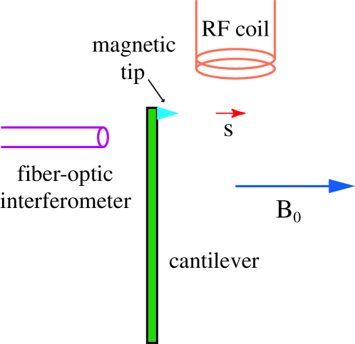
Figure 1: Schematic diagram of the MRFM setup.

A schematic illustration of the MRFM setup is shown in Fig 1. A uniform magnetic field, $B_{0}$, points in the positive $z$-direction. A single spin is placed in front of the cantilever tip which can oscillate only in the $z$-direction. A ferromagnetic particle (or small magnetic material) mounted on the cantilever tip produces a non-uniform magnetic field or magnetic field gradient of $({\partial B_{z}}/{\partial Z})_{0}$ on the single spin. As a result, a reactive force (or interaction) acts back on the magnetic cantilever tip in the $z$-direction from the single spin. The origin is chosen to be the equilibrium position of the cantilever tip without the presence of the spin.

In CAI, the cantilever is driven at its resonance frequency to amplify the otherwise very small vibrational amplitude. This is achieved by a modulation scheme using the frequency modulation of a rotating radio-frequency (RF) magnetic field in the $x$-$y$ plane. In this case, the rotating RF field can be represented as $B_{1x}=B_{1}\cos\{[\omega+\Delta\omega(t)]t\}$, $B_{1y}=-B_{1}\sin\{[\omega+\Delta\omega(t)]t\}$, where the frequency modulation $\Delta\omega(t)$ is a periodic function in time with the resonant frequency $\omega_{m}$ of the cantilever. In the reference frame rotating with the ${\mathbf{B}}_{1}$, the spin-cantilever Hamiltonian can be written as

$${\hat{H}}_{SZ}(t)={\hat{H}}_{Z}-\hbar\left[\omega_{L}-\omega-\Delta\omega(t)\right]{\hat{S}}_{z}-\hbar\omega_{1}{\hat{S}}_{x}-g\mu\left({{\partial B_{z}}\over{\partial Z}}\right)_{0}{\hat{Z}}{\hat{S}}_{z}\;,$$ (1)

where $\omega_{L}=g\mu B_{z}/\hbar$ and $\omega_{1}=g\mu B_{1}/\hbar$ are respectively the Larmor and Rabi frequencies, $B_{z}$ includes the uniform magnetic field $B_{0}$ and the magnetic field produced by the ferromagnetic particle, $g$ and $\mu$ are the $g$-factor and the electron or nuclear magneton, and

$${\hat{H}}_{Z}=\frac{1}{2m}{\hat{p}}^{2}+\frac{m\omega_{m}^{2}}{2}{\hat{Z}}^{2}$$ (2)

is the Hamiltonian of the cantilever in isolation (i.e., with no external magnetic field coupling it to the spin). For $\omega=\omega_{L}$, we arrive at an effective cantilever-spin Hamiltonian of the form

$${\hat{H}}_{SZ}(t)={\hat{H}}_{Z}-2\eta{\hat{Z}}{\hat{S}}_{z}+f(t){\hat{S}}_{z}-\varepsilon{\hat{S}}_{x}\;,$$ (3)

where $f(t)=\Delta\omega(t)$, $\eta=(g\mu/2)({\partial B_{z}}/{\partial Z})_{0}$ and $\varepsilon=\hbar\omega_{1}$. We will discuss in details the rotating picture and adiabatic approximation for the spin-cantilever system in the next section.

In the following, we briefly describe the basic principle of the single-spin measurement by CAI MRFM. In the case when the adiabatic approximation is exact, the instantaneous eigenstates of the spin Hamiltonian in the rotating frame of the ${\mathbf{B}}_{1}$ field are the spin states parallel or antiparallel to the direction of the effective magnetic field ${\mathbf{B}}^{\rm eff}(t)=\left(\varepsilon,0,-f(t)\right)$, denoted as $|v_{\pm}(t)\rangle$, respectively. We define an operator ${\hat{S}}_{z}^{\prime}$ for the component of spin along this axis. Note that the initial spin state in the laboratory frame has the same expression as the initial state in the rotating frame. Starting at a general initial spin state (in the laboratory or rotating frame) of

$$\chi(0)=a|\uparrow\rangle+b|\downarrow\rangle$$ (4)

in the ${\hat{S}}_{z}$ representation, we can rewrite this initial state in the basis of the instantaneous eigenstates of ${\hat{S}}_{z}^{\prime}$ as

$$\chi(0)=a_{\rm eff}|v_{+}(0)\rangle+b_{\rm eff}|v_{-}(0)\rangle,$$ (5)

where

$$a_{\rm eff} = a\cos(\Theta_{0}/2)+b\sin(\Theta_{0}/2),$$ (6)

$$b_{\rm eff} = -a\sin(\Theta_{0}/2)+b\cos(\Theta_{0}/2),$$ (7)

and $\Theta_{0}\equiv\Theta(0)$ is the initial angle between the effective magnetic magnetic field and the $z$-axis direction. This implies $\tan[\Theta(t)]=B_{x}^{\rm eff}(t)/B_{z}^{\rm eff}(t)=-\varepsilon/f(t)$. It then follows from the adiabatic theorem that the spin state at time $t$ can be written as:

$$\chi(t) = a_{\rm eff}|v_{+}(t)\rangle\,\exp({-\frac{i}{\hbar}\int_{0}^{t}\lambda_{+}(t^{\prime})dt^{\prime}})$$ (8)

$$+b_{\rm eff}|v_{-}(t)\rangle\,\exp({-\frac{i}{\hbar}\int_{0}^{t}\lambda_{-}(t^{\prime})dt^{\prime}}),$$

where $\lambda_{\pm}(t)$ are instantaneous eigenvalues. So the probabilities of finding the spin to be in the instantaneous eigenstates $|v_{\pm}(t)\rangle$ are respectively $|a_{\rm eff}|^{2}$ and $|b_{\rm eff}|^{2}$. Since the coefficients $a_{\rm eff}$ and $b_{\rm eff}$ are time independent, the probabilities $|a_{\rm eff}|^{2}$ and $|b_{\rm eff}|^{2}$ remain the same at all times. This provides us with an opportunity to measure the initial spin state probabilities at later times.

How do we measure these spin state probabilities? The idea is to transfer the information of the spin state to the state of the driven cantilever. In the interaction picture in which the state is rotating with the instantaneous eigenstates of the spin Hamiltonian, the spin-cantilever interaction can be written as $2\eta{\hat{Z}}{\hat{S}}_{z}^{\prime}\cos[\Theta(t)]$. As a result, the phase of the driven cantilever vibrations depends on the orientation of the spin states. Suppose that the initial state is a product state of the cantilever and spin parts. At a later time, due to the interaction between them, the total state becomes entangled. Monitoring the phase of the cantilever vibrations will give us the information about the spin. Numerical simulations (see Fig. 4 with reasonable parameters for the CAI approximations) indicate that as the amplitude of the cantilever vibrations increases with time, the phase difference in the oscillations for the two different initial spin eigenstates of ${\hat{S}}_{z}^{\prime}$ approaches $\pi$. In other words, the measurement of the single-spin states can be achieved by monitoring the phases of the cantilever vibrations at some later time $t$. Phase-sensitive, optical homodyne measurements of the cantilever vibrations can be performed using a fiber-optic interferometer. The main purpose of this paper is to present a realistic and detailed analysis of the single-spin measurement scheme, including the effects of the measurement device and other relevant sources of noise.

3 The rotating picture and adiabatic approximation

We assume an effective cantilever-spin Hamiltonian of the form (3) where for the moment we let $f(t)$ and $\varepsilon$ be arbitrary, and ${\hat{H}}_{Z}$ is the Hamiltonian given by (2). It is useful to group this into three terms

$${\hat{H}}_{SZ}(t)={\hat{H}}_{Z}+{\hat{H}}_{I}+{\hat{H}}_{S}(t)\;,$$ (9)

where

$${\hat{H}}_{I} \equiv -2\eta{\hat{Z}}{\hat{S}}_{z}\;,$$

$${\hat{H}}_{S}(t) \equiv f(t){\hat{S}}_{z}-\varepsilon{\hat{S}}_{x}\;.$$ (10)

The state of the cantilever-spin system evolves according to the Schrödinger equation

$$\frac{d{|\psi(t)\rangle}}{dt}=-\frac{i}{\hbar}{\hat{H}}_{SZ}(t){|\psi(t)\rangle}\;.$$ (11)

In realistic cases, the spin part of the Hamiltonian (representing precession under the magnetic field) gives an evolution which is very rapid compared to the reaction time of the cantilever. It therefore makes sense to switch to an interaction picture in which the state is rotating along with this precession. We do this by introducing a (partial) time translation operator

$${\hat{U}}_{S}(t)\equiv:\exp-\frac{i}{\hbar}\left[\int_{0}^{t}{\hat{H}}_{S}(t^{\prime})dt^{\prime}\right]:\;,$$ (12)

where $::$ indicates that the integral is to be taken in a time-ordered sense; this unitary operator obeys the differential equation

$$\frac{d{\hat{U}}_{S}(t)}{dt}=-\frac{i}{\hbar}{\hat{H}}_{S}(t){\hat{U}}_{S}(t)\;.$$ (13)

We then introduce the state ${|\tilde{\psi}(t)\rangle}$ in the rotating picture:

$${|\tilde{\psi}(t)\rangle}\equiv{\hat{U}}^{\dagger}_{S}(t){|\psi(t)\rangle}\;,$$ (14)

with ${|\psi(t)\rangle}$ the solution of the original Schrödinger equation (11) at time $t$. The evolution equation for ${|\tilde{\psi}(t)\rangle}$ is

$$\frac{d{|\tilde{\psi}(t)\rangle}}{dt} = \frac{d{\hat{U}}^{\dagger}_{S}(t)}{dt}{|\psi(t)\rangle}+{\hat{U}}^{\dagger}_{S}(t)\frac{d{|\psi(t)\rangle}}{dt}$$ (15)

$$= \frac{i}{\hbar}{\hat{U}}^{\dagger}_{S}(t){\hat{H}}_{S}(t){|\psi(t)\rangle}-\frac{i}{\hbar}{\hat{U}}^{\dagger}_{S}(t){\hat{H}}_{SZ}(t){|\psi(t)\rangle}$$

$$= -\frac{i}{\hbar}{\hat{H}}_{Z}{|\tilde{\psi}(t)\rangle}-\frac{i}{\hbar}\left[{\hat{U}}^{\dagger}_{S}(t){\hat{H}}_{I}{\hat{U}}_{S}(t)\right]{|\tilde{\psi}(t)\rangle}$$

$$= -\frac{i}{\hbar}{\hat{H}}_{Z}{|\tilde{\psi}(t)\rangle}+\frac{2i\eta}{\hbar}{\hat{Z}}\left[{\hat{U}}^{\dagger}_{S}(t){\hat{S}}_{z}{\hat{U}}_{S}(t)\right]{|\tilde{\psi}(t)\rangle}\;.$$

We can define a locked spin operator ${\hat{S}}_{L}(t)$

$${\hat{S}}_{L}(t)\equiv\left[{\hat{U}}^{\dagger}_{S}(t){\hat{S}}_{z}{\hat{U}}_{S}(t)\right]\;;$$ (16)

in terms of this, the equation of motion for ${|\tilde{\psi}\rangle}$ becomes

$$\frac{d{|\tilde{\psi}(t)\rangle}}{dt}=-\frac{i}{\hbar}{\hat{H}}_{Z}{|\tilde{\psi}(t)\rangle}+\frac{2i\eta}{\hbar}{\hat{Z}}{\hat{S}}_{L}(t){|\tilde{\psi}(t)\rangle}\;.$$ (17)

Unfortunately, it is difficult to get an exact solution for ${\hat{U}}_{S}(t)$ for a general function $f(t)$. This means that it is also difficult to derive an exact expression for ${\hat{S}}_{L}(t)$, and the rotating picture (15), while formally correct, is not very helpful.

However, while we cannot easily find an exact expression for ${\hat{U}}_{S}(t)$ for general $f(t)$, we can easily find an approximate solution for a large class of functions. Suppose that $\varepsilon$ is large and $f(t)$ is slowly varying, so that $|f(t)|,\varepsilon\gg|f^{\prime}(t)/f(t)|$ for typical values of $f(t)$ and $f^{\prime}(t)$. Then ${\hat{H}}_{S}(t)$ is also slowly varying, and if a spin begins in an instantaneous eigenstate of ${\hat{H}}_{S}(t)$, it will remain close to an instantaneous eigenstate of ${\hat{H}}_{S}(t)$ for all times by the adiabatic theorem.

The instantaneous eigenstates of ${\hat{H}}_{S}(t)$ are

$${\hat{H}}_{S}(t){|v_{\pm}(t)\rangle}=\lambda_{\pm}(t){|v_{\pm}(t)\rangle}\equiv\pm\lambda(t){|v_{\pm}(t)\rangle}\;,$$ (18)

where

$$\lambda(t) = \sqrt{f^{2}(t)+\varepsilon^{2}}\;,$$

$${|v_{\pm}(t)\rangle} = \frac{\varepsilon}{\sqrt{(f(t)\mp\lambda(t))^{2}+\varepsilon^{2}}}{|\downarrow\rangle}-\frac{f(t)\mp\lambda(t)}{\sqrt{(f(t)\mp\lambda(t))^{2}+\varepsilon^{2}}}{|\uparrow\rangle}\;.$$ (19)

We use these instantaneous eigenvectors and eigenvalues to define an approximation to the unitary operator ${\hat{U}}_{S}(t)$:

$${\hat{U}}^{\prime}_{S}(t)={\hat{I}}\otimes{|v_{+}(t)\rangle}{\langle v_{+}(0)|}{\rm e}^{-i\Phi(t)}+{\hat{I}}\otimes{|v_{-}(t)\rangle}{\langle v_{-}(0)|}{\rm e}^{i\Phi(t)}\;,$$ (20)

with the accumulated phase

$$\Phi(t)\equiv\frac{1}{\hbar}\int_{0}^{t}\lambda(t^{\prime})dt^{\prime}\;.$$ (21)

Note that $\Phi(t)$ obeys $d\Phi(t)/dt=\lambda(t)$. This implies that

$$\frac{d{\hat{U}}^{\prime}_{S}(t)}{dt} = -\frac{i}{\hbar}\lambda(t){\hat{I}}\otimes{|v_{+}(t)\rangle}{\langle v_{+}(0)|}{\rm e}^{-i\Phi(t)}+\frac{i}{\hbar}\lambda(t){\hat{I}}\otimes{|v_{-}(t)\rangle}{\langle v_{-}(0)|}{\rm e}^{i\Phi(t)}$$ (22)

$$+{\hat{I}}\otimes\frac{d{|v_{+}(t)\rangle}}{dt}{\langle v_{+}(0)|}{\rm e}^{-i\Phi(t)}+{\hat{I}}\otimes\frac{d{|v_{-}(t)\rangle}}{dt}{\langle v_{-}(0)|}{\rm e}^{i\Phi(t)}$$

$$= -\frac{i}{\hbar}{\hat{H}}_{S}(t){\hat{U}}^{\prime}_{S}(t)+{\hat{I}}\otimes\frac{d{|v_{+}(t)\rangle}}{dt}{\langle v_{+}(0)|}{\rm e}^{-i\Phi(t)}$$

$$+{\hat{I}}\otimes\frac{d{|v_{-}(t)\rangle}}{dt}{\langle v_{-}(0)|}{\rm e}^{i\Phi(t)}\;,$$

which has the form of (13) plus some additional terms. From the definition (19) of ${|v_{\pm}(t)\rangle}$, we see

$$\frac{d{|v_{\pm}(t)\rangle}}{dt}=\pm\frac{1}{2}\frac{\varepsilon}{\lambda^{2}(t)}\frac{df(t)}{dt}{|v_{\mp}(t)\rangle}\;.$$ (23)

Provided that $f(t)$ is slowly varying, the additional terms in (22) will be small.

Just as before, we can define a rotating picture, now using the unitary transformation ${\hat{U}}^{\prime}_{S}(t)$,

$${|\breve{\psi}(t)\rangle}\equiv\left({\hat{U}}^{\prime}_{S}(t)\right)^{\dagger}{|\psi(t)\rangle}\;.$$ (24)

This gives us a new evolution equation for ${|\breve{\psi}\rangle}$:

$$\frac{d{|\breve{\psi}(t)\rangle}}{dt} = \frac{d({\hat{U}}^{\prime}_{S}(t))^{\dagger}}{dt}{|\psi(t)\rangle}+({\hat{U}}^{\prime}_{S}(t))^{\dagger}\frac{d{|\psi(t)\rangle}}{dt}$$ (25)

$$= -\frac{i}{\hbar}{\hat{H}}_{Z}{|\breve{\psi}(t)\rangle}+\frac{2i\eta}{\hbar}{\hat{Z}}\left[({\hat{U}}^{\prime}_{S}(t))^{\dagger}{\hat{S}}_{z}{\hat{U}}^{\prime}_{S}(t)\right]{|\breve{\psi}(t)\rangle}$$

$$+{\hat{I}}\otimes\Biggl{(}{|v_{+}(0)\rangle}\frac{d{\langle v_{+}(t)|}}{dt}{\rm e}^{-i\Phi(t)}$$

$$+{|v_{-}(0)\rangle}\frac{d{\langle v_{-}(t)|}}{dt}{\rm e}^{i\Phi(t)}\Biggr{)}{\hat{U}}^{\prime}_{S}(t){|\breve{\psi}(t)\rangle}\;.$$

At this point, it is helpful to introduce a new set of spin operators

$${\hat{S}}_{x}^{\prime} = \frac{\hbar}{2}{\hat{I}}\otimes\left({|v_{+}(0)\rangle}{\langle v_{-}(0)|}+{|v_{-}(0)\rangle}{\langle v_{+}(0)|}\right)\;,$$

$${\hat{S}}_{y}^{\prime} = \frac{i\hbar}{2}{\hat{I}}\otimes\left({|v_{-}(0)\rangle}{\langle v_{+}(0)|}-{|v_{+}(0)\rangle}{\langle v_{-}(0)|}\right)\;,$$

$${\hat{S}}_{z}^{\prime} = \frac{\hbar}{2}{\hat{I}}\otimes\left({|v_{+}(0)\rangle}{\langle v_{+}(0)|}-{|v_{-}(0)\rangle}{\langle v_{-}(0)|}\right)\;.$$ (26)

Using the definition (20) for ${\hat{U}}^{\prime}_{S}(t)$, we can solve for the various terms in (25):

$$({\hat{U}}^{\prime}_{S}(t))^{\dagger}{\hat{S}}_{z}{\hat{U}}^{\prime}_{S}(t)=-\frac{f(t)}{\lambda(t)}{\hat{S}}_{z}^{\prime}-\frac{\varepsilon}{\lambda(t)}\left({\hat{S}}_{x}^{\prime}\cos(2\Phi(t))-{\hat{S}}_{y}^{\prime}\sin(2\Phi(t))\right)\;.$$ (27)

$${\hat{I}}\otimes\left({|v_{+}(0)\rangle}\frac{d{\langle v_{+}(t)|}}{dt}{\rm e}^{-i\Phi(t)}+{|v_{-}(0)\rangle}\frac{d{\langle v_{-}(t)|}}{dt}{\rm e}^{i\Phi(t)}\right){\hat{U}}^{\prime}_{S}(t)=\ \ \$$

$$\frac{i\varepsilon}{\hbar\lambda^{2}(t)}\frac{df(t)}{dt}\left({\hat{S}}_{x}^{\prime}\sin(2\Phi(t))+{\hat{S}}_{y}^{\prime}\cos(2\Phi(t))\right)\;.$$ (28)

Substituting (26–28) into (25), we get

$$\frac{d{|\breve{\psi}(t)\rangle}}{dt} = -\frac{i}{\hbar}{\hat{H}}_{Z}{|\breve{\psi}(t)\rangle}+\frac{2i\eta}{\hbar}{\hat{Z}}\frac{f(t)}{\lambda(t)}{\hat{S}}_{z}^{\prime}{|\breve{\psi}(t)\rangle}$$ (29)

$$+\frac{2i\eta}{\hbar}{\hat{Z}}\frac{\varepsilon}{\lambda(t)}\left({\hat{S}}_{x}^{\prime}\cos(2\Phi(t))-{\hat{S}}_{y}^{\prime}\sin(2\Phi(t))\right){|\breve{\psi}(t)\rangle}$$

$$+i\frac{\varepsilon}{\hbar\lambda^{2}(t)}\frac{df(t)}{dt}\left({\hat{S}}_{x}^{\prime}\sin(2\Phi(t))+{\hat{S}}_{y}^{\prime}\cos(2\Phi(t))\right){|\breve{\psi}(t)\rangle}\;.$$

Note that this equation is still exact—it is equivalent to the original Schrödinger equation (11). However, we can see that if $|f(t)|,\varepsilon$ are large, then $\Phi(t)$ will be a rapidly growing function, and the last two terms of equation (29) will oscillate very rapidly compared to the first two terms. Over a short period relative to the response time of the cantilever they will essentially average away to nothing. In this limit, therefore, we can reasonably make a rotating-wave approximation, to get the approximate evolution equation

$$\frac{d{|\breve{\psi}(t)\rangle}}{dt}\approx-\frac{i}{\hbar}\left({\hat{H}}_{Z}-2\eta(f(t)/\lambda(t)){\hat{Z}}{\hat{S}}_{z}^{\prime}\right){|\breve{\psi}(t)\rangle}\;.$$ (30)

This is equivalent to making an exact adiabatic approximation, as described in section 2. We can see how this approximation compares to the complete Hamiltonian for a reasonable set of parameter values in figures 2 and 3. This set of parameters was chosen to match those of Berman et al. [9], as was the set of times plotted in figure 3. Comparison shows that our results match their unitary simulations to good precision. For the rest of this paper we will be using the rotating wave approximation, and representing states in the rotating frame. For simplicity, we henceforth omit the accent from the state ${|\breve{\psi}\rangle}$.

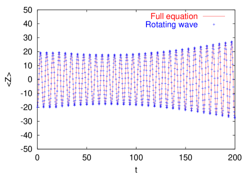
Figure 2: Mean cantilever position ${\langle{\hat{Z}}\rangle}$ vs. $t$ for the complete and rotating wave Hamiltonians.

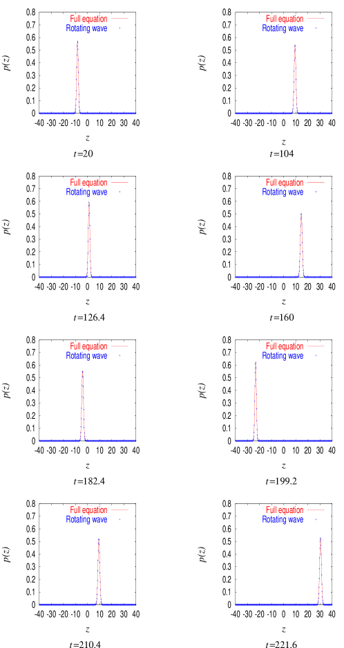
Figure 3: The probability distribution, $p(z)$, of finding the cantilever at position $z$ at a range of times for the complete and rotating wave Hamiltonians.

In this rotating-wave approximation, if the spin begins in an instantaneous eigenstate of ${\hat{H}}_{S}(t)$, it will remain in an instantaneous eigenstate at all times. If it begins in a superposition of the two eigenstates, the spin and cantilever degrees of freedom will become entangled, with the two components of the wavefunction corresponding to the two spin directions remaining undisturbed for all times. Monitoring the position of the cantilever then serves as a nondemolition measurement of the spin, as we would wish.

Note that the corrections to the adiabatic approximation include terms which can flip the spin. These terms must remain small for the system to be a true nondemolition measurement. The result of the spin measurement manifests itself as a $\pi$ phase shift in the oscillation of the cantilever. We can see this in figure 4.

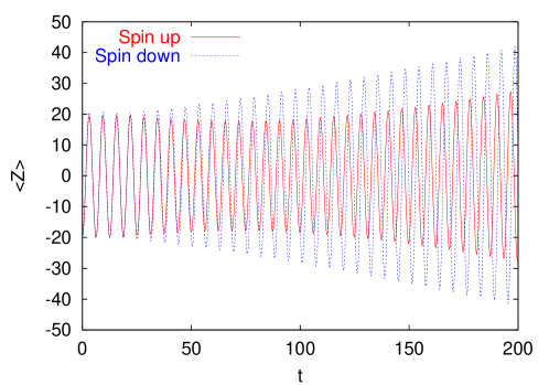
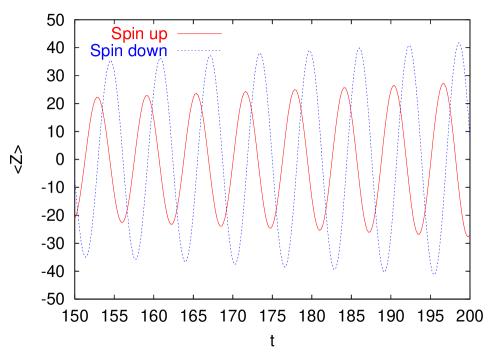
Figure 4: Mean cantilever position ${\langle{\hat{Z}}\rangle}$ vs. $t$ for initial spin up and down in the ${\hat{S}}_{z}^{\prime}$ direction.

4 The thermal environment

Unfortunately, in practice we cannot treat the cantilever as an isolated system. It is coupled at least weakly to the vibrational modes of the bulk, and is therefore subject to dissipation and thermal noise. Since the cantilever can be treated as a single harmonic oscillator, we can model the effects of this thermal bath by the well-known Caldeira-Leggett [14] master equation in the high-temperature limit:

$${\dot{\rho}}=-\frac{i}{\hbar}[{\hat{H}}_{SZ}(t),\rho]-\frac{i\gamma_{m}}{\hbar}[{\hat{Z}},\{{\hat{p}},\rho\}]-\frac{\gamma_{m}}{2\ell^{2}}[{\hat{Z}},[{\hat{Z}},\rho]]\;,$$ (31)

where the parameters are

$$\gamma_{m} = \frac{\Gamma}{2m}\;,$$

$$\ell = \frac{\hbar}{2\sqrt{mkT}}\;,$$ (32)

$m$ is the cantilever mass, $T$ is the temperature, $k$ is Boltzmann’s constant (or the equivalent for our system of units), and $\Gamma$ is the strength of the coupling to the thermal bath. We can interpret $\gamma_{m}$ (with units of inverse time) as the dissipation rate and $\ell$ (with units of length) as the thermal de Broglie wavelength.

A feature of this equation is that it doesn’t necessarily preserve the positivity of $\rho$ on short time scales (though at long times it is well-behaved) [17]. This arises because of the approximations which are made in the derivation, which become invalid at very short times. While this may be physically unimportant, it can be inconvenient; in particular, if we wish to unravel the evolution into a stochastic Schrödinger equation [23] (as we will in section 6), it is necessary to start with a master equation in Lindblad form, [16]

$${\dot{\rho}}=-\frac{i}{\hbar}[{\hat{H}},\rho]+\sum_{j}\left[2{\hat{L}}_{j}\rho{\hat{L}}^{\dagger}_{j}-\{{\hat{L}}^{\dagger}_{j}{\hat{L}}_{j},\rho\}\right]\;,$$ (33)

for some Hermitian ${\hat{H}}$ and set of general Lindblad operators $\{{\hat{L}}_{j}\}$. The Caldeira-Leggett equation (31) is not of this form, which is why it can violate positivity of $\rho$.

The exact quantum Brownian motion master equation was shown [17] not to have the Lindblad form, but rather requires time-dependent coefficients to ensure the positivity of the density matrix at short times. However, by keeping more terms from the high- or medium-temperature-limit expansion in a consistent way, Diósi [18] has shown that the Caldeira-Leggett equation can be replaced by another master equation which is of Lindblad form, and which agrees with it except at very short times when the equation’s validity is questionable in any case. This is done by adding a term to (31) of the form $-(\gamma_{m}\ell^{2}/2\hbar^{2})[{\hat{p}},[{\hat{p}},\rho]]$. The procedure is analogous to completing the square. If we choose the ansatz

$${\hat{L}}=A{\hat{Z}}+iB{\hat{p}}$$ (34)

with real $A,B$, plug it into the equation (33), and equate it to the Caldeira-Leggett equation (31) plus the additional term, we get

$${\dot{\rho}} = -(i/\hbar)[{\hat{H}},\rho]-A^{2}[{\hat{Z}},[{\hat{Z}},\rho]]-B^{2}[{\hat{p}},[{\hat{p}},\rho]]$$ (35)

$$+iAB(-2{\hat{Z}}\rho{\hat{p}}+{\hat{Z}}{\hat{p}}\rho+\rho{\hat{Z}}{\hat{p}}+2{\hat{p}}\rho{\hat{Z}}-{\hat{p}}{\hat{Z}}\rho-\rho{\hat{p}}{\hat{Z}})$$

$$= -(i/\hbar)[{\hat{H}}_{SZ}(t),\rho]-\frac{\gamma_{m}}{2\ell^{2}}[{\hat{Z}},[{\hat{Z}},\rho]]-\frac{\gamma_{m}\ell^{2}}{2\hbar^{2}}[{\hat{p}},[{\hat{p}},\rho]]$$

$$+\frac{i\gamma_{m}}{\hbar}({\hat{p}}\rho{\hat{Z}}-{\hat{Z}}{\hat{p}}\rho-{\hat{Z}}\rho{\hat{p}}+\rho{\hat{p}}{\hat{Z}})\;,$$

which implies that

$$A = \sqrt{\gamma_{m}/2\ell^{2}}\;,$$

$$B = \sqrt{\gamma_{m}\ell^{2}/2\hbar^{2}}\;,$$

$${\hat{H}} = {\hat{H}}_{SZ}(t)+(\gamma_{m}/2)({\hat{Z}}{\hat{p}}+{\hat{p}}{\hat{Z}})\equiv{\hat{H}}^{\prime}_{SZ}(t)\;.$$ (36)

So the Lindblad operator for this equation is

$${\hat{L}}=\sqrt{\gamma_{m}/2}\left((1/\ell){\hat{Z}}+i(\ell/\hbar){\hat{p}}\right)\;,$$ (37)

and the effective Hamiltonian, going to the rotating picture and making use of the approximation derived in section 3, is

$${\hat{H}}^{\prime}_{SZ}(t)=\frac{1}{2m}{\hat{p}}^{2}+\frac{m\omega_{m}^{2}}{2}{\hat{Z}}^{2}-2\eta(f(t)/\lambda(t)){\hat{Z}}{\hat{S}}_{z}^{\prime}+(\gamma_{m}/2)({\hat{Z}}{\hat{p}}+{\hat{p}}{\hat{Z}})\;.$$ (38)

In order for the cantilever to be an effective measurement device, the loss rate must be very low: $\omega_{m}\gg\gamma_{m}$.

5 The effects of monitoring

In order to serve as a measurement scheme, we must have some way of monitoring the motion of the cantilever. Because of the microscopic scale of the motion, this is not so easily done. One approach is to use optical interferometry to measure the cantilever position.

As shown in figure 1, the cantilever forms one side of an optical microcavity and the cleaved end of the fiber forms the other side. As the cantilever moves, the resonant frequency of the cavity changes. Because the timescale of the cantilever’s motion is very long compared to the optical timescale, we can treat the effects of this in the adiabatic limit. The cavity mode is also subject to driving by an external laser, and has a very high loss rate. The full master equation [19] for the cantilever-spin-cavity system in the interaction picture is

$${\dot{\rho}} = -\frac{i}{\hbar}[{\hat{H}}^{\prime}_{SZ}(t),\rho]+2{\hat{L}}\rho{\hat{L}}^{\dagger}-{\hat{L}}^{\dagger}{\hat{L}}\rho-\rho{\hat{L}}^{\dagger}{\hat{L}}$$ (39)

$$-i[E({\hat{a}}^{\dagger}+{\hat{a}})+{\hat{a}}^{\dagger}{\hat{a}}(\Delta+\kappa{\hat{Z}}),\rho]$$

$$+(\gamma_{c}/2)(2{\hat{a}}\rho{\hat{a}}^{\dagger}-{\hat{a}}^{\dagger}{\hat{a}}\rho-\rho{\hat{a}}^{\dagger}{\hat{a}})\;,$$

where ${\hat{H}}^{\prime}_{SZ}(t)$ and ${\hat{L}}$ are the Hamiltonian and Lindblad operator for the cantilever and spin given by eqns. (37) and (38), $E$ is the strength of the laser driving, $\Delta$ is the detuning from the “neutral” cavity frequency, $\kappa$ is the coupling strength of the cantilever to the cavity mode, and $\gamma_{c}$ is the loss rate of the cavity.

Suppose now that we perform homodyne measurement [15, 20] on the light which escapes from the cavity. We would like to replace the equation (39) above with an equation for the conditional evolution of $\rho$, conditioned on the output photocurrent $I_{c}(t)$. The conditional evolution equation for our system then becomes [20, 21] (in Itô calculus form)

$$d\rho = -\frac{i}{\hbar}[{\hat{H}}^{\prime}_{SZ}(t),\rho]dt+\left(2{\hat{L}}\rho{\hat{L}}^{\dagger}-{\hat{L}}^{\dagger}{\hat{L}}\rho-\rho{\hat{L}}^{\dagger}{\hat{L}}\right)dt$$ (40)

$$-i[E({\hat{a}}^{\dagger}+{\hat{a}})+{\hat{a}}^{\dagger}{\hat{a}}(\Delta+\kappa{\hat{Z}}),\rho]dt$$

$$+(\gamma_{c}/2)\left(2{\hat{a}}\rho{\hat{a}}^{\dagger}-{\hat{a}}^{\dagger}{\hat{a}}\rho-\rho{\hat{a}}^{\dagger}{\hat{a}}\right)dt$$

$$+\sqrt{\gamma_{c}e_{d}}\left({\hat{a}}\rho+\rho{\hat{a}}^{\dagger}-{\langle{\hat{a}}+{\hat{a}}^{\dagger}\rangle}\rho\right)dW_{t}\;,$$

where $0\leq e_{d}\leq 1$ is the detector efficiency and $dW_{t}$ is a real stochastic differential variable which obeys the statistics

$$M[dW_{t}]=0\;,\ \ M[dW_{t}dW_{s}]=\delta(t-s)dt\;.$$ (41)

This noise is related to the output photocurrent [15, 20, 21]

$$I_{c}(t)=\beta\left[\gamma_{c}e_{d}{\langle{\hat{a}}+{\hat{a}}^{\dagger}\rangle}_{t}+\sqrt{\gamma_{c}e_{d}}\frac{dW_{t}}{dt}\right]\;,$$ (42)

where $\beta$ is a constant giving the device’s range of response.

We want to operate in the “bad cavity” limit where $\gamma_{c}\gg\omega_{m}$. This means that the cavity mode will approach equilibrium on a timescale very short compared to that of the cantilever’s motion, so that the cavity mode can be adiabatically eliminated [19, 20, 21] from this equation, leaving an equation in terms of the spin and cantilever position alone.

Let the detuning vanish $\Delta\rightarrow 0$ and the coupling $\kappa$ to the cantilever be very small. If we initially neglect this coupling altogether, we can solve for the steady-state of the cavity mode in isolation from the cantilever:

$$-i[E({\hat{a}}^{\dagger}+{\hat{a}}),\rho]+(\gamma_{c}/2)\left(2{\hat{a}}\rho{\hat{a}}^{\dagger}-{\hat{a}}^{\dagger}{\hat{a}}\rho-\rho{\hat{a}}^{\dagger}{\hat{a}}\right) = 0\;,$$

$$\left({\hat{a}}\rho+\rho{\hat{a}}^{\dagger}-{\langle{\hat{a}}+{\hat{a}}^{\dagger}\rangle}\rho\right) = 0\;,$$ (43)

which implies that $\rho={|\alpha_{0}\rangle}{\langle\alpha_{0}|}$, where ${\hat{a}}{|\alpha_{0}\rangle}=\alpha_{0}{|\alpha_{0}\rangle}$ is a coherent state with

$$\alpha_{0}=-\frac{2iE}{\gamma_{c}}\;.$$ (44)

Now let us restore the coupling $\kappa$ between the cantilever and the cavity mode. If this coupling is very small, then the state of the cavity mode will remain very close to the state ${|\alpha_{0}\rangle}$. In this case, it is very useful to switch to a displaced basis [19, 20, 21] for the cavity mode. We switch from the operators ${\hat{a}},{\hat{a}}^{\dagger}$ to displaced operators

$${\hat{b}}\equiv{\hat{a}}-\alpha_{0}\;,$$

$${\hat{b}}^{\dagger}\equiv{\hat{a}}^{\dagger}-\alpha^{*}_{0}\;,$$ (45)

and displaced number states

$${\hat{b}}^{\dagger}{\hat{b}}{|n\rangle}=n{|n\rangle}\;.$$ (46)

Obviously ${|0\rangle}={|\alpha_{0}\rangle}$, and ${|1\rangle}={\hat{a}}^{\dagger}{|\alpha_{0}\rangle}-\alpha_{0}^{*}{|\alpha_{0}\rangle}$.

We now make the ansatz of keeping the two lowest displaced number states ${|0,1\rangle}$ of the cavity mode and neglecting the rest. [20, 19, 21] We then write the full density matrix for the spin-cantilever-cavity system as

$$\rho(t)=\rho_{0}(t)\otimes{|0\rangle}{\langle 0|}+\rho_{1}(t)\otimes{|1\rangle}{\langle 0|}+\rho_{1}^{\dagger}(t)\otimes{|0\rangle}{\langle 1|}+\rho_{2}(t)\otimes{|1\rangle}{\langle 1|}\;,$$ (47)

where $\rho_{0,1,2}$ are operators which act on the Hilbert space of the cantilever and spin, and $\rho_{0,2}$ are self-adjoint. The reduced density matrix of the spin-cantilever alone is obtained by tracing out the cavity mode, yielding

$$\rho_{SZ}(t)=\rho_{0}(t)+\rho_{2}(t)\;.$$ (48)

If we substitute the definitions (45) and (47) into the stochastic master equation (40) and collect terms, we get a set of coupled equations in the operators $\rho_{0,1,2}$:

$$d\rho_{0} = \left(-\frac{i}{\hbar}[{\hat{H}}^{\prime}_{SZ}(t),\rho_{0}]+2{\hat{L}}\rho_{0}{\hat{L}}^{\dagger}-{\hat{L}}^{\dagger}{\hat{L}}\rho_{0}-\rho_{0}{\hat{L}}^{\dagger}{\hat{L}}\right)dt$$ (49)

$$-\frac{4i\kappa E^{2}}{\gamma_{c}^{2}}[{\hat{Z}},\rho_{0}]dt+\frac{2\kappa E}{\gamma_{c}}({\hat{Z}}\rho_{1}+\rho_{1}^{\dagger}{\hat{Z}})dt+\gamma_{c}\rho_{2}dt$$

$$+\sqrt{\gamma_{c}e_{d}}\left(\rho_{1}+\rho_{1}^{\dagger}-\rho_{0}{\rm Tr}\{\rho_{1}+\rho_{1}^{\dagger}\}\right)dW_{t}\;,$$

$$d\rho_{1} = \left(-\frac{i}{\hbar}[{\hat{H}}^{\prime}_{SZ}(t),\rho_{1}]+2{\hat{L}}\rho_{1}{\hat{L}}^{\dagger}-{\hat{L}}^{\dagger}{\hat{L}}\rho_{1}-\rho_{1}{\hat{L}}^{\dagger}{\hat{L}}\right)dt$$ (50)

$$-i\kappa{\hat{Z}}\rho_{1}dt-\frac{4i\kappa E^{2}}{\gamma_{c}^{2}}[{\hat{Z}},\rho_{1}]dt-\frac{2\kappa E}{\gamma_{c}}({\hat{Z}}\rho_{0}-\rho_{2}{\hat{Z}})dt-(\gamma_{c}/2)\rho_{1}dt$$

$$+\sqrt{\gamma_{c}e_{d}}\left(\rho_{2}-\rho_{1}{\rm Tr}\{\rho_{1}+\rho_{1}^{\dagger}\}\right)dW_{t}\;,$$

$$d\rho_{2} = \left(-\frac{i}{\hbar}[{\hat{H}}^{\prime}_{SZ}(t),\rho_{2}]+2{\hat{L}}\rho_{2}{\hat{L}}^{\dagger}-{\hat{L}}^{\dagger}{\hat{L}}\rho_{2}-\rho_{2}{\hat{L}}^{\dagger}{\hat{L}}\right)dt$$ (51)

$$-\left(i\kappa+\frac{4i\kappa E^{2}}{\gamma_{c}^{2}}\right)[{\hat{Z}},\rho_{2}]dt-\frac{2\kappa E}{\gamma_{c}}({\hat{Z}}\rho_{1}^{\dagger}+\rho_{1}{\hat{Z}})dt-\gamma_{c}\rho_{2}dt$$

$$-\sqrt{\gamma_{c}e_{d}}\rho_{2}{\rm Tr}\{\rho_{1}+\rho_{1}^{\dagger}\}dW_{t}\;.$$

Both $\rho_{1}$ and $\rho_{2}$ contain damping terms, which imply that they will remain small at all times provided $\kappa{\hat{Z}}$ is sufficiently small compared to $\gamma_{c}$. (This also implies that our ansatz is reasonable for sufficiently small $\kappa$.)

By making use of the above equations, we can find the evolution equation for the reduced density matrix $\rho_{SZ}$:

$$d\rho_{SZ}(t) = d\rho_{0}(t)+d\rho_{2}(t)$$ (52)

$$= \left(-\frac{i}{\hbar}[{\hat{H}}^{\prime}_{SZ}(t),\rho_{SZ}]+2{\hat{L}}\rho_{SZ}{\hat{L}}^{\dagger}-{\hat{L}}^{\dagger}{\hat{L}}\rho_{SZ}-\rho_{SZ}{\hat{L}}^{\dagger}{\hat{L}}\right)dt$$

$$-\frac{4i\kappa E^{2}}{\gamma_{c}^{2}}[{\hat{Z}},\rho_{SZ}]dt+\frac{2\kappa E}{\gamma_{c}}[{\hat{Z}},\rho_{1}-\rho_{1}^{\dagger}]dt-i\kappa[{\hat{Z}},\rho_{2}]dt$$

$$+\sqrt{\gamma_{c}e_{d}}\left(\rho_{1}+\rho_{1}^{\dagger}-\rho_{SZ}{\rm Tr}\{\rho_{1}+\rho_{1}^{\dagger}\}\right)dW_{t}\;.$$

If we keep only terms to second order in $\kappa{\hat{Z}}$ we can neglect the $\rho_{2}$ term. This leaves only the terms proportional to $\rho_{1}\pm\rho_{1}^{\dagger}$, which we need only know to leading order in $\kappa{\hat{Z}}$. Provided (as we have already assumed) that the cantilever moves slowly compared to the timescale set by $\gamma_{c}$ and that $\kappa{\hat{Z}}$ can be treated as small, then to leading order $d\rho_{1}$ vanishes; $\rho_{1}$ remains in an approximate equilibrium state. If we make use of this assumption we can (again to leading order) solve for $\rho_{1}\pm\rho_{1}^{\dagger}$:

$$\rho_{1}+\rho_{1}^{\dagger} \approx -\frac{4\kappa E}{\gamma_{c}^{2}}\{{\hat{Z}},\rho_{SZ}\}\;,$$

$$\rho_{1}-\rho_{1}^{\dagger} \approx -\frac{4\kappa E}{\gamma_{c}^{2}}[{\hat{Z}},\rho_{SZ}]\;,$$ (53)

which when inserted into (52) gives us a closed evolution equation for $\rho_{SZ}$:

$$d\rho_{SZ}(t) = \left(-\frac{i}{\hbar}[{\hat{H}}^{\prime}_{SZ}(t),\rho_{SZ}]+2{\hat{L}}\rho_{SZ}{\hat{L}}^{\dagger}-{\hat{L}}^{\dagger}{\hat{L}}\rho_{SZ}-\rho_{SZ}{\hat{L}}^{\dagger}{\hat{L}}\right)dt$$ (54)

$$-\frac{4i\kappa E^{2}}{\gamma_{c}^{2}}[{\hat{Z}},\rho_{SZ}]dt-\frac{8\kappa^{2}E^{2}}{\gamma_{c}^{3}}[{\hat{Z}},[{\hat{Z}},\rho_{SZ}]]dt$$

$$+\sqrt{\gamma_{c}e_{d}}\frac{4\kappa E}{\gamma_{c}^{2}}\left({\hat{Z}}\rho_{SZ}+\rho_{SZ}{\hat{Z}}-2\rho_{SZ}{\rm Tr}\{\rho_{SZ}\}\right)dW_{t}\;.$$

(Note that we have absorbed a factor of $-1$ into $dW_{t}$.)

Examining the terms in (54), we see that by eliminating the cavity mode we get another effective term in the Hamiltonian, and another Lindblad operator. We can therefore write this stochastic master equation in the form

$$d\rho_{SZ}(t) = -\frac{i}{\hbar}[{\hat{H}}_{\rm eff}(t),\rho_{SZ}]dt+\sum_{j=1}^{2}\left(2{\hat{L}}_{j}\rho_{SZ}{\hat{L}}^{\dagger}_{j}-{\hat{L}}^{\dagger}_{j}{\hat{L}}_{j}\rho_{SZ}-\rho_{SZ}{\hat{L}}^{\dagger}_{j}{\hat{L}}_{j}\right)dt$$ (55)

$$+\sqrt{e_{d}/2}\left(({\hat{L}}_{2}-{\langle{\hat{L}}_{2}\rangle})\rho_{SZ}+\rho_{SZ}({\hat{L}}_{2}-{\langle{\hat{L}}_{2}\rangle})\right)dW_{t}\;,$$

where we now make the definitions

$${\hat{L}}_{1} = \sqrt{\gamma_{m}/2}\left((1/\ell){\hat{Z}}+i(\ell/\hbar){\hat{p}}\right)$$

$${\hat{L}}_{2} = \sqrt{8\kappa^{2}E^{2}/\gamma_{c}^{3}}{\hat{Z}}\;,$$

$${\hat{H}}_{\rm eff}(t) = \frac{1}{2m}{\hat{p}}^{2}+\frac{m\omega_{m}^{2}}{2}{\hat{Z}}^{2}-2\eta(f(t)/\lambda(t)){\hat{Z}}{\hat{S}}_{z}^{\prime}$$ (56)

$$+\frac{4\kappa E^{2}}{\gamma_{c}^{2}}{\hat{Z}}+(\gamma_{m}/2)({\hat{Z}}{\hat{p}}+{\hat{p}}{\hat{Z}})\;.$$

Note that the term $4\kappa E^{2}{\hat{Z}}/\gamma_{c}^{2}$ is a constant force, which just displaces the equilibrium position of the cantilever. It can be eliminated simply by changing the origin of ${\hat{Z}}$, and is in any case small for reasonable values of the parameters. The output from the homodyne measurement now corresponds to a measurement of the cantilever position ${\langle{\hat{Z}}\rangle}$:

$$I_{c}(t)=\beta\left(-\frac{8e_{d}\kappa E}{\gamma_{c}}{\langle{\hat{Z}}\rangle}+\sqrt{\gamma_{c}e_{d}}\frac{dW_{t}}{dt}\right)\;.$$ (57)

As we shall see in the next section, we can further unravel this stochastic master equation (55) into a stochastic Schrödinger equation for pure states. This further unraveling provides considerable improvement in numerical efficiency, though it does not represent an actual measurement process.

6 Pure state unraveling

The stochastic master equation (55) represents the evolution of the cantilever-spin system, conditioned on the photocurrent measurement record $I_{c}(t)$. If we averaged over all possible measurement records, the $dW_{t}$ terms would average to zero, and we would be left with an ordinary deterministic master equation for the cantilever and spin. It is for this reason that the stochastic master equation is therefore often referred to as an unraveling of the average master equation.

For numerical purposes, it is often much easier to solve an equation for a pure state vector rather than a density matrix [22, 23]. It is therefore useful to unravel equation (55) still further to an equation which preserves pure states. We do this by introducing a second stochastic process.

First, let us idealize to perfect detector efficiency $e_{d}=1$. We then introduce the new master equation

$$d\rho_{SZ}(t) = -\frac{i}{\hbar}[{\hat{H}}_{\rm eff}(t),\rho_{SZ}]dt+\sum_{j=1}^{2}\left(2{\hat{L}}_{j}\rho_{SZ}{\hat{L}}^{\dagger}_{j}-{\hat{L}}^{\dagger}_{j}{\hat{L}}_{j}\rho_{SZ}-\rho_{SZ}{\hat{L}}^{\dagger}_{j}{\hat{L}}_{j}\right)dt$$ (58)

$$+\sum_{j=1}^{2}\left(({\hat{L}}_{j}-{\langle{\hat{L}}_{j}\rangle})\rho_{SZ}+\rho_{SZ}({\hat{L}}_{j}-{\langle{\hat{L}}_{j}\rangle})\right)dW_{jt}\;,$$

where the Hamiltonian and Lindblad operators are the same as in (56) and we now have two independent noise processes represented by stochastic differential variables $dW_{1t}$ and $dW_{2t}$ which satisfy

$$M[dW_{jt}]=0\;,\ \ dW_{it}dW_{js}=\delta(t-s)\delta_{ij}dt\;.$$ (59)

If we take the mean of (58) over $dW_{1t}$ we recover equation (55). We can think of the additional stochastic process as representing a fictitious additional measurement, whose outcome we average over to recover the state which is conditioned on the actual measurement.

However, equation (58) has a great advantage over (55). If $\rho_{SZ}$ is initially a pure state $\rho_{SZ}={|\psi_{SZ}\rangle}{\langle\psi_{SZ}|}$, it will remain a pure state at all times, the state of course depending on the stochastic processes $W_{1}$ and $W_{2}$. We can recover the solution of (55) by averaging

$$\rho_{SZ}(t)=M_{W_{1}}[{|\psi_{SZ}(t)\rangle}{\langle\psi_{SZ}(t)|}]\;.$$ (60)

It would be useful to replace equation (58) with an explicit evolution equation for ${|\psi_{SZ}\rangle}$ instead of $\rho_{SZ}$. This equation is the quantum state diffusion equation with real noise [24, 25]:

$$d{|\psi_{SZ}\rangle} = -\frac{i}{\hbar}{\hat{H}}_{\rm eff}(t){|\psi_{SZ}\rangle}dt+\frac{1}{\sqrt{2}}\sum_{j}\left(2{\langle{\hat{L}}^{\dagger}_{j}\rangle}{\hat{L}}_{j}-{\hat{L}}^{\dagger}_{j}{\hat{L}}_{j}-|{\langle{\hat{L}}_{j}\rangle}|^{2}\right){|\psi_{SZ}\rangle}dt$$ (61)

$$+\frac{1}{\sqrt{2}}\sum_{j}\left({\hat{L}}_{j}-{\langle{\hat{L}}_{j}\rangle}\right){|\psi_{SZ}\rangle}dW_{jt}\;.$$

The nonlinearity of this equation arises to preserve the norm.

7 Numerical simulation

We have simulated this system using the C++ quantum state diffusion library [26] to numerically solve both the unitary evolution with Hamiltonian (30) and the stochastic equation (61). All of the figures in this paper were generated using this software.

We chose our parameters based on those used by Berman et al., [9]. These values are (in arbitrary units):

$$\hbar = \omega_{m}=m=1\;,$$

$$\eta = 0.3\;,$$

$$\varepsilon = 400.0\;,$$

$$\gamma_{m} = \omega_{m}/Q=0.00001\;,$$

$$k_{B}T = 10000.0\;,$$ (62)

where $Q$ is the quality factor of the cantilever. The driving force $f(t)$ takes the form

$$f(t)=\cases{-6000+300t&if $0\leq t\leq 20$;\cr 1000\sin(t-20)&if $t>20$.}$$ (63)

If we make contact with physical values for actual cantilevers used in experiments, we have $\omega_{m}\approx 10^{5}{\rm s}^{-1}$ and $m\approx 10^{-12}{\rm kg}$. The value of $k_{B}T$ above then corresponds to a temperature of around $0.1{\rm K}$, which is within the bounds of experimental feasibility, though rather lower than the temperatures used in current experiments (around 3K) [11]. Since $\eta=(g\mu/2)(\partial B_{z}/\partial Z)_{0}$, the value of $\eta$ corresponds to a field gradient of about $1.5\times 10^{7}{\rm T/m}$, which is higher than current experiments by roughly two orders of magnitude [11], but hopefully this too will improve with time. The cantilever would undergo displacements of about a nanometer.

Alternatively, rather than increasing the field gradient we could achieve similar numbers by lowering the spring constant of the cantilever, for instance by shrinking the mass of the cantilever. Lowering the mass by a factor of 100 has the same relative effect on $\eta$ as increasing the field gradient by a factor of ten.

We then might ask about realistic parameters for the monitoring. A typical cavity size $L$ is about a micrometer, with a laser frequency of $\omega_{c}\approx 1.4\times 10^{15}{\rm s}^{-1}$. This cavity is generally quite lossy; reasonable quality factors might be in the range $Q_{c}\sim$10–100. The parameter $E$ is a function of the laser power, $E=\sqrt{P\gamma_{c}/\hbar\omega_{c}}=\sqrt{P/\hbar Q_{c}}$. For $P\sim 1\mu{\rm W}$ and $Q_{c}\sim 100$ we have $E\sim 10^{13}{\rm s}^{-1}$. The coupling between the cantilever and the cavity is given by a geometric factor $\kappa=\omega_{c}/L\sim 1.4\times 10^{21}({\rm m}\cdot{\rm s})^{-1}$. In arbitrary units, this gives coefficients

$$\frac{8\kappa E}{\gamma_{c}} = 1.9\times 10^{3}\;,$$

$$\frac{4\kappa E^{2}}{\gamma_{c}^{2}} = 7\times 10^{2}\;,$$

$$\sqrt{\frac{8\kappa^{2}E^{2}}{\gamma_{c}^{3}}} = 0.07\;.$$ (64)

The first value is the multiplier in (57); the second gives the equilibrium displacement of the cantilever; the third is the coefficient of the Lindblad operator ${\hat{L}}_{2}$.

One question we can now easily address is how quickly the state of the spin collapses onto eigenstates of ${\hat{S}}_{z}^{\prime}$. In figure 5 we plot ${\langle{\hat{S}}_{z}^{\prime}\rangle}$ for ten different trajectories. We see that in all ten cases the spin converged to $\pm 1/2$ quite quickly, before $t=80$.

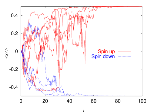
Figure 5: Expectation value ${\langle{\hat{S}}_{z}^{\prime}\rangle}$ vs. t in arbitrary units for ten different trajectories, showing the rapid localization of the spin, for an initial superposition state $\left(|v_{+}(0)\rangle+|v_{-}(0)\rangle\right)/\sqrt{2}$.

If we compare this to the results of figure 4, we see that the spin state collapses rather more quickly than the cantilever oscillations can respond. We only get a clear output signal when the two phases are well separated, which does not occur until nearly $t=150$. Generically, the difficulty of collapsing the spin state is much less than the difficulty of obtaining an unequivocal readout.

The curves depicted in figure 4 are idealized, without the measurement noise which will always be present in the output current (42) or (57). In figure 6 we show what actual output would look like for the set of parameters we are discussing. Note that even with the noise, the two phases (representing spin up and spin down) are clearly distinguishable. In the next section, we derive an expression for the signal-to-noise ratio in more general situations.

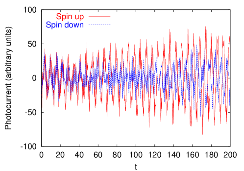
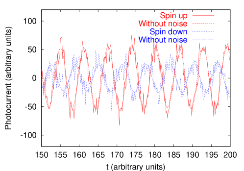
Figure 6: Simulation of photocurrent output in arbitrary units, including measurement noise, using parameters of section 7. We have chosen the scale $\beta$ so that the vertical scale matches that of figure 4, and also plotted the signals without the noisy $dW/dt$ components.

8 Signal-to-noise ratio

Since we have to detect the effect of very weak force on the cantilever by the single spin, we need very high resolution for the cantilever position measurements and a good control of the various noise sources in the MRFM device. As described in section 2, the tiny displacement of the cantilever is measured by a fiber-optic interferometer as a phase shift of the interference fringes. We shall analyze the quantum and thermal noise in this homodyne measurement scheme.

The Hamiltonian for the combined system of the spin, cantilever and cavity mode, excluding coupling to the environments, in the spin rotating frame is

$$\hat{H} = \hat{H}_{Z}-2\eta\frac{f(t)}{\lambda(t)}{\hat{Z}}{\hat{S}}_{z}^{\prime}+\hbar\omega_{c}{\hat{a}}^{\dagger}{\hat{a}}$$ (65)

$$+\hbar E({\hat{a}}^{\dagger}e^{-i\omega_{0}t}+{\hat{a}}e^{i\omega_{0}t})+\hbar\kappa{\hat{a}}^{\dagger}{\hat{a}}\hat{Z}.$$

Here $\omega_{c}$ is the optical frequency of the cavity mode, $\omega_{0}\sim\omega_{c}$ is the driving frequency of the external laser and other terms and parameters have been described in section 5. The master equation approach in section 4 is valid in high or medium temperature case. Here we analyze the noise in the Heisenberg picture, using the quantum Langevin equation approach that is valid at any temperature. [27]

Using standard techniques, [28, 29] the reservoir (environmental) variables may be eliminated, in the interaction picture with respect to $\hbar\omega_{0}{\hat{a}}^{\dagger}{\hat{a}}$, to give the quantum Langevin equations describing the dynamics of the whole system:

$$\frac{d{\hat{Z}}(t)}{dt} = \frac{1}{m}{\hat{p}}(t),$$ (66)

$$\frac{d{\hat{p}}(t)}{dt} = -m\omega_{m}^{2}{\hat{Z}}(t)-\frac{\Gamma}{m}{\hat{p}}(t)-\hbar\kappa{\hat{a}}^{\dagger}(t){\hat{a}}(t)+\hat{{\cal W}}(t)+2\eta\frac{f(t)}{\lambda(t)}{\hat{S}}_{z}^{\prime}(t),$$ (67)

$$\frac{d{\hat{a}}(t)}{dt} = -(i\omega_{c}-i\omega_{0}+\frac{\gamma_{c}}{2}){\hat{a}}(t)-i\kappa{\hat{Z}}(t){\hat{a}}(t)-iE+\sqrt{\gamma_{c}}{\hat{a}}_{\rm in}(t),$$ (68)

$$\frac{d{\hat{S}}_{z}^{\prime}(t)}{dt} = 0,$$ (69)

$$\frac{d{\hat{S}}_{x}^{\prime}(t)}{dt} = 2\eta\frac{f(t)}{\lambda(t)}{\hat{Z}}(t){\hat{S}}_{y}^{\prime}(t),$$ (70)

$$\frac{d{\hat{S}}_{y}^{\prime}(t)}{dt} = -2\eta\frac{f(t)}{\lambda(t)}{\hat{Z}}(t){\hat{S}}_{x}^{\prime}(t).$$ (71)

In the equations, the usual optical input noise operator ${\hat{a}}_{\rm in}(t)$ is associated with the vacuum fluctuations of the continuum of electromagnetic modes outside the cavity and its correlation function is given by

$$\langle{\hat{a}}_{\rm in}(t){\hat{a}}^{\dagger}_{\rm in}(t^{\prime})\rangle=\delta(t-t^{\prime}).$$ (72)

The random force $\hat{\cal W}(t)$ describes the thermal noise motion (quantum Brownian motion) of the cantilever at temperature $T$. For the case of an Ohmic environment, the thermal random force correlation is given by [27]

$$\langle\hat{\cal W}(t)\hat{\cal W}(t^{\prime})\rangle=\frac{\hbar\Gamma}{\pi}[{\cal F}_{r}(t-t^{\prime})+i{\cal F}_{i}(t-t^{\prime})],$$ (73)

where

$${\cal F}_{r}(t) = \int_{0}^{\Omega}d\omega\,\omega\cos(\omega t)\coth\left(\frac{\hbar\omega}{2k_{B}T}\right),$$ (74)

$${\cal F}_{i}(t) = \int_{0}^{\Omega}d\omega\,\omega\sin(\omega t),$$ (75)

with $\Omega$ the frequency cutoff of the reservoir spectrum. Without the presence of the external driving force from the spin, the cantilever-cavity system can be characterized by a semi-classical steady state with a new equilibrium position for the cantilever, displaced by $Z_{st}=-\kappa|\alpha_{st}|^{2}/(m\omega_{m}^{2})$ with respect to that with no external driving laser field, and the cavity mode in a coherent state $|\alpha_{st}\rangle$ with the amplitude given by

$$\alpha_{st}=\frac{-iE}{\gamma_{c}/2+i\Delta},$$ (76)

where $\Delta=\omega_{c}-\omega_{0}-\kappa^{2}|\alpha_{st}|^{2}/(m\omega_{m}^{2})$ is the cavity mode detuning. By adjusting either $\omega_{0}$ or $\omega_{c}$, the detuning can be set to zero $\Delta=0$. As a result, $\alpha_{st}=\alpha_{0}=-2iE/\gamma_{c}$. Linearizing the quantum Langevin equations about the steady-state values and renaming with ${\hat{Z}}(t)$, ${\hat{a}}(t)$ the operators describing the quantum fluctuations around the classical steady state, we obtain

$$\frac{d{\hat{Z}}(t)}{dt} = \frac{1}{m}{\hat{p}}(t),$$ (77)

$$\frac{d{\hat{p}}(t)}{dt} = -m\omega_{m}^{2}{\hat{Z}}(t)-\frac{\Gamma}{m}{\hat{p}}(t)-\hbar\kappa[\alpha_{0}{\hat{a}}^{\dagger}(t)+\alpha_{0}^{*}{\hat{a}}(t)]$$ (78)

$$+\hat{{\cal W}}(t)+2\eta\frac{f(t)}{\lambda(t)}{\hat{S}}_{z}^{\prime}(t),$$

$$\frac{d{\hat{a}}(t)}{dt} = -\frac{\gamma_{c}}{2}{\hat{a}}(t)-i\kappa\alpha_{0}{\hat{Z}}(t)+\sqrt{\gamma_{c}}{\hat{a}}_{\rm in}(t),$$ (79)

$$\frac{d{\hat{S}}_{z}^{\prime}(t)}{dt} = 0,$$ (80)

$$\frac{d{\hat{S}}_{x}^{\prime}(t)}{dt} = 2\eta\frac{f(t)}{\lambda(t)}[Z_{st}+{\hat{Z}}(t)]{\hat{S}}_{y}^{\prime}(t),$$ (81)

$$\frac{d{\hat{S}}_{y}^{\prime}(t)}{dt} = -2\eta\frac{f(t)}{\lambda(t)}[Z_{st}+{\hat{Z}}(t)]{\hat{S}}_{x}^{\prime}(t).$$ (82)

In the bad cavity limit where $\gamma_{c}\gg\omega_{m},(\Gamma/m),\kappa{\hat{Z}}$ [i.e., set $(d{\hat{a}}(t)/dt)=0$ in (79)], the dynamics of the field quadrature, ${\hat{a}}^{\dagger}(t)+{\hat{a}}(t)$, adiabatically follows that of the cantilever position:

$${\hat{a}}^{\dagger}(t)+{\hat{a}}(t)=-i\frac{4\kappa\alpha_{0}}{\gamma_{c}}{\hat{Z}}(t)+\frac{2}{\sqrt{\gamma_{c}}}[{\hat{a}}_{\rm in}(t)+{\hat{a}}^{\dagger}_{\rm in}(t)].$$ (83)

Thus monitoring this field quadrature of the cavity mode via homodyne measurement corresponds to a measurement of the cantilever position and hence the state of the spin. Using the usual input-output relation, [28, 29]

$${\hat{a}}_{\rm out}(t)=\sqrt{\gamma_{c}}{\hat{a}}(t)-{\hat{a}}_{\rm in},$$ (84)

we may define an operator corresponding to the output current

$$\hat{I}_{\rm out}(t) = \sqrt{\gamma_{c}}\beta[{\hat{a}}_{\rm out}(t)+{\hat{a}}^{\dagger}_{\rm out}(t)]$$ (85)

$$= \beta\{\gamma_{c}[{\hat{a}}(t)+{\hat{a}}^{\dagger}(t)]-\sqrt{\gamma_{c}}[{\hat{a}}_{\rm in}(t)+{\hat{a}}^{\dagger}_{\rm in}(t)]\}.$$

Equation (85) is similar to (42) with $e_{d}=1$. By substituting (83) into (85), the resultant output current in the bad cavity limit is given by

$$\hat{I}_{\rm out}(t)=\beta\left(\frac{-8\kappa E}{\gamma_{c}}{\hat{Z}}(t)+\sqrt{\gamma_{c}}\,[{\hat{a}}_{\rm in}(t)+{\hat{a}}^{\dagger}_{\rm in}(t)]\right)\;.$$ (86)

This equation is also similar to (57) with $e_{d}=1$, obtained from master equation approach.

The Langevin equations for ${\hat{S}}_{x}^{\prime}$ and ${\hat{S}}_{y}^{\prime}$ effectively decouple from the other equations, since they do not appear on the right-hand-side of the equations for the other variables. Because of this, they have no effect in our estimate of the signal-to-noise ratio, and we shall drop them henceforth. Taking a Fourier transform of the linearized Langevin equations, we find, from (85), the Fourier component of the output current as

$$\hat{I}_{\rm out}(\omega) = -\frac{\beta\gamma_{c}}{(i\omega-\gamma_{c}/2)}\Biggl{\{}\left(i\omega+\frac{\gamma_{c}}{2}\right)[{\hat{a}}_{\rm in}(\omega)+{\hat{a}}^{\dagger}_{\rm in}(\omega)]$$ (87)

$$-\frac{2i\kappa\alpha_{0}\sqrt{\gamma_{c}}}{m(\omega_{m}^{2}-\omega^{2}-i\Gamma\omega/m)}\Biggl{[}\frac{\hbar\kappa\alpha_{0}\sqrt{\gamma_{c}}}{(i\omega-\gamma_{c}/2)}[{\hat{a}}^{\dagger}_{\rm in}(\omega)-{\hat{a}}_{\rm in}(\omega)]$$

$$\qquad\qquad\qquad+\hat{\cal W}(\omega)+G(\omega){\hat{S}}_{z}^{\prime}]\Biggr{]}\Biggr{\}},$$

where $G(\omega)$ is the Fourier transform of $G(t)=2\eta{f(t)}/{\lambda(t)}$. The Fourier component of the mean output current signal is then given by

$$|\langle\hat{I}_{\rm out}(\omega)\rangle|=\beta\gamma_{c}\left(\frac{2\kappa\sqrt{\gamma_{c}}|\alpha_{0}|}{m}\right)\frac{|G(\omega)|}{|D(\omega)|}\langle{\hat{S}}_{z}^{\prime}\rangle,$$ (88)

where

$$D(\omega)=\left(i\omega-\frac{\gamma_{c}}{2}\right)\left(\omega_{m}^{2}-\omega^{2}-i\omega\frac{\Gamma}{m}\right).$$ (89)

The output current noise power density spectrum is defined as

$$S_{\rm out}(\omega) = \left\{\int d\tau\,e^{i\omega\tau}\langle\hat{I}_{\rm out}(t)\hat{I}_{\rm out}(t+\tau)\rangle_{G(t)=0}\right\}_{t}$$ (90)

$$= \frac{1}{2\pi}\left\{\int d\omega^{\prime}e^{-i(\omega+\omega^{\prime})t}\langle\hat{I}_{\rm out}(\omega^{\prime})I_{\rm out}(\omega)\rangle_{G(\omega)=0}\right\}_{t},$$

where the subscript $G(t)=0$ means evaluation in the absence of the external driving force from the spin and $\{\cdots\}_{t}$ denotes the time average over $t$. To calculate this noise spectrum, the Fourier transform of the noise correlation functions (72)–(75) is needed and given by

$$\langle{\hat{a}}_{\rm in}(\omega){\hat{a}}^{\dagger}_{\rm in}(\omega^{\prime})\rangle = 2\pi\delta(\omega+\omega^{\prime}),$$ (91)

$$\langle\hat{\cal W}(\omega)\hat{\cal W}(\omega^{\prime})\rangle = 2\pi\hbar\Gamma\omega\left[1+\coth\left(\frac{\hbar\omega}{2k_{B}T}\right)\right]\delta(\omega+\omega^{\prime}),$$ (92)

where in obtaining (92) the infinite frequency cutoff limit of the Ohmic thermal reservoir spectrum, $\Omega\to\infty$, has been assumed. After some calculations, one can then obtain the output noise spectrum as

$$S_{\rm out}(\omega) = \beta^{2}\gamma_{c}^{2}\left\{1+4\left(\frac{\hbar\kappa^{2}\gamma_{c}|\alpha_{0}|^{2}}{m}\right)^{2}\frac{1}{[(\gamma_{c}/2)^{2}+\omega^{2}]|D(\omega)|^{2}}\right.$$ (93)

$$\left.\quad+4\left(\frac{\kappa^{2}\gamma_{c}|\alpha_{0}|^{2}\Gamma}{m^{2}}\right)\frac{\hbar\omega}{|D(\omega)|^{2}}\coth\left(\frac{\hbar\omega}{2k_{B}T}\right)\right\}.$$

The first term in (93), independent of frequency, is the contribution from the shot noise of the photons. The next term is the “back-action” noise on the position of the cantilever by the radiation (photons). This back action is due to the random way in which photons bounce off the cantilever. The final term is the thermal noise, due to the thermal Brownian-motion fluctuation of the cantilever. Equation (93) is valid at all temperatures. The assumptions made in its derivation are the linearization around the semi-classical steady state and the infinite frequency cutoff $\Omega\to\infty$. The high (or medium) temperature limit $\hbar\omega_{m}\ll k_{B}T$ can be obtained by approximating

$$\hbar\omega\coth\left(\frac{\hbar\omega}{2k_{B}T}\right)\approx 2k_{B}T+\frac{\hbar^{2}\omega^{2}}{6k_{B}T}.$$ (94)

We plot these three contributions to the noise for the simulation parameters given in section 7. We see that at the oscillator resonance $\omega_{m}=1$, thermal noise dominates.

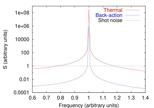
Figure 7: We plot the various terms of $S_{\rm out}(\omega)$ vs. $\omega$, using the parameters of section 7. We have scaled $\gamma_{c}\beta=1$. Note that at $\omega=\omega_{m}=1$ the thermal noise dominates.

Let us define the signal-to-noise ratio per root Hertz as

$${\rm SNR}(\omega)=\frac{|\langle\hat{I}_{\rm out}(\omega)\rangle|}{\sqrt{S_{\rm out}(\omega)}}.$$ (95)

We are interested in evaluating SNR$(\omega)$ at the frequency equal to the cantilever vibration frequency, $\omega=\omega_{m}$. Note that

$$\frac{1}{|D(\omega_{m})|}=\frac{1}{[(\gamma_{c}/2)^{2}+\omega_{m}^{2}]^{1/2}}\left(\frac{Q}{\omega_{m}^{2}}\right),$$ (96)

where the quality factor $Q={m\omega_{m}}/{\Gamma}$. As a result, the mean output current signal (88) at $\omega=\omega_{m}$ is enhanced by a factor of $Q\gamma_{c}/[(\gamma_{c}/2)^{2}+\omega_{m}^{2}]^{1/2}$ as compared with the $\omega=0$ case. However, a similar enhancement occurs in the back-action noise and the thermal noise terms. In other words, driving the cantilever at $\omega=\omega_{m}$ amplifies not only its vibration amplitudes due to the the driving force, but also the noise amplitude due to the back-action radiation pressure and thermal Brownian motion (see Fig. 7). We find ${\rm SNR}(\omega=\omega_{m})$ can be written as

$${\rm SNR}(\omega_{m})=\frac{|G(\omega_{m})|\langle{\hat{S}}_{z}^{\prime}\rangle}{\sqrt{N(\omega_{m})}}$$ (97)

where

$$N(\omega_{m})=\frac{[(\gamma_{c}/2)^{2}+\omega_{m}^{2}]}{4\kappa^{2}\gamma_{c}|\alpha_{0}|^{2}}\left(\frac{m\omega_{m}^{2}}{Q}\right)^{2}+\frac{\hbar^{2}\kappa^{2}\gamma_{c}|\alpha_{0}|^{2}}{[(\gamma_{c}/2)^{2}+\omega_{m}^{2}]}+\Gamma\hbar\omega_{m}\coth\left(\frac{\hbar\omega_{m}}{2k_{B}T}\right).$$ (98)

We may set $\langle{\hat{S}}_{z}^{\prime}\rangle=\pm(1/2)$ to estimate the signal-to-noise ratio per root Hz, corresponding respectively to the spin in the two different states in the rotating frame.

Because the driving force $f(t)$ is periodic, $G(\omega)$ is equal to a sum of delta functions at $\omega=\omega_{m},3\omega_{m},5\omega_{m},\ldots$. Averaging over a small interval about $\omega_{m}$, we can integrate over the delta function to get a value (for our simulation parameters) of ${\rm SNR}(\omega_{m})\approx 220{\rm s}^{-1/2}$. Thus, given a bandwidth of about 1Hz, this should be easily detectable by our measurement scheme. As mentioned in section 7, we have assumed a magnetic field gradient roughly two orders of magnitude greater than current experiments, and a much lower temperature. A single spin, therefore, would be below the edge of detectability by current experimental techniques. Steady improvement in the field strength, temperature and spring constant of these experiments, however, should soon make single-spin measurement possible.

If the dominant noise source in MRFM comes from the thermal Brownian motion of the cantilever, we can estimate the minimum detectable force (when the signal-to-noise ratio is one) by keeping only the last term of (98). In this case, with a measurement bandwith $\Delta\nu$, we obtain from (97), (98) and (94) the usual expression of the minimum detectable force at the high-temperature limit ($\hbar\omega_{m}\ll k_{B}T$) as

$$F_{\min}=\sqrt{N(\omega_{m})\Delta\nu}=\sqrt{\frac{2kk_{B}T\Delta\nu}{Q\omega_{m}}}\;,$$ (99)

where $k=m\omega_{m}^{2}$ is the spring constant of the cantilever. We see, then, that improvement can come either from raising the force (by increasing the field gradient), lowering the temperature, or lowering the spring constant.

9 Conclusion

We have derived an approximate description of single-spin measurement by magnetic resonance force microscopy, including both thermal noise and measurement back-action, and used it to produce numerical simulations of a single-spin measurement. These simulations use the quantum trajectory method for open quantum systems. The parameters we assumed for this simulation were somewhat optimistic; but given the steady improvement in experimental technique, we believe that measurements of this type will be possible in the near future.

Single-spin measurements would be very useful in the construction of solid-state quantum computers, in which the spin of an electron represents a single qubit of information. Given the great interest in solid-state implementations as a possibly scalable realization of quantum computers, finding practical ways to measure single spins would be very useful. The results of our simulations suggest that magnetic resonance force microscopy is a very promising approach to this difficult problem.

References

[1]
D. Loss and D. P. DiVincenzo,
Phys. Rev. A 57, 120 (1998).
[2]
B.E. Kane, Nature
393, 133-137 (1998).
[3]
R. Vrijen, E. Yablonovitch, K. Wang, H. W. Jiang, A. Balandin,
V. Roychowdhury, T. Mor, and D. DiVincenzo
Phys. Rev. A 62, 012306 (2000).
[4]
G.P. Berman, G.D. Doolen, P.C. Hammel, and V.I. Tsifrinovich,
Phys. Rev. B 61, 14694 (2000).
[5]
J. Twamley, quant-ph/0210202.
[6]
H.-A. Engel and D. Loss
Phys. Rev. B 65, 195321 (2002).
[7]
J.A. Sidles,
Appl. Phys. Lett. 58, 2854 (1991).
[8]
J.A. Sidles,
Phys. Rev. Lett. 68, 1124 (1992).
[9]
G.P Berman, F. Borgonovi, G. Chapline, S.A. Gurvitz, P.C. Hammel,
D.V. Pelekhov, A. Suter and V.I. Tsifrinovich, quant-ph/0108025.
[10]
K. Wago, D. Botkin, C.S. Yannoni, and D. Rugar,
Phys. Rev. B 57, 1108 (1998).
[11]
B. C. Stipe, H. J. Mamin, C. S. Yannoni,
T. D. Stowe, T. W. Kenny, and D. Rugar,
Phys. Rev. Lett. 87, 277602 (2001).
[12]
D. Rugar, O. Züger, S. Hoen, C.S. Yannoni, H.M. Vieth, and R.D. Kendrick,
Science 264, 1560 (1994).
[13]
G.P. Berman, F. Borgonovi, H.-S. Goan, S.A. Gurvitz and
V.I. Tsifrinovich, quant-ph/0210043, to appear in Phys. Rev. B.
[14]
A.O. Caldeira and A.J. Leggett, Physica A 121, 587 (1983).
[15] H. J. Carmichael, An Open System Approach
to Quantum Optics, Lecture notes in physics (Springer-Verlag,
Berlin, 1993).
[16] G. Lindblad, Commun. Math. Phys.
48, 199 (1976).
[17] B.-L. Hu, J.P. Paz and Y. Zhang,
Phys. Rev. D 45, 2843 (1992).
[18]L. Diósi, Europhys. Lett. 22, 1 (1993);
Physica A 199, 517 (1993).
[19] G. J. Milburn, K. Jacobs and D. F. Walls
Phys. Rev. A 50, 5256 (1994).
[20] H. M. Wiseman and G.J. Milburn,
Phys. Rev. A 47, 642 (1993); 47, 1652 (1993).
[21] A. C. Doherty and K. Jacobs,
Phys. Rev. A 60, 2700 (1999).
[22] R. Schack, T. A. Brun, I. C. Percival,
J. Phys. A. 28, 5401 (1995).
[23] See, for example, H. J. Carmichael (guest Ed), Quantum
Semiclass. Opt. 8, 47-314 (1996) special issue and
references therein.
[24] N. Gisin, Phys. Rev. Lett. 52, 1657 (1984).
[25] N. Gisin and I. C. Percival, J. Phys. A 25,
5677 (1992); ibid.26, 2245 (1993).
[26]
R. Schack and T. A. Brun, Comp. Phys. Comm. 102, 210 (1997).
[27]
V. Giovannetti and D. Vitali, Phys. Rev. A 63, 023812 (2001).
[28] D. F. Walls and G. J. Milburn, Quantum Optics,
(Springer-Verlag, Berlin, 1994).
[29] C. W. Gardiner and P. Zoller, Quantum Noise,
2nd ed. (Springer-Verlag, Berlin, 2000).