A Magnetic Resonance Realization of Decoherence-Free Quantum Computation

Abstract

We report the realization, using nuclear magnetic resonance techniques, of the first quantum computer that reliably executes an algorithm in the presence of strong decoherence. The computer is based on a quantum error avoidance code that protects against a class of multiple-qubit errors. The code stores two decoherence-free logical qubits in four noisy physical qubits. The computer successfully executes Grover’s search algorithm in the presence of arbitrarily strong engineered decoherence. A control computer with no decoherence protection consistently fails under the same conditions.

A computer that uses the laws of quantum mechanics to store and manipulate information could in theory perform certain tasks such as searching Grover (1997) and factoring Shor (1997) with incredible efficiency. The most critical problem that must be solved to make quantum computing possible on a useful scale is decoherence, the inevitable process of entanglement between a quantum computer and its environment. Decoherence causes the superposition states that carry information within the computer to decay rapidly. Several solutions to the decoherence problem have been proposed (for a review, see Nielsen and Chuang (2000)). One technique, quantum error avoidance, calls for information within the computer to be carried exclusively by quantum states that are not adversely affected by decoherence Zanardi and Rasetti (1998); Duan and Guo (1998); Lidar et al. (1998, 2001a) (for a review, see Lidar and Whaley ). Here we present the first experimental proof that a nontrivial quantum computation can be protected against decoherence com (a). Using quantum error avoidance, we have constructed a nuclear magnetic resonance quantum computer Cory et al. (1997); Gershenfeld and Chuang (1997); Z. L. Mádi, R. Brüschweiler, and R. R. Ernst (1998) which is unaffected by certain types of decoherence. Our computer successfully executes Grover’s quantum search algorithm Grover (1997) in the presence of arbitrarily strong engineered decoherence. A control computer with no decoherence protection consistently fails under the same conditions.

Decoherence is typically characterized by the decay of off-diagonal elements in a system’s density matrix $\rho$. Formally, decoherence takes the system from state $\rho_{i}$ to a state $\rho_{f}=\sum_{d}E_{d}\rho_{i}E_{d}^{\dagger}$ where the Kraus operators $E_{d}$ describe transformations that may result from the system-environment coupling (they satisfy $\sum_{d}E_{d}^{\dagger}E_{d}=I=\text{identity}$) Nielsen and Chuang (2000); Kraus (1983).

When the coupling between a quantum system and its environment possesses an element of symmetry, some of the system’s states will be immune to decoherence Zanardi and Rasetti (1998); Duan and Guo (1998); Lidar et al. (1998, 2001a); Lidar and Whaley . These states span a decoherence-free subspace (DFS). The quantum computer we have constructed comprises two decoherence-free logical quantum bits (qubits Nielsen and Chuang (2000)), encoded in the DFSs of four noisy physical qubits. The code protects against multiple-qubit errors Lidar et al. (2001a): To satisfy the symmetry condition for the existence of DFSs, we assume the system-environment coupling affects certain pairs of qubits rather than affecting each qubit independently. Note that this error model is different from the popular “collective decoherence” model Zanardi and Rasetti (1998); Duan and Guo (1998); Lidar et al. (1998).

The multiple qubit errors model is relevant to a number of physical systems recently used as quantum computers Lidar et al. (2001a). For example, the primary source of decoherence in liquid state NMR is the random modulation of internuclear dipolar interactions by molecular tumbling. Under certain conditions, for example very slow tumbling, the interactions reduce to a symmetrical multiple qubit error process. This makes some of a system’s coherences resistant or immune to decoherence (an effect recently exploited in NMR studies of large proteins Tugarinov et al. (2003)) and gives rise to DFSs similar to those used in this work. However, the object of this work is to demonstrate DFS protection against multiple qubit errors, not to demonstrate specific resistance to the natural decoherence processes of liquid state NMR. We chose an error model that supports a relatively simple DFS and that affords us complete control of the decoherence strength, and as such it is not related to our system’s natural decoherence.

Specifically, the code our computer uses resists errors of the form com (b).

$$E_{d} = a_{d,0}I_{1}I_{2}I_{3}I_{4}+a_{d,1}X_{1}X_{2}I_{3}I_{4}$$ (1)

$$\mbox{}+a_{d,2}I_{1}I_{2}X_{3}X_{4}+a_{d,3}X_{1}X_{2}X_{3}X_{4},$$

where $X_{n}$ indicates that physical qubit $n\in\{1,2,3,4\}$ is flipped and $I_{n}$ indicates that it is unaffected. There are four DFSs for this set of errors Lidar et al. (2001a). Each DFS is a simultaneous eigenspace of the operators {$I_{1}I_{2}I_{3}I_{4}$, $X_{1}X_{2}I_{3}I_{4}$, $I_{1}I_{2}X_{3}X_{4}$, $X_{1}X_{2}X_{3}X_{4}$} with eigenvalues $\pm 1$. The following states are an orthonormal basis for one DFS:

$$|00\rangle_{L}^{1} = \left(|0000\rangle+|1100\rangle+|0011\rangle+|1111\rangle\right)/2$$

$$|01\rangle_{L}^{1} = \left(|1000\rangle+|0100\rangle+|1011\rangle+|0111\rangle\right)/2$$

$$|10\rangle_{L}^{1} = \left(|0001\rangle+|1101\rangle+|0010\rangle+|1110\rangle\right)/2$$

$$|11\rangle_{L}^{1} = \left(|1001\rangle+|0101\rangle+|1010\rangle+|0110\rangle\right)/2.$$

These can be used as basis states for two decoherence-free logical qubits and are labeled as such. The other three DFSs are related to this DFS by sign changes. For example:

$$|00\rangle_{L}^{2} = \left(|0000\rangle+|1100\rangle-|0011\rangle-|1111\rangle\right)/2$$

$$|00\rangle_{L}^{3} = \left(|0000\rangle-|1100\rangle+|0011\rangle-|1111\rangle\right)/2$$

$$|00\rangle_{L}^{4} = \left(|0000\rangle-|1100\rangle-|0011\rangle+|1111\rangle\right)/2,$$

where superscript numerals indicate to which DFS a state belongs. The remaining basis states of DFSs 2–4 are obtained by applying similar sign changes to the other states of DFS 1.

The code uses all four of these DFSs in classical parallel. An arbitrary state of the two logical qubits, $|\psi\rangle_{L}=a|00\rangle_{L}+b|01\rangle_{L}+c|10\rangle_{L}+d|11\rangle_{L}$ where $|a|^{2}+|b|^{2}+|c|^{2}+|d|^{2}=1$, is encoded in the density matrix $\rho_{|\psi\rangle_{L}}$ describing the four physical qubits according to

$$\rho_{|\psi\rangle_{L}}=|\psi\rangle_{L}\langle\psi|_{L}=\sum_{i=1}^{4}c_{i}|\psi\rangle_{L}^{i}\langle\psi|_{L}^{i},$$ (2)

where $|\psi\rangle_{L}^{i}=a|00\rangle_{L}^{i}+b|01\rangle_{L}^{i}+c|10\rangle_{L}^{i}+d|11\rangle_{L}^{i}$ and $c_{i}=1/4$. Note that only the component of the density matrix that deviates from identity is described above (the identity portion of $\rho$ is immutable and unobservable during any NMR experiment Nielsen and Chuang (2000)).

It should be noted that in general a quantum superposition of states from different DFSs is not decoherence-free. This is because the DFSs are eigenspaces of the $E_{d}$ operators, and for a given $E_{d}$ each DFS may have a different eigenvalue. However, the encoding of Eq. (2) uses the DFSs in classical superposition only and $\rho_{|\psi\rangle_{L}}$ is therefore unaffected by the errors described by Eq. (1). It can be shown that $E_{d}|\psi\rangle_{L}^{i}=A_{d,i}|\psi\rangle_{L}^{i}$ where $A_{d,i}$ is a constant Lidar et al. (2001a). It follows that, when the errors of Eq. (1) occur:

$$\rho_{f} = \sum_{d}E_{d}\rho{}E_{d}^{\dagger}=\sum_{d}\sum_{i=1}^{4}c_{i}E_{d}|\psi\rangle_{L}^{i}\langle\psi|_{l}^{i}E_{d}^{\dagger}$$

$$= \sum_{i=1}^{4}c_{i}\left(\sum_{d}A_{d,i}A_{d,i}^{*}\right)|\psi\rangle_{L}^{i}\langle\psi|_{L}^{i}=\sum_{i=1}^{4}c_{i}^{\prime}|\psi\rangle_{L}^{i}\langle\psi|_{L}^{i}$$

where $c_{i}^{\prime}=c_{i}\sum_{d}A_{d,i}A_{d,i}^{*}$. Thus the net effect of the errors is a change in the relative weights $c_{i}^{\prime}$ of the different DFSs: The logical qubit information in each DFS is intact. For the errors we implement experimentally, it is always the case that $\sum_{d}A_{d,i}A_{d,i}^{*}=1$ so that the errors have no effect whatsoever ($c_{i}^{\prime}=c_{i}$ so that $\rho_{f}=\rho$). This simplifies interpretation of the experimental results but is not essential to the code’s performance.

Pulse sequences that perform logic gates on the two encoded qubits were developed using methods derived in Lidar et al. (2001b) and will be described in detail in a subsequent publication. Unfortunately the computer leaves the DFS code during gate sequences. It has been shown that this class of DFS codes can function as active quantum error correction codes against errors occuring during qubit manipulation Lidar et al. (2001b), a property that can be used in future implementations to detect and correct such errors.

Before any computation, the computer’s two logical qubits are initialized by temporal averaging Knill et al. (1998) to the state $|00\rangle_{L}$. The code maps this logical qubit state to the following state of the four physical qubits:

$$\rho_{|00\rangle_{L}} = (|0000\rangle\langle 0000|+|1100\rangle\langle 1100|$$ (3)

$$\mbox{}+|0011\rangle\langle 0011|+|1111\rangle\langle 1111|)/4$$

This density matrix can be decomposed into a sum of tensor products of the $2\times 2$ identity matrix $I$ and the Pauli matrix $Z$.

$$\rho_{|00\rangle_{L}} = (I_{1}I_{2}I_{3}I_{4}+Z_{1}Z_{2}I_{3}I_{4}$$

$$\mbox{}+I_{1}I_{2}Z_{3}Z_{4}+Z_{1}Z_{2}Z_{3}Z_{4})/16$$

The $I_{1}I_{2}I_{3}I_{4}$ term can be neglected and each of the remaining three can easily be prepared from the system’s equilibrium state using standard pulsed NMR techniques Ernst et al. (1987). During a quantum computing experiment, the computation is repeated three times, each time prefaced with a pulse sequence that prepares a different one of $Z_{1}Z_{2}I_{3}I_{4}$, $I_{1}I_{2}Z_{3}Z_{4}$, and $Z_{1}Z_{2}Z_{3}Z_{4}$. The three results are added together and because computation is a linear quantum operation, the summed result corresponds to a computation starting from the state $|00\rangle_{L}$.

Because the code uses states from four DFSs in classical parallel, our ensemble computer does not use true pseudo-pure states. We chose this approach to reduce the number of temporal averaging steps, facilitating a thorough test of the computer’s resistance to decoherence. In fact, the three temporal averaging steps we perform are a subset of the fifteen required for a pseudo-pure state implementation.

We use our computer to perform Grover’s quantum search algorithm Grover (1997) (Fig. 1).

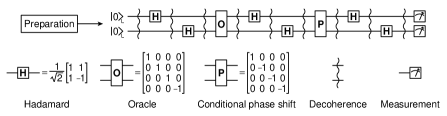
Figure 1: Running Grover’s search algorithm on an error-avoiding quantum computer. Time runs from left to right. Decoherence-free logical qubits are represented by horizontal lines. Engineered decoherence is applied at nine points during the experiment to test the computer’s resistance.

The algorithm’s purpose is to retrieve, from an unsorted list, the single item that satisfies a given criterion. Grover’s algorithm is highly efficient, requiring only $\mathcal{O}(\sqrt{N})$ steps to search a list with $N$ items; a classical algorithm requires $\mathcal{O}\left(N\right)$ steps. In our implementation of Grover’s algorithm, the logical qubit basis states $|00\rangle_{L}$, $|01\rangle_{L}$, $|10\rangle_{L}$ and $|11\rangle_{L}$ correspond to the four items in our list. We choose state $|11\rangle_{L}$ to correspond to the item we wish to retrieve. The algorithm’s first step is to prepare the register in an equal superposition of its basis states, $|\psi\rangle_{L}=(1/2)\sum_{x_{1}=0}^{1}\sum_{x_{2}=0}^{1}|x_{1}x_{2}\rangle_{L}$. The rest of the algorithm is an iterative process that increases the amplitude of the sought-after state ($|11\rangle_{L}$) until it is the dominant part of the superposition. For our two-qubit register, only one iteration is required. Finally, the logical qubits are measured; an outcome of $|11\rangle_{L}$ indicates that the algorithm has been successful. (We have also used our computer to implement the improved Deutsch-Jozsa algorithm described by Collins et al. Collins et al. (1998), with similar results.)

Our computer is based on the isotope-substituted glycine molecule shown in Fig. 2 com (c).

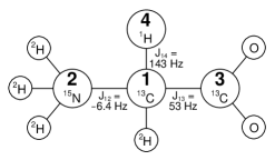
Figure 2: Isotope-substituted glycine molecule. Spin-1/2 nuclei used as physical qubits are numbered 1–4. The chemical shifts of $\mbox{}^{13}\text{C}$ spins 1 and 3 differ by 16.5 kHz on a 500 MHz ($\mbox{}^{1}\text{H}$ resonance frequency) NMR spectrometer.

Each of the molecule’s four spin-1/2 nuclei is used as a physical qubit. The errors of Eq. (1) are applied artificially according to the following protocol. At each of nine points in the experiment (indicated in Fig. 1), error operator $X_{1}X_{2}I_{3}I_{4}$ is applied with probability $e$, then error operator $I_{1}I_{2}X_{3}X_{4}$ is applied with the same probability. To simulate the effect of a microscopic random process, the experiment is performed 2048 times, each time with different randomly selected errors, and the results are averaged, giving the overall decoherence process a non-unitary, deterministic character. The resulting decoherence increases with the error probability $e$, becoming strongest at $e=0.5$. Formally, the operators describing our engineered decoherence are $E_{0}=\left(1-e\right)I_{1}I_{2}I_{3}I_{4}$, $E_{1}=\sqrt{e\left(1-e\right)}X_{1}X_{2}I_{3}I_{4}$, $E_{2}=\sqrt{e\left(1-e\right)}I_{1}I_{2}X_{3}X_{4}$, and $E_{3}=eX_{1}X_{2}X_{3}X_{4}$. (Note that for these error operators, it is clear that $\sum_{d}E_{d}\rho_{|00\rangle_{L}}E_{d}^{\dagger}=\rho_{|00\rangle_{L}}$, where $\rho_{|00\rangle_{L}}$ is defined by Eq. (3).)

We have repeated the Grover algorithm experiment in the presence of nine different levels of engineered decoherence ranging from $e=0$ to $e=0.5$. At all values of $e$, the resulting NMR spectra contain little distortion and clearly describe the final state of the qubit register as $|11\rangle_{L}$, indicating the computer has successfully executed the algorithm. To quantify the resistance of each computation to the applied decoherence, we measured the integrated absolute intensity of the final signal relative to the $e=0$ experiment. The dependence of signal intensity on $e$ is different for each of the experiment’s three temporal averaging steps and we have chosen to analyze the results of the steps separately (Fig. 3).

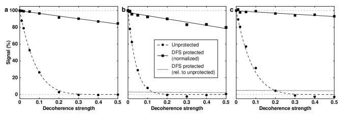
Figure 3: Experimental results in the presence of decoherence, for both the error-avoiding and unprotected computers running Grover’s algorithm. Results from the three temporal averaging steps appear separately in (a, $Z_{1}Z_{2}I_{3}I_{4}$), (b, $Z_{1}Z_{2}Z_{3}Z_{4}$), and (c, $I_{1}I_{2}Z_{3}Z_{4}$). The integrated absolute intensity of the output signal measured at the end of Grover’s algorithm is charted as a function of decoherence strength $e$. For some values of $e$, the signal from the unprotected computer is phase inverted with respect to the correct output signal: In such cases we report a negative signal intensity. Square and round points are experimental data from the error-avoiding and unprotected computers, respectively, with each dataset normalized to the intensity of its first point. Solid lines are linear regressions. Dashed curves are a theoretically predicted intensity function, $S=\left(1-2e\right)^{n}$ with $n=6$ in (a, c) and $n=12$ in (b), obtained by predicting the unprotected computer’s state at each of the experiment’s nine decoherence points and counting the number $n$ of error operators which could change the system’s state. Dotted lines are signal intensities from the error-avoiding computer normalized to the intensity of the unprotected computer’s $e=0$ signal; the signals in (a) were recorded on different nuclei and cannot be compared in this way.

We observe only small losses of signal, and these cannot be attributed to any fault in the DFS encoding. The losses are predominantly due to imperfections in pulses used to implement the engineered decoherence, evidenced by a linear decrease in signal with increasing $e$.

As a control, we have repeated these experiments on a quantum computer that does not use error avoidance. The unprotected computer is similar to the error-avoiding computer, with only the following changes: Spins 1 and 4 (Fig. 2) serve directly as qubits (in place of the two logical qubits), the temporal averaging scheme prepares a different (pseudo-pure) initial state, and different pulse sequences are used to implement quantum logic gates. The same engineered decoherence is applied and the computer executes the same algorithm as in the error-avoiding computing experiments. As expected, the unprotected computer’s signal intensity decreases rapidly with the error strength $e$. We observe effectively no signal when $e\geq 0.3$ and the result of the algorithm is incorrect or unreadable for $e\geq 0.2$.

The DFS encoding our error-avoiding computer uses has an overhead cost, but the results show it is small compared to the protection it affords. The pulse sequences that perform logical operations on the error-avoiding computer are more complex than for the unprotected control computer, so the error-avoiding computer is more vulnerable to signal loss due to pulse imperfections and natural spin relaxation. This is why, when signal intensities from the two computers are compared on an absolute scale (dotted and dashed lines in Fig. 3), the unprotected computer gives the stronger signal for low values of $e$. However, the unprotected computer consistently fails when $e\geq 0.2$, while the error-avoiding computer gives the correct result for all $e$. The overall fidelity of the Grover algorithm is governed by the temporal averaging step that is least tolerant to decoherence (Fig. 3b), and for this step the error-avoiding computer’s signal is the more intense for $e\geq$ $\sim\!\!0.15$. Even at this low level of decoherence, the protection afforded by DFS encoding outweighs the overhead involved.

In summary, we have provided the first experimental demonstration of quantum computation in the presence of strong decoherence com (a), thus proving that quantum error avoidance based on DFSs can very effectively protect qubits from decoherence during the execution of a quantum algorithm. We have implemented Grover’s search algorithm on two two-qubit quantum computers, one error-avoiding and one unprotected. While the unprotected computer fails when exposed to even a moderate amount of decoherence, the error-avoiding computer is successful in the presence of the strongest possible decoherence. This demonstration is a proof of the concept of quantum error avoidance and suggests that DFS encoding will play an important role in future experimental implementations of quantum algorithms in the presence of decoherence.