Mutual first order coherence of phase-locked lasers

Abstract

We argue that (first-order) coherence is a relative, and not an absolute, property. It is shown how feedforward or feedback can be employed to make two (or more) lasers relatively coherent. We also show that after the relative coherence is established, the two lasers will stay relatively coherent for some time even if the feedforward or feedback loop has been turned off, enabling, e.g., demonstration of unconditional quantum teleportation using lasers.

I Introduction

Recently, several authors have pointed out that although it has been known for a long time that a laser does not generate a coherent state, it is still possible to use laser light to observe phenomena that are theoretically described in terms of optical (first order) coherence Molmer ; Rudolph ; Enk ; Wiseman .

Mølmer Molmer argues that optical coherence, manifested, e.g., in a non-vanishing expectation value of the electric field operator, is a “convenient fiction” and he demonstrates that experiments that are usually interpreted in terms of optical coherence need not be described in those terms. Moreover, he argues that optical coherence is not easily generated, and in particular, that a laser does not generate coherent state. Rudolph and Sanders Rudolph show that if Mølmer’s assertions are true, so that the output state of a laser is given by the density operator

$$\hat{\rho}_{L}=\int_{0}^{2\pi}{d\phi\over 2\pi}|\alpha e^{i\phi}\rangle\langle\alpha e^{i\phi}|=e^{-\alpha^{2}}\sum_{n=0}^{\infty}{\alpha^{2n}\over n!}|n\rangle\langle n|,$$ (1)

then quantum teleportation is not possible under the conditions postulated for “unconditional quantum teleportation” Furusawa ; Braunstein . Rudolph and Sanders do not rule out the existence of sources of coherent states, but argue that lasers do not produce light with (first order) optical coherence. Van Enk and Fuchs Enk claim that while a laser does not produce optical coherence in Mølmer’s sense, subsequent temporal modes of the laser output are phase correlated. That is, if the output from a laser is expanded in subsequent orthogonal temporal modes, the state of $M$ such modes is

$$\int_{0}^{2\pi}{d\phi\over 2\pi}|\alpha e^{i\phi}\rangle\langle\alpha e^{i\phi}|^{\otimes M},$$ (2)

where the symbol ^⊗M denotes a $M$-fold tensor product. A requirement for this is that the laser’s coherence time is longer than $M$ times the time duration of a temporal mode. In such a state all the $M$ subsequent modes are first order coherent relative to each other, in contrast to the $M$-mode state $\hat{\rho}_{L}^{\otimes M}$. Both states have a vanishing expectation value of the electric field operator for all modes. Van Enk and Fuchs claim that such “phase coherence” is sufficient to allow unconditional quantum teleportation. Wiseman Wiseman , finally, asserts that there are “no devices that can generate ‘true coherence’ any better than a laser.” The basis for his claim is that any oscillator, or oscillation, can only be described relative to some accepted “clock” standard. He goes on stating that nothing suggests that there exist any better “clock” at optical frequencies than a laser. We subscribe to this view, and it is compounded by the fact that at the National Institute of Standards i Boulder, Colorado, the next generation of an “atomic clock” in development is indeed an optical clock Diddams . That is, the clock oscillator operates at an optical-, rather than a microwave-transition of an atom.

The coherent state $|e^{i\phi}|\alpha|\rangle$ of an oscillator with the angular center frequency $\omega_{0}$, can mathematically be generated from the vacuum state through the displacement operator. It is a minimum uncertainty state in the in-phase operator $\hat{a}_{1}=(\hat{a}+\hat{a}^{\dagger})/2$ and the quadrature-phase operator $\hat{a}_{2}=(\hat{a}-\hat{a}^{\dagger})/2i$, where $\hat{a}$ ($\hat{a}^{\dagger}$) is the bosonic annihilation (creation) operator. The quadrature amplitude fluctuation operators are defined $\triangle\hat{a}_{i}=\hat{a}_{i}-\langle\hat{a}_{i}\rangle$, with $i=1,2$. In Table 1 we have computed the expectation values of the quadrature amplitudes, the photon number, and their variances for the two states $\hat{\rho}_{L}$ and $|e^{i\phi}|\alpha|\rangle$ (for the particular choice $\phi=0$) in columns two and three. The table clearly shows that the observable statistics of the two states differ significantly. Hence, they cannot both describe the output of a laser, at least not if similar initial and boundary conditions for the laser and the detector are assumed. Wang et al. have also studied and quantified this difference Wang .

In the following we shall describe a simple model of phase locking of two independent lasers to a master laser. Phase-locking of two lasers has already been demonstrated using both CW Ye and pulsed lasers Shelton . However, phase-locking of two independent lasers close to the quantum limit, that is such that the relative phase fluctuations are comparable to those of two ideal coherent states, has never been demonstrated. We shall see, that it is possible to stabilize two lasers so that they are relatively first-order coherent to that extent, although they are incoherent relative to any third, auxiliary laser, or other “clock standard”. A similar proposal has also been put forth by Fujii Fujii , but in Fujii , the analysis is geared towards a practical implementation of quantum teleportation, whereas we direct our interest towards the question whether first order coherence between two lasers can be established at all.

It will be convenient to work in the Heisenberg picture in the spectral domain. Since a CW laser output consists of a continuous photon flux, we shall work with the photon flux operator $\hat{r}$. (See subsection A.1 in the Appendix for a detailed discussion of $\hat{r}$.) For a coherent state, the spectral relations corresponding to equations three and four in the third column of Table 1 are Yamamoto

$$S_{\Delta\hat{r}_{1}}(\Omega) = 1/4,$$ (3)

$$S_{\Delta\hat{r}_{2}}(\Omega) = 1/4,$$ (4)

where $\Omega=\omega-\omega_{0}$ so that, e.g., $S_{\Delta\hat{r}_{1}}(\Omega)$ is the double-sided power spectrum of $\Delta\hat{r}_{1}$ around the center frequency $\omega_{0}$. (Note that the laser external field spectra computed in Ref. Yamamoto are single-sided spectra.) These relations demonstrate a particular feature of the coherent state, namely a frequency independent quadrature amplitude noise spectrum. Operationally, this means that the quadrature amplitude noise of a coherent state is stationary. Moreover, a field in a coherent state remains in a coherent state independent of the detector temporal response function (see the Appendix).

The corresponding spectra for the laser external field have also been computed in Yamamoto . While the model employed was specifically targeting a semiconductor laser, the general features are largely independent of the laser type. It was found that the corresponding relations for (a somewhat idealized) laser, pumped high above the threshold, are

$$S_{\Delta\hat{r}_{1}}(\Omega) = 1/4~{}\text{and}$$ (5)

$$S_{\Delta\hat{r}_{2}}(\Omega) = {\Omega^{2}+\gamma^{2}\over 4\Omega^{2}},$$ (6)

where $\gamma$ is the inverse of the laser photon lifetime. We see that (6) radically differs from (4) in that Eq. (6) has a $1/\Omega^{2}$ behavior at low frequencies. This is characteristic of a Wiener process, leading to diffusion. Therefore, even if the phase of the external field amplitude was known (e.g., through a series of measurements) at some time $t_{0}$, the phase will be randomized through phase diffusion at times $t\gg t_{0}+1/\gamma$. Therefore, unless the field of the laser has been measured relative to a reference within the laser’s coherence time $1/\gamma$, the state of a laser is well described by the density operator $\hat{\rho}_{L}$ irrespective of how relatively stable the reference oscillator is. The density matrix $\hat{\rho}_{L}$ also describes the state of a free-running laser, that is, a laser whose phase relative to our reference is unknown. This result is indeed expected from symmetry arguments, and Mølmer, in particular, emphasize that there is no mechanism in a free-running laser that breaks the in-phase, quadrature-phase symmetry. Hence, the expectation value of the electric field of an unmonitored, free-running laser vanishes.

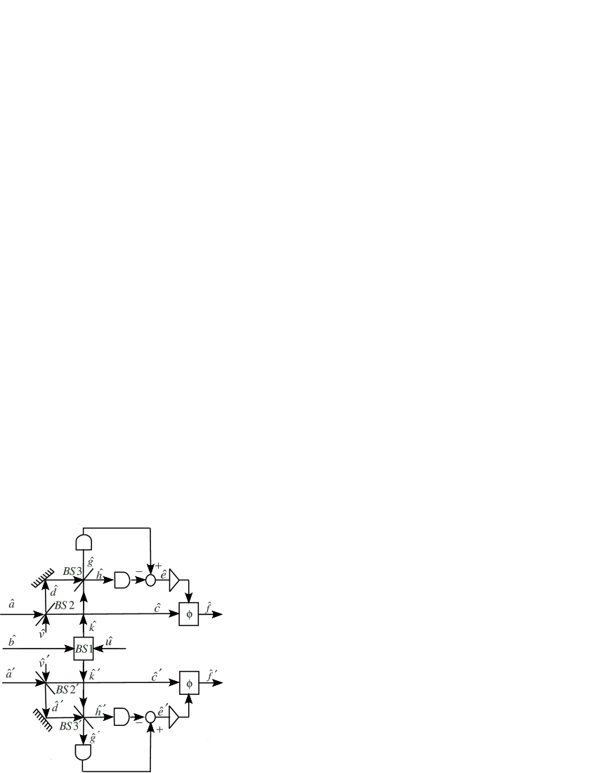
Figure 1: A schematic drawing of two lasers locked by feedforward to a master oscillator laser.

II Phase-locked lasers

Now consider the case when we stabilize the laser field with the help of a master oscillator. In the following we will consider feedforward stabilization, for simplicity. Later, we shall briefly discuss feedback stabilization. Fig. 1 shows a schematic drawing of two lasers locked to a master oscillator by feedforward. The notation we will use is defined by the figure. The master oscillator (laser) field $\hat{b}$ is divided into two by beam splitter one (BS1) which is a 50/50 beam splitter. The field into the other port of the beam splitter is a vacuum field $\hat{u}$, so that the beam splitter output modes $\hat{k}$ and $\hat{k}^{{}^{\prime}}$ are given by $\hat{k}=\frac{1}{\sqrt{2}}(\hat{b}+\hat{u})$ and $\hat{k}^{{}^{\prime}}=\frac{1}{\sqrt{2}}(\hat{b}-\hat{u})$.

Next, we look at beam splitter two (BS2), where part of the laser field $\hat{a}$ is tapped to get a locking signal $\hat{d}$. Again, a vacuum field, denoted $\hat{v}$, is incident on the other input port. Hence, the two output fields $\hat{d}$ and $\hat{c}$ are given by

$$\hat{d}=r\hat{a}+t\hat{v},~{}\text{and}~{}\hat{c}=t\hat{a}-r\hat{v},$$ (7)

where $r=\sin\theta$ ($t=\cos\theta$) is the reflectivity (transmissivity) of the beam splitter. At beam splitter number three (BS3), which is also a 50/50 splitter, the fields $\hat{d}$ and $\hat{k}$ are mixed, and subsequently the outputs $\hat{g}$ and $\hat{h}$, which are given by

$$\hat{g}=(\hat{d}+\hat{k})/\sqrt{2}=(r\hat{a}+t\hat{v})/\sqrt{2}+\frac{1}{2}(\hat{b}+\hat{u})$$ (8)

and

$$\hat{h}=(\hat{d}-\hat{k})/\sqrt{2}=(r\hat{a}+t\hat{v})/\sqrt{2}-\frac{1}{2}(\hat{b}+\hat{u})$$ (9)

are measured by photodetectors. The detector photocurrents will be proportional to $\hat{g}^{\dagger}\hat{g}$ and $\hat{h}^{\dagger}\hat{h}$, that can be expressed as

$$\hat{g}^{\dagger}\hat{g}=(\hat{d}^{\dagger}\hat{d}+\hat{d}^{\dagger}\hat{k}+\hat{k}^{\dagger}\hat{d}+\hat{k}^{\dagger}\hat{k})/2$$ (10)

and

$$\hat{h}^{\dagger}\hat{h}=(\hat{d}^{\dagger}\hat{d}-\hat{d}^{\dagger}\hat{k}-\hat{k}^{\dagger}\hat{d}+\hat{k}^{\dagger}\hat{k})/2.$$ (11)

The difference between the measured photocurrents $\hat{g}^{\dagger}\hat{g}-\hat{h}^{\dagger}\hat{h}$ will be the homodyne signal $\hat{e}$, which we call the error signal. This signal is simply

$$\hat{e}=\hat{d}^{\dagger}\hat{k}+\hat{k}^{\dagger}\hat{d}.$$ (12)

Now, expand the operators in quadrature components and assume that $\hat{d}$ leads $\hat{k}$ by the relative phase angle $\pi/2$. (this choice of relative phase will beat the excitation of one field with the quadrature amplitude of the other field.) That is, we multiply the operator $\hat{d}$ with $\exp(i\pi/2)=i$ and remember that both fields are expressed relative to the same fiducial field. (Below, we shall see that the relative phase angle $\pi/2$ is the stable feedforward locking point.) This will yield the mean error signal zero, and the fluctuating part of the error signal will be

$$\hat{e} = -i(d_{0}+\triangle\hat{d}_{1}-i\triangle\hat{d}_{2})(k_{0}+\triangle\hat{k}_{1}+i\triangle\hat{k}_{2})$$ (14)

$$+i(k_{0}+\triangle\hat{k}_{1}-i\triangle\hat{k}_{2})(d_{0}+\triangle\hat{d}_{1}+i\triangle\hat{d}_{2})$$

$$= 2(d_{0}\triangle\hat{k}_{2}-k_{0}\triangle\hat{d}_{2})+\mathcal{O}(\triangle^{2}),$$ (15)

where $\mathcal{O}(\triangle^{2})$ denotes terms of second order in the quadrature flux fluctuation operators.

It is well worth examining Eq. (15) in some detail, since it is the generic noise equation for homodyne measurements. Assume, that each of the fields $\hat{k}$ and $\hat{d}$ is in a coherent state. Hence, it follows that the two fields are relatively coherent. Since the quadrature amplitude fluctuations of a coherent state are equal, and independent of the state’s excitation, the homodyne detection noise is dominated by the weaker field, since the weaker field’s quadrature amplitude noise beats against the stronger field’s in-phase amplitude. (It is customary to refer to the stronger field as the “local oscillator.”) If the two fields have unequal quadrature amplitude fluctuations, e.g., assume that $S_{\triangle\hat{k}_{2}}(\Omega)>S_{\triangle\hat{d}_{2}}(\Omega)$, then the homodyne detection noise is still dominated by the quadrature amplitude fluctuations of $\hat{d}$ provided that $k_{0}^{2}>d_{0}^{2}S_{\triangle\hat{k}_{2}}(\Omega)/S_{\triangle\hat{d}_{2}}(\Omega)$.

Using the relations between incident and output fields above, we can re-express this equation in the (quadrature expansion of the) input fields $\hat{a}$, $\hat{b}$, $\hat{u}$, and $\hat{v}$. The result (to first order in the fluctuation operators) is

$$\hat{e}=\frac{ra_{0}}{\sqrt{2}}(\triangle\hat{b}_{2}+\triangle\hat{u}_{2})-\frac{b_{0}}{\sqrt{2}}(r\triangle\hat{a}_{2}+t\triangle\hat{v}_{2}).$$ (16)

This is almost what we desire. Remember that the objective is to reduce the large fluctuations of $\triangle\hat{a}_{2}$ at low frequencies. These are the fluctuations leading to phase diffusion. The error signal clearly contain the information about these fluctuations. By making the master oscillator flux amplitude sufficiently large, so that $b_{0}$ is much larger than $a_{0}$, this noise information will dominate the error signal at low frequencies. (Remember that the spectral density of $\triangle\hat{a}_{2}$ and $\triangle\hat{b}_{2}$ increases as $\Omega^{-2}$, whereas the spectral density of $\triangle\hat{u}_{2}$ and $\triangle\hat{v}_{2}$ is 1/4, independent of frequency.) From the expression (16) we see that under this condition, if the relative phase between $\triangle\hat{a}_{2}$ and $\triangle\hat{b}_{2}$ is larger than $\pi/2$, that is, either $\triangle\hat{a}_{2}$ is positive or $\triangle\hat{b}_{2}$ is negative, then the error signal is negative. In order to compensate for the $\triangle\hat{a}_{2}$ fluctuations, the error signal should be feed forward, keeping the sign, to a phase shifter. Let us, therefore, see what happens when we apply some phase shift, say $\phi$, to an output signal $\hat{c}=c_{0}+\triangle\hat{c}_{1}+i\triangle\hat{c}_{2}$. In this case we denote the phase shifted signal by $\hat{f}$

$$\hat{f} = \exp(i\phi)\hat{c}$$ (17)

$$= (c_{0}+\triangle\hat{c}_{1})\cos\phi-\triangle\hat{c}_{2}\sin\phi$$ (19)

$$+i[\triangle\hat{c}_{2}\cos\phi+(c_{0}+\triangle\hat{c}_{1})\sin\phi]$$

$$\approx c_{0}+\triangle\hat{c}_{1}+i(\triangle\hat{c}_{2}+c_{0}\phi),$$ (20)

where we have linearized the equation to first order in $\phi$, $\triangle\hat{c}_{1}$, and $\triangle\hat{c}_{2}$. Assume now that the phase shift $\phi$ is equal to the error signal $\hat{e}$ times some feedforward gain ${\cal G}$. The output signal after phase correction by the error signal is given by

$$\hat{f}\approx t(a_{0}+\triangle\hat{a}_{1}+i\triangle\hat{a}_{2})-r(\triangle\hat{v}_{1}+i\triangle\hat{v}_{2})+ita_{0}{\cal G}\hat{e}.$$ (21)

To cancel the noise term $\triangle\hat{a}_{2}$ in the expression above, we have to adjust the feedforward gain so that

$${\cal G}=\sqrt{2}/ra_{0}b_{0}.$$ (22)

After doing so, the output signal becomes

$$\hat{f}=ta_{0}+t\triangle\hat{a}_{1}-r\triangle\hat{v}_{1}+i\left[\frac{ta_{0}}{b_{0}}(\triangle\hat{b}_{2}+\triangle\hat{u}_{2})-\frac{1}{r}\triangle\hat{v}_{2}\right],$$ (23)

where we have used the relation $t^{2}+r^{2}=1$. From this equation we see that the noise term $\triangle\hat{a}_{2}$, describing the phase-diffusion noise originating in the laser generating the $\hat{a}$ field, is absent. Instead, a new diffusion noise term $ta_{0}\triangle\hat{b}_{2}/b_{0}$ has appeared. Since the master oscillator is also a laser, this noise term will also have a spectral density proportional to $\Omega^{-2}$ at low frequencies. Hence, one Wiener process, $\triangle\hat{a}_{2}$ (relative to the fiducial reference), has simply been replaced by another, $\triangle\hat{b}_{2}$.

Let us now see what happens with the output field $\hat{f}^{{}^{\prime}}$ if we subject the laser field $\hat{a}^{{}^{\prime}}$ to the same sequence of measurement and feedforward as the field $\hat{a}$. The calculation of $\hat{f}^{{}^{\prime}}$ proceeds in a similar fashion as for $\hat{f}$, except that the field $\hat{k}^{{}^{\prime}}=(\hat{b}-\hat{u})/\sqrt{2}$. Hence, the only difference from the expression (23) above is that all fields should be primed, except for the master oscillator field $\hat{b}$ and the vacuum field operator $\hat{u}$. However, the sign in front of the operator $\hat{u}$ should be reversed. Hence, the output $\hat{f}^{{}^{\prime}}$ becomes

$$\hat{f}^{{}^{\prime}}=ta_{0}^{{}^{\prime}}+t\triangle\hat{a}^{{}^{\prime}}_{1}-r\triangle\hat{v}^{{}^{\prime}}_{1}+i\left[\frac{ta_{0}^{{}^{\prime}}}{b_{0}}(\triangle\hat{b}_{2}-\triangle\hat{u}_{2})-\frac{1}{r}\triangle\hat{v}^{{}^{\prime}}_{2}\right].$$ (24)

Assume that the two field amplitudes $ta_{0}$ and $ta_{0}^{{}^{\prime}}$ are equal and that the two fields $\hat{f}$ and $\hat{f}^{{}^{\prime}}$ are detected by a balanced homodyne detector. The detector output, that is the beat-note between the two incident fields $\hat{f}$ and $\hat{f}^{{}^{\prime}}$, can then be deduced in a straightforward fashion by comparing with (15). The detector output fluctuations will be

$$f_{0}\triangle\hat{f}^{{}^{\prime}}_{2}-f_{0}^{{}^{\prime}}\triangle\hat{f}_{2}=2ta_{0}\left(\frac{2ta_{0}\triangle\hat{u}_{2}}{b_{0}}+\frac{\triangle\hat{v}^{{}^{\prime}}_{2}-\triangle\hat{v}}{r}\right).$$ (25)

From this equation we see that the relative-noise spectrum is no longer proportional to $\Omega^{-2}$ at low frequencies, but is flat, since $\triangle\hat{u}_{2}$, $\triangle\hat{v}_{2}$ and $\triangle\hat{v}^{{}^{\prime}}_{2}$ all emanate from vacuum fluctuations and hence have frequency independent spectra with the spectral density 1/4. Recalling that an earlier assumption was that $b_{0}\gg a_{0}$, the first term on the right hand side of (25) can be neglected. Therefore, the spectral density of the detector fluctuations is, to a good approximation, $2(ta_{0}/r)^{2}$ at all frequencies (see the Appendix). In comparison, the homodyne detector spectra from two coherent states, with field amplitudes $ta_{0}$, would be $2(ta_{0})^{2}$. Hence, as $r\rightarrow 1$, the relative quadrature-phase noise of the two locked lasers will approach the noise level of two coherent state sources. At the same time, the mean in-phase amplitude of $\hat{f}$ and $\hat{f}^{{}^{\prime}}$ would approach zero. Assume now that we use the relatively coherent fields $\hat{f}$ and $\hat{f}^{{}^{\prime}}$ as local oscillators in two separate homodyne measurements. Using (15), it is not difficult to prove that in order to minimize the influence of the local oscillator quadrature amplitude noise, the choice $t=r=2^{-1/2}$ should be made. Assume, for simplicity, that the field we want to measure is a coherent state with mean amplitude $d_{0}$. If so, the coherent state’s quadrature amplitude noise will dominate the measurement fluctuations if $a_{0}>2d_{0}$. That is, with this choice of mirror transmission $t$, the two fields $\hat{f}$ and $\hat{f}^{{}^{\prime}}$ are relatively coherent, each with a noise spectral density twice of that of a coherent state. For a more detailed discussion of the connection between (25) and the first order coherence function between the locked lasers, the reader is referred to the Appendix, subsection A.3.

An additional consequence, discussed in more detail in subsection A.2 in the Appendix, is that within a time small compared to the inverse spectral linewidth of the locked lasers, the lasers will remain relatively coherent even if the feedforward locking loop is turned off. It will thus be possible to do, e.g., continuous variable teleportation without giving up the quantum teleportation criteria given in Braunstein

III Feedforward v.s. feedback

Above, we have analyzed the situation where two lasers are phase locked to a third laser by feedforward. While such a scheme lends itself to a simple analysis, the scheme has obvious practical shortcomings. One is the need of a precise control of the feedforward gain. In order to completely suppress the phase diffusion of each laser, relative to the master laser, the feedforward gain must be precisely set according to (22). This will be impossible in reality. In addition, the mean absolute value of the error signal (16) will be grow with time as $t^{1/2}$, there $t$ is the time since the main information the error signal contains, $\triangle\hat{a}_{2}$, is a non-stationary term. The error signal is used to drive a phase-compensating device, e.g., an electrooptical crystal or an adjustable piezoelectrically controlled delay line. However, due to the fact that with time, the error signal will increase without limit, any phase-compensating device will eventually run out of range and will have to be reset.

In reality, it would be wiser to lock the lasers by feedback, and the feedback should act on the laser frequency (e.g., translating one of the laser’s mirrors) after appropriate filtering. In a feedback loop, the relative fluctuations will initially become smaller and smaller with increasing feedback gain. If the feedback measurement and feedback loop is carefully designed, it is possible to reach the limit set by quantum noise manifested in (25) before (non-fundamental) feedback loop fluctuations are sufficiently amplified to dominate the locked lasers’ output. In addition, since the accumulated relative phase equals the time integrated frequency difference between the master and slave laser, the phase-compensating device will not run out of range. Differently stated, the lasers frequency difference is the time derivative of the lasers’ relative phase. Therefore, if the latter noise process has a spectrum proportional to $\Omega^{-2}$, the former noise has a flat spectrum at low frequencies. The frequency error signal is hence a stationary process. Hence, if the feedback is implemented by moving one of the laser’s mirrors, its position needs only to be adjusted within a fixed range and the actuator moving the mirror need not run out of range.

The disadvantage with feedback locking is that it is more difficult to analyze, and that one risks self oscillation at baseband frequencies $\Omega$ where $\Omega\tau_{f}=\pi$. Here, $\tau_{f}$ is the feedback loop time delay. At this frequency the feedback loop does no longer suppress the fluctuation but instead enhances them. If the feedback loop gain is too high, one induces self oscillation. Hence, one needs to make a compromise between the feedback loop stability and the feedback gain, all while maximizing the feedback loop bandwidth. Since our analysis essentially only had the purpose to point out that coherence of a harmonic oscillator must always be relative to some reference oscillator, we will not delve deeper into these issues here.

IV Conclusions

We have argued that first order coherence is a relative property, and that if one accepts this view, the light emanating from a laser can be first-order coherent relative to itself at an earlier time, or to a different laser. Due to phase diffusion, two lasers will only stay relatively coherent for a time smaller than the smallest of inverses the lasers’ respective linewidth unless they are actively phase-locked. Since, in principle, the laser linewidth can be as small as one wishes, this fact does not prevent lasers to be used to demonstrate, e.g., unconditional quantum teleportation. It could in principle be done by locking Alice’s and Bob’s homodyning lasers to a master laser before the unknown state and the shared entangled are measured with the help of the laser. The locking is then turned off, and Alice’s and Bob’s respective laser become free running. The two experimentalists now have roughly the lasers’ coherence time to perform the teleportation, including the Alice’s homodyne measurements, the classical communication, and the final unitary evolution by Bob. A typical laser’s coherence time may seem short on the human time-scale ($\sim$1 s). However, on an electronics time-scale ($\sim$1 ns), a two good lasers stay relatively coherent for a long time.

In the Appendix, we have included a discussion why the popular model of laser fluctuations using Langevin noise sources fail to describe the laser’s behavior for times long compared to the laser’s inverse linewidth. The linearization customarily employed in the solution of these equations neglect to take the restoring force of the quadrature-phase amplitude fluctuations in account, and hence these equations erroneously predicts that it is only the quadrature-phase amplitude, relative to some fix fiducial reference, that diffuses. Unfortunately, if the equations are not linearized, they are difficult to solve analytically.

Appendix A Expectation values from flux spectra

A.1 Expectation values of a coherent state

Here we derive the relation between the external field operator $\hat{r}$ and the mean photon number and the photon number variance of a specific mode. The external field operator $\hat{r}$ correspond to a photon flux amplitude. The photon flux operator is hence given by $\hat{r}^{\dagger}\hat{r}$, and has the unit Hz. The expectation value of $\hat{r}^{\dagger}\hat{r}$ gives the mean photon flux, in photons per second. Let us expand $\hat{r}$ relative some fiducial reference as $\hat{r}(t)=r_{0}+\Delta\hat{r}_{1}(t)+i\Delta\hat{r}_{2}(t)$. Here, the field amplitude $r_{0}$ has been assumed to be in phase with a fiducial reference. Expanding to first order in the fluctuation operators $\Delta\hat{r}_{1}(t)$ and $\Delta\hat{r}_{2}(t)$ we get

$$\hat{r}^{\dagger}\hat{r}\approx r_{0}^{2}+2r_{0}\Delta\hat{r}_{1}(t).$$ (26)

Assume now that a photodetector temporal mode-function $h$ is a rectangle function of duration $T$, see Fig. 2. The detector output, as a function of time, will be the convolution between the flux and the detector response function

$$R(t)=(\hat{r}^{\dagger}\hat{r})\ast h\approx[r_{0}^{2}+2r_{0}\Delta\hat{r}_{1}(t)]\ast h.$$ (27)

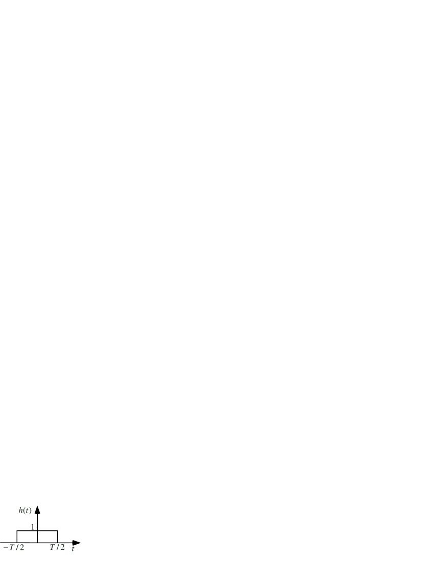
Figure 2: The assumed temporal mode function.

Sampling this function every $T$ seconds, yields the photon number in subsequent orthogonal temporal modes. The detected mean photon number per mode hence becomes

$$\langle\hat{n}\rangle=r_{0}^{2}T.$$ (28)

We would now like to compute the photon number variance of such a mode. Since the coherent field flux fluctuations are ergodic we can proceed as follows: Define $y(t)=\Delta\hat{r}_{1}(t)\ast h$. The spectral density of this signal is

$$S_{y(t)}(\Omega)=S_{\hat{r}_{1}(t)}|H(\Omega)|^{2}={1\over 4}|H(\Omega)|^{2},$$ (29)

where the spectral filter function $H(\Omega)$ is the Fourier transform of $h$ and we have used the fact that the spectral density of the quadrature amplitude fluctuations of a coherent state flux is 1/4 according to (3). The first order correlation function $G(\tau)$ of $y(t)$ is the (inverse) Fourier transform of its power spectrum, so that

$$G_{y(t)}(\tau)={\cal F}^{-1}S_{y(t)}(\Omega)={1\over 4}h\ast h,$$ (30)

where we have used the fact that the Fourier transform of a product of functions is the convolution of their respective inverses. Finally, the variance of $y(t)$ is $G_{y(t)}(0)$. Looking at figure 3, we find that $G_{y(t)}(0)=T/4$. This means that the photon number variance can be expressed

$$\langle\Delta\hat{n}^{2}\rangle=4r_{0}^{2}\langle(\Delta\hat{r}_{1}(t))\ast h)^{2}\rangle=4r_{0}^{2}T/4=Tr_{0}^{2}.$$ (31)

Comparing with (28) we see that we arrive at the expected result for a coherent state.

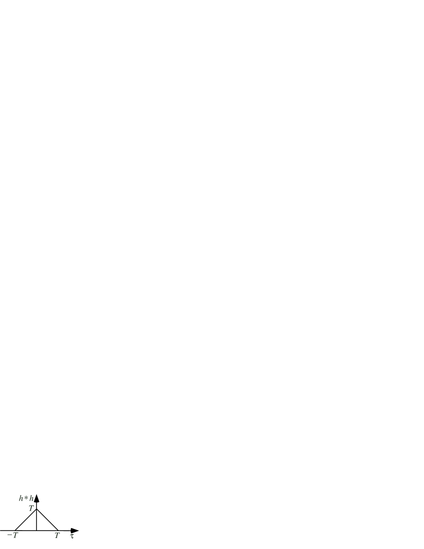
Figure 3: The temporal mode function convolution.

To derive the mean quadrature amplitudes and their variances we proceed in a similar way. Suppose two fields, characterized by the photon flux amplitudes $\hat{r}$ and $\hat{r}^{{}^{\prime}}$ are incident on a homodyne detector. If the two fields are relatively coherent and have the same phase, we can use (12) and insert the expansion of the fields in quadrature amplitude components (e.g., $\hat{r}=r_{0}+\triangle\hat{r}_{1}+i\triangle\hat{r}_{2}$). To the first order in the fluctuation operators the detector output becomes:

$$2r_{0}r_{0}^{{}^{\prime}}+r_{0}\triangle\hat{r}^{{}^{\prime}}_{1}+r_{0}^{{}^{\prime}}\triangle\hat{r}_{1}+O(\triangle^{2}).$$ (32)

Passing this signal trough appropriate detector filter, (integrate for $T$ seconds and then dump), the mean detection signal becomes

$$2r_{0}r_{0}^{{}^{\prime}}T.$$ (33)

The prefactor 2 in the equation above is simply a scaling factor. Since the signal emanates from the projection of one in-phase amplitude on another, we conclude from the symmetry of the problem that, for the field $\hat{r}$,

$$\langle\hat{a}_{1}\rangle=\sqrt{T}r_{0}$$ (34)

(Remember that, e.g., $\hat{a}_{1}$ is the in-phase amplitude of the field in a specific temporal mode, while $\hat{r}_{1}$ is the in-phase amplitude operator of a continuous flux.) Assume now that $\hat{r}^{{}^{\prime}}$ has a much larger mean in-phase amplitude than $\hat{r}$. Filtering away the DC-component of the signal (32), and measuring the variance of the detector signal after filtering the temporal mode, the detector signal approximately becomes

$$r_{0}^{{}^{\prime}}\triangle\hat{r}_{1}\ast h(t)$$ (35)

Using the same procedure as we used to compute the mean photon flux above, we see that the variance of this signal is $(r_{0}^{{}^{\prime}})^{2}T/4$. From this we can conclude that $\langle\triangle\hat{a}_{1}^{2}\rangle=1/4$, since $T(r_{0}^{{}^{\prime}})^{2}$ is the square of the mean local oscillator in-phase amplitude (the amplitude we beat the fluctuations against).

If we phase rotate $\hat{r}$ with $\pi/2$ with the respect to $\hat{r}^{{}^{\prime}}$, and follow the same procedure to calculate $\langle\hat{a}_{2}\rangle$ and $\langle\triangle\hat{a}_{2}^{2}\rangle$, we will find that $\langle\hat{a}_{2}\rangle=0$ and $\langle\triangle\hat{a}_{1}^{2}\rangle=1/4$. Hence, the results in the third column of Table 1 are reproduced if Eq. (3) and (4) are used.

A.2 Expectation values of the laser output field

If we now use (5) and (6), modelling the noise properties of the output field from a laser, we will get identical results as those in the previous subsection for $\langle\hat{n}\rangle$, $\langle(\triangle\hat{n})^{2}\rangle$, $\langle\hat{a}_{1}\rangle$, $\langle\hat{a}_{2}\rangle$, and $\langle\triangle\hat{a}_{1}^{2}\rangle$. However, due to the spectrum (6) of $\hat{r}_{2}$, the expectation value of $\langle\triangle\hat{a}_{2}^{2}\rangle=\infty$ independent of $T$.

To study this divergence, due to the diffusion of $\hat{r}_{2}$, assume that we homodyne the field $\hat{r}$ in two orthogonal temporal modes defined by two rectangle functions with durations from $t$ to $t+T$, and $t+\tau$ to $t+\tau+T$, respectively, where $\tau\geq T$. A schematic procedure to make such a measurement with the aid of a flip mirror is depicted in Fig. 4. From (15) we find that the measurement output will become $2r_{0}[\triangle\hat{r}_{2}(t)-\triangle\hat{r}_{2}(t+\tau)]\ast h(t)$. With the help of (6), the spectrum of the output fluctuations can be computed to be

$$S_{Hom}(\Omega)=4\rm^{2}\frac{\Omega^{2}+\gamma^{2}}{\Omega^{2}}\left[\frac{sin(\Omega\tau/2)sin(\Omega T/2)}{\Omega/2}\right]^{2}$$ (36)

Transforming this function back to the time domain gives the correlation function, and its value at the origin, the variance, can be computed to be:

$$r_{0}^{2}T\left[2-T\tau\gamma^{2}(1-\frac{T}{6\tau})\right].$$ (37)

We see that since $\tau\geq T$, the variance will approximately be $2r_{0}^{2}T$ (the shot noise associated with the total detected photon number $2r_{0}^{2}T$) when $T\tau<\gamma^{-2}$. That is, for measurements, even relative measurements, within the laser coherence time $\gamma^{-1}$, the laser output field in a succession of temporal modes will, each one, approximately be in a coherent state if the first mode in the succession is used as the reference. Note that this conclusion holds irrespective of the numerical values of $T$, $\tau$, and $\gamma^{-1}$ as long as $T<\tau<\gamma^{-1}$. This result agrees with the analysis of van Enk and Fuchs Enk .

A.3 First order coherence of phase-locked lasers

The first order correlation function between two classical electromagnetic fields is defined

$$\langle E({\bf\bar{r}},t)E^{\prime\ast}({\bf\bar{r}}^{\prime},t^{\prime})\rangle,$$ (38)

where ${\bf\bar{r}}$ and ${\bf\bar{r}}^{\prime}$ denote two spatial locations, and $t$ and $t^{\prime}$ denote two times. In the following we will restrict ourselves to single mode fields, and therefore, we can suppress the spatial coordinates. Expressing the fields in terms of amplitude and phase, and expanding the amplitude in its (real and positive) mean $E_{0}$, and its fluctuation around this mean $\Delta E(t)$, one gets

$$\langle E(t)E^{\prime\ast}(t^{\prime})\rangle\approx E_{0}E_{0}^{\prime}e^{i\omega_{0}(t-t^{\prime})}\langle e^{i[\phi(t)-\phi^{\prime}(t^{\prime})]}\rangle,$$ (39)

where we have dropped the term quadratic in the the fluctuations $\Delta E$, and where we have assumed that the amplitude- and the phase-fluctuations are uncorrelated. (The latter assumption is not true in semiconductor lasers, where the so-called $\alpha$-parameter characterizes the inverted-media meditated correlations between amplitude and phase. For small fluctuations this fact is inconsequential for what follows.) From Eq. (39) we see that as long as $|\phi(t)-\phi^{\prime}(t^{\prime})|\ll 1$ rad, then the correlation function has the modulus $|E_{0}E_{0}^{\prime}|$, indicating that the two fields are first order coherent. Assume that the difference $|\phi(t)-\phi^{\prime}(t^{\prime})|$ is small. We can then take either field and make it our fiducial reference, so that we work in a frame rotating with the angular frequency $\omega_{0}$. We find that in this rotating frame, $E_{0}\leftrightarrow r_{0}$, $\triangle E(t)\leftrightarrow\triangle\hat{r}_{1}$, and for small angles we have $\phi(t)\leftrightarrow\triangle\hat{r}_{2}/r_{0}$. Similar relations hold for the primed field. Hence, if we can show that for two locked lasers the relation

$$|\triangle\hat{r}_{2}/r_{0}-\triangle\hat{r}_{2}^{\prime}/r_{0}^{\prime}|\ll 1$$ (40)

holds, then our assumptions above hold, and the laser fields will be first order coherent. For two lasers with equal fields, $r_{0}=r_{0}^{\prime}$, the condition can be reformulated

$$|\triangle\hat{r}_{2}-\triangle\hat{r}_{2}^{\prime}|\ll r_{0}.$$ (41)

Hence, the homodyne measurement beat signal is directly relevant to the two fields’ relative first order coherence.

From (25) we can deduce that the noise spectrum of $\triangle\hat{r}_{2}-\triangle\hat{r}_{2}^{\prime}$ equals $4$, where we have assumed a mirror reflectivity of 1/2 for the beam splitters $BS2$ and $BS2^{\prime}$. This corresponds to an equivalent photon flux amplitude of the order 1 Hz^1/2, very much below a typical laser. E.g., a single (transverse) mode laser emitting 1 mW optical power at a wavelength of 500 nm has a photon flux amplitude of $5\cdot 10^{7}$ Hz^1/2 demonstrating that (41) is easily met. This proves the validity of our approach.

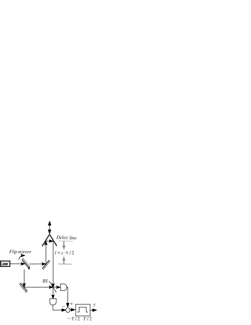
Figure 4: Schematic drawing of a homodyne measurement of different temporal modes of a laser’s output flux. The flip mirror is synchronized with the detector, and the separation between the temporal mode can be varied through the time delay $\tau=2l/c$, where $l$ is the length of the time-delay “trombone” and $c$ is the phase-velocity.

A.4 Laser potentials and the linearized approximation

To see why the noise spectra (5), (6) correctly predicts the short-time ($T$, $\tau<\gamma^{-1}$) relative-coherence properties of a laser, but fails to reproduce the long term quadrature phase properties (popularly speaking, these are called the coherence properties) manifested in the first column in Table 1, it is instructive to look at the laser potential models that underlies the various theories.

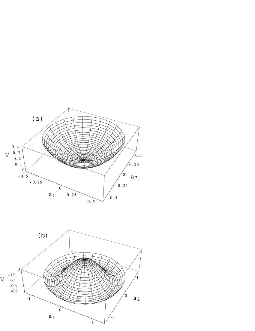
Figure 5: A laser potential with $\gamma_{0}=1$ per unit time and $C=0.8$. (a) Below threshold pumping ($\alpha=0$). (b) Above threshold pumping ($\alpha-\gamma_{0}=1.6$ per unit time).

The internal field of a laser, under certain approximations can be modelled as a particle in a particular potential subjected to Langevin noise forces. The simplest standard model for the potential, derived from the equation of motion of the field is

$$V(\hat{a})=-(\frac{\alpha-\gamma_{0}}{4})|\hat{a}|^{2}+\frac{C}{4}|\hat{a}|^{4},$$ (42)

where $\alpha$ is the overall gain per unit time in the laser, $\gamma_{0}$ the cavity decay rate (the inverse of the (cold) laser cavity photon lifetime), and $C$ is the gain saturation parameter. In Fig. 5 we see how the potential goes from a parabolic potential to a “Mexican hat” potential as the gain goes from subthreshold to above threshold. In both cases the potential has circular symmetry around the origin. Since lasing is triggered by spontaneous emission (that is one of the origins of the Langevin noise sources in the model), the laser field will not have any preferred phase (relative to the fiducial reference defining the coordinate system orientation). Therefore, a free-running laser where only the intensity is known (supposedly through a photon number measurement or by knowledge of the relation between the pumping and the output intensity) must be described by the density operator $\hat{\rho}_{L}$ of Eq. (1). As Mølmer Molmer , and other’s before him, have pointed out, a laser does not induce any symmetry breaking, and therefore it does not induce coherence relative to any other oscillator.

However, as the analysis above indicate, by measuring and influencing the field of a laser, either with feedforward control, or feedback control, the relative phase of two lasers can be locked so that the lasers become relatively coherent. However, if the locking servo is turned off, the Langevin fluctuations of each laser will make the relative phase between the two lasers diffuse, since the potential offers only a restoring force in the radial direction, but not in the azimuthal direction. After a time approximately equal to the inverse of the laser emission spectral linewidth, the two lasers are no longer relatively coherent.

This situation is not well described by Eqs. (5) and (6), because these equations predict that it is only the $\hat{a}_{2}$ quadrature that diffuses. If that were the case, then the relative phase of the two lasers with the initial relative phase zero, would remain zero, on average, for all subsequent times. If so, the quadrature-phase amplitude fluctuation would eventually become larger than the mean in-phase component. However, this is not what happens in a laser. The reason for the erroneous prediction of (6) is that in the analysis leading to the equation, the laser potential (or rather the Langevin noise operators) have been linearized about the operating point. The corresponding linearized potential is illustrated in Fig. 6. One can see that in the linearized potential, the gain saturation will only act in the direction parallel to the field expectation value. In contrast, the better model of the potential will act in the direction parallel to the instantaneous field, i.e., in the radial direction. The linearized potential correctly predicts the laser behavior for times up to the laser’s relative decoherence time, but fails for long time scales, where it is actually the relative phase, and not the quadrature field amplitude that diffuses.

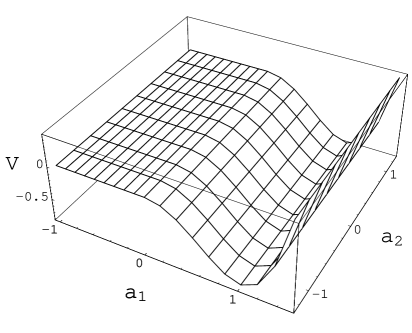
Figure 6: A linearized laser potential above threshold

	$\hat{\rho}_{L}$	$|e^{i\phi}\alpha\rangle$	Laser model
$\langle\hat{a}_{1}\rangle$	0	$|\alpha|$	$\sqrt{T}r_{0}$
$\langle\hat{a}_{2}\rangle$	0	$0$	$0$
$\langle\Delta\hat{a}_{1}^{2}\rangle$	$\frac{2|\alpha|^{2}+1}{4}$	1/4	$1/4$
$\langle\Delta\hat{a}_{2}^{2}\rangle$	$\frac{2|\alpha|^{2}+1}{4}$	1/4	$\infty$
$\langle\hat{n}\rangle=\langle\hat{a}^{\dagger}\hat{a}\rangle$	$|\alpha|^{2}$	$|\alpha|^{2}$	$Tr_{0}^{2}$
$\langle(\triangle\hat{n})^{2}\rangle$	$|\alpha|^{2}$	$|\alpha|^{2}$	$Tr_{0}^{2}$

Table 1: A table comparing the predicted statistics of three different fields. A totally statistically mixed state with Poissonian statistics, a coherent state, and the predicted output of a laser using Langevin equations.

References

- (1) K. Mølmer, Phys. Rev. A 55, 3195 (1997).
- (2) T. Rudolph and B. C. Sanders, Phys. Rev. Lett. 87, 077903 (2001.
- (3) S. J. van Enk and C. A. Fuchs, Phys. Rev. Lett. 88, 027902 (2002). S. J. van Enk and C. A. Fuchs, Quantum Info. Comp. 2, 151 (2002).
- (4) H. M. Wiseman, arXiv quant-ph/0209163 (2002).
- (5) A. Furusawa et al., Science 282, 706 (1998).
- (6) S. L. Braunstein et al., J. Mod. Opt. 47, 267 (2000).
- (7) S. A. Diddams et al, Science 293, 825 (2001).
- (8) J. Ye and J. L. Hall, Opt. Lett. 24, 1838 (1999).
- (9) R. K. Shelton et al., Science 293, 1286 (2001).
- (10) Coherence, Amplification, and Quantum Effects in semiconductor Lasers, ed. Y. Yamamoto, Wiley-Interscience, New York, 1991, chapter 11.
- (11) X. Wang, K. Matsumoto, and A. Tomita, arXiv quant-ph/0203031 (2002).
- (12) M. Fujii, arXiv quant-ph/0301045 (2003).