Polarization squeezing in a 4-level system

Abstract

We present a theoretical study of an ensemble of X-like 4-level atoms placed in an optical cavity driven by a linearly polarized field. We show that the self-rotation (SR) process leads to polarization switching (PS). Below the PS threshold, both the mean field mode and the orthogonal vacuum mode are squeezed. We provide a simple analysis of the phenomena responsible for the squeezing and trace the origin of vacuum squeezing not to SR, but to crossed Kerr effect induced by the mean field. Last, we show that this vacuum squeezing can be interpreted as polarization squeezing.

1 Introduction

The principal limit in high precision measurements and optics communication is given by the quantum fluctuations of light. For several years, in order to beat the standard quantum limit, a number of methods consisting in generating squeezed states of light have been developed [1]. In connection with quantum information technology the quantum features of the polarization of light has raised a lot of attention. The generation of polarization squeezing has been achieved experimentally by mixing an OPO-produced squeezed vacuum with a coherent field [2, 3], or more recently by mixing two independent OPA-originated squeezed beams on a polarizing beamsplitter [4]. Several schemes using Kerr-like media have also been proposed [5, 6, 7], and very recently, Matsko et al. proposed to propagate a linearly polarized field through a self-rotative atomic medium to produce vacuum squeezing on the orthogonal polarization [8]. The Kerr-like interaction between cold cesium atoms placed in a high finesse optical cavity and a circularly polarized field has been studied in our group and a field noise reduction of 40% has been obtained [9, 10]. We recently observed experimental evidence of polarization squeezing when the incoming polarization is linear [11]. In this paper, we present a theoretical investigation of polarization squeezing generated by an ensemble of X-like 4-level atoms illuminated by a linearly polarized field. To be as realistic as possible, the experimental parameters values of Ref [9, 10, 11] are taken as references. In the first part of the paper, we give a detailed study of the steady state and show that self-rotation is responsible for polarization switching and saturation leads to tristability. We derive simple analytical criteria for the existence of elliptically polarized solutions and the stability of the linearly polarized solution. This steady state study is essential to figure out the interesting working points for squeezing. In the second part, we focus on the case in which the polarization remains linear (below the PS threshold) and show that both the linearly polarized field mode and the orthogonal vacuum mode are squeezed. Analytical spectra are derived in the low saturation limit and enable a clear discussion of the physical effects responsible for polarization squeezing; in particular, we demonstrate that self-rotation is associated to strong atomic noise terms preventing vacuum squeezing at low frequency. On the other hand, saturation accounts for the squeezing on the mean field and crossed-Kerr effect enables to retrieve vacuum squeezing at high frequency. The analytical results are compared with a full quantum calculation. Finally, we derive the Stokes parameters [12] and relate their fluctuations to those of the vacuum field. The vacuum squeezing obtained is then equivalent to the squeezing of one Stokes parameter, the so-called polarization squeezing [13].

2 The model

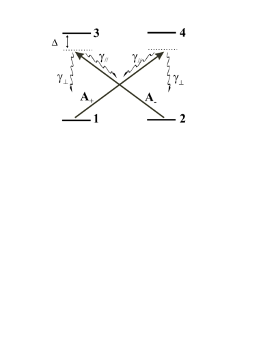
Figure 1: X-like 4-level configuration.

The system considered in this paper is a set of N 4-level cold atoms interacting in an optical cavity driven by a linearly polarized field as represented in Fig 1. We denote $A_{\pm}$ the slowly-varying envelope operators associated with the $\sigma_{\pm}$ components of the light [14]. They are defined from the standard linear polarization components

$$A_{+}=-\frac{A_{x}-iA_{y}}{\sqrt{2}}\;\;,\;\;\;A_{-}=\frac{A_{x}+iA_{y}}{\sqrt{2}}$$ (1)

The atomic frequencies are both equal to $\omega_{at}=\omega_{13}=\omega_{24}$. The field frequency is $\omega$ and the detunings from atomic resonance are equal on both transitions to $\Delta=\omega_{at}-\omega$. The 4-level system is described using collective operators for the N atoms of the ensemble, the optical dipoles being defined in the rotating frame associated to the laser frequency (e.g. $\sigma_{14}=\sum\limits_{i=1}^{N}e^{i\omega t}|1\rangle_{i}\langle 4|_{i}$). The coupling constant between the atoms and the field is defined by $g=\mathcal{E}_{0}d/\hbar$, where $d$ is the atomic dipole and $\mathcal{E}_{0}=\sqrt{\hbar\omega/2\epsilon_{0}\mathcal{S}c}$. With this definition, the mean square value of the field is expressed in number of photons per second. As in Fig 1, the population of level 3 decays with rate $2\gamma_{\perp}$ on level 1 and with rate $2\gamma_{//}$ on level 2, the dipole decay rate being $\gamma=\gamma_{//}+\gamma_{\perp}$. We consider the case of saturated optical pumping and neglect the relaxation rate of the ground states populations. This approximation is well verified for alkali cold atoms [15]. With these conventions, the atom-field hamiltonian is

$$H=\hbar g[A_{+}\sigma_{41}+A_{+}^{\dagger}\sigma_{14}+A_{-}\sigma_{32}+A_{-}^{\dagger}\sigma_{23}]$$ (2)

The atomic evolution is then governed by a set of quantum Heisenberg-Langevin equations

$$\frac{d\sigma_{14}}{dt} = -(\gamma+i\Delta)\sigma_{14}-igA_{+}(\sigma_{11}-\sigma_{44})+F_{14}$$ (3)

$$\frac{d\sigma_{23}}{dt} = -(\gamma+i\Delta)\sigma_{23}-igA_{-}(\sigma_{22}-\sigma_{33})+F_{23}$$ (4)

$$\frac{d\sigma_{11}}{dt} = 2\gamma_{\perp}\sigma_{33}+2\gamma_{//}\sigma_{44}-ig(A_{+}^{\dagger}\sigma_{14}-A_{+}\sigma_{41})+F_{11}$$ (5)

$$\frac{d\sigma_{22}}{dt} = 2\gamma_{//}\sigma_{33}+2\gamma_{\perp}\sigma_{44}-ig(A_{-}^{\dagger}\sigma_{23}-A_{-}\sigma_{32})+F_{22}$$ (6)

$$\frac{d\sigma_{33}}{dt} = -2\gamma\sigma_{33}+ig(A_{-}^{\dagger}\sigma_{23}-A_{-}\sigma_{32})+F_{33}$$ (7)

$$\frac{d\sigma_{44}}{dt} = -2\gamma\sigma_{44}+ig(A_{+}^{\dagger}\sigma_{14}-A_{+}\sigma_{41})+F_{44}$$ (8)

Note that we have not reproduced all the atomic equations, but only those of interest for the following. The Langevin operators $F_{\mu\nu}$ are $\delta$-correlated and their correlation functions are calculated via the quantum regression theorem [16]. We consider a ring cavity with $T$ the transmission of the cavity coupling mirror, $\omega_{c}$ the cavity resonance frequency closest to $\omega$ and $\tau$ the cavity round-trip time. The cavity dephasing is $\Phi_{c}=(\omega-\omega_{c})\tau$. The incoming quantum fields are $A_{\pm}^{in}$ and the field equations read

$$\tau\frac{dA_{+}}{dt} = -(T/2+i\Phi_{c})A_{+}-ig\sigma_{14}+\sqrt{T}A_{+}^{in}$$ (9)

$$\tau\frac{dA_{-}}{dt} = -(T/2+i\Phi_{c})A_{-}-ig\sigma_{23}+\sqrt{T}A_{-}^{in}$$ (10)

3 Steady-state

3.1 Atomic steady state

The atomic steady state is readily obtained by setting the time derivatives to zero and using the fact that a Langevin operator mean value is zero. Defining saturation parameters $s_{\pm}$ for both polarizations,

$$s_{\pm}=\frac{2g^{2}|\langle A_{\pm}\rangle|^{2}}{\Delta^{2}+\gamma^{2}}=\frac{\Omega_{\pm}^{2}/2}{\Delta^{2}+\gamma^{2}},$$ (11)

the atomic steady state is given by

$$\langle\sigma_{14}\rangle=\frac{-igN\langle A_{+}\rangle}{\gamma+i\Delta}\frac{s_{-}}{s_{+}+s_{-}}\frac{1}{1+S}\;,\langle\sigma_{23}\rangle=\frac{-igN\langle A_{-}\rangle}{\gamma+i\Delta}\frac{s_{+}}{s_{+}+s_{-}}\frac{1}{1+S}$$ (12)

$$\langle\sigma_{11}\rangle=N\frac{s_{-}}{s_{+}+s_{-}}\frac{1+s_{+}/2}{1+S}\;\;\;\;\;\;\;\;\;\;,\langle\sigma_{22}\rangle=N\frac{s_{+}}{s_{+}+s_{-}}\frac{1+s_{-}/2}{1+S}$$ (13)

$$\langle\sigma_{33}\rangle=\langle\sigma_{44}\rangle=\frac{N}{4}\frac{S}{1+S}\;\;\;with:\;\;\;S=\frac{2s_{+}s_{-}}{s_{+}+s_{-}}$$ (14)

$\Omega_{\pm}$ are the Rabi frequencies and $S$ is the coupling saturation parameter which plays a symmetrical role with respect to both polarization components. For an x-polarized field, $S=s_{+}=s_{-}=s_{x}/2$ is directly related to the intracavity field intensity.

3.2 Polarization switching

It is well known that such a coupled system may exhibit polarization switching when driven by a linearly polarized field [17, 18]. In fact, the intracavity field intensities depend on the atomic dephasings $\Phi_{\pm}$ and absorptions $a_{\pm}$

$$\Phi_{\pm}=2\Phi_{0}\frac{s_{\mp}}{s_{+}+s_{-}}\frac{1}{1+S} \;\;,\;\; a_{\pm}=2a_{0}\frac{s_{\mp}}{s_{+}+s_{-}}\frac{1}{1+S}$$ (15)

$$\Phi_{0}=\frac{Ng^{2}\Delta}{2(\Delta^{2}+\gamma^{2})} \;\;,\;\; a_{0}=\frac{Ng^{2}\gamma}{2(\Delta^{2}+\gamma^{2})}$$ (16)

with $\Phi_{0}$ and $a_{0}$ the linear dephasing and absorption in the absence of saturation. These quantities depend in turn on the intensities to yield a complex coupled system. In order to derive analytical criteria for polarization switching, we follow the method given in [18] and decompose dephasings and losses into their linear and non-linear parts,

$$\Phi_{\pm}=\Phi_{l}\pm\Phi_{SR}\;\;\; with\;\;\; \Phi_{l}=\frac{\Phi_{0}}{1+S}\;,\;\;\Phi_{SR}=\Phi_{l}x_{SR}$$ (17)

$$a_{\pm}=a_{l}\pm a_{SR}\;\;\; with\;\;\; a_{l}=\frac{a_{0}}{1+S}\;,\;\;a_{SR}=a_{l}x_{SR}$$ (18)

where $\Phi_{SR}$ and $a_{SR}$ are the non-linear circular birefringence and dichroism, related to the ellipticity $\epsilon$ [19]

$$x_{SR}=\frac{s_{-}-s_{+}}{s_{+}+s_{-}}=-\sin 2\epsilon$$ (19)

Thus, as pointed out in the literature [20, 21], the optical pumping induces non-linear self-rotation (SR) of elliptically polarized light. It will be shown in the next section that this effect is responsible for PS in a cavity configuration. Let us first focus on the solution for the $\sigma_{\pm}$ components. Normalizing all the dephasings and absorptions by $T/2$ ($\delta_{j}=2\Phi_{j}/T$ and $\alpha_{j}=2a_{j}/T$), Eqs (9),(10) read in steady state

$$s_{\pm}=\frac{s_{max}}{(1+\alpha_{l}\pm\alpha_{SR})^{2}+(\delta_{l}\pm\delta_{SR}-\delta_{c})^{2}}$$ (20)

with $s_{max}=2/Ts_{x}^{in}$ the maximal intracavity intensity in the absence of absorption. Replacing (20) in (19), we derive the equation for $x_{SR}$: non zero solutions correspond to elliptically polarized states. After straightforward calculations, we obtain

$$x_{SR}=0\;\;\;\; or\;\;\;\; (\alpha_{l}^{2}+\delta_{l}^{2})x_{SR}^{2}=\delta_{l}^{2}+\alpha_{l}^{2}-\delta_{c}^{2}-1$$ (21)

The first trivial solution corresponds to the linearly polarized field. It follows from the second equation and (17),(18) that elliptically polarized states may exist as soon as the existence criterion $C_{ex}$ is satisfied

$$C_{ex}=\frac{\delta_{0}^{2}+\alpha_{0}^{2}}{(1+S)^{2}}-\delta_{c}^{2}-1\geq 0\;\;\;\;\;\;(s_{+}\neq s_{-})$$ (22)

Note that the absorption brings a positive contribution to the existence of asymmetrical solutions: this is due to the fact that non-linear circular dichroism produces ”self-elliptization” of the field. However, this criterion gives no information on the stability of the solutions. In order to get some physical insight into this complicated problem it is useful to look at the evolution of the linearly polarized solution.

3.3 Interpretation of polarization switching

In this section, we give a simple interpretation of PS as the threshold for laser oscillations. Let us consider the linearly polarized solution along the x axis. The adiabatic elimination of the atomic variables leads to

$$\frac{1}{\kappa}\frac{dA_{y}}{dt}=-(1+i\delta_{c})A_{y}+(i\delta_{l}-\alpha_{l})A_{y}-(\delta_{SR}+i\alpha_{SR})A_{x}+\frac{2}{\sqrt{T}}A_{y}^{in}$$ (23)

where $\kappa=T/2\tau$ is the intracavity field decay rate. In (23) all terms have zero mean value and are of order 1 in fluctuations ($\langle A_{x}\rangle\neq 0$). Using $x_{SR}A_{x}=i(A_{y}-A_{x}^{2}/|A_{x}|^{2}A_{y}^{\dagger})$, one obtains

$$\frac{1}{\kappa}\frac{dA_{y}}{dt}=-(1+i\delta_{c})A_{y}+(i\delta_{l}-\alpha_{l})\frac{A_{x}^{2}}{|A_{x}|^{2}}A_{y}^{\dagger}+\frac{2}{\sqrt{T}}A_{y}^{in}$$ (24)

Owing to SR the fluctuations of the orthogonal mode undergo a phase dependent gain. A similar equation has already been derived in previous theoretical works in a single pass scheme [8]. In our configuration the presence of the cavity will lead to oscillations of this mode as soon as the phase sensitive gain is larger than the losses. This condition may be expressed as follows

$$C_{PS}=\frac{\delta_{0}^{2}+\alpha_{0}^{2}}{(1+s_{x}/2)^{2}}-\delta_{c}^{2}-1\geq 0$$ (25)

Obviously, the linearly polarized solution is not stable when $C_{PS}\geq 0$. However, the adiabatical elimination of the atomic variables does not a priori take all causes for instability into account. Yet, we checked that this threshold analysis was consistent with a numerical calculation of the atom-field stability matrix. In the following we use $C_{PS}$ as a stability criterion for the linearly polarized solution. Nevertheless, it does not yield information on the stability of the elliptically polarized solutions, which has been evaluated numerically.
Besides, the ability of a system to produce squeezing being closely related to its static properties, the fluctuations of the vacuum field are expected to be strongly modified in the vicinity of the PS threshold. Since Eq (24) is similar to that of a degenerate optical parametric oscillator (OPO) below the threshold [22], perfect squeezing could be obtained via SR. However, the atomic noise is not included in (24) and is to be carefully evaluated.

3.4 Optical pumping regime

Figure 2: Resonance curves in the optical pumping regime. The parameters are $\delta_{0}=5$, $s_{max}=0.01$. The cavity dephasing corresponding to PS is $\delta_{PS}=4.85$, close to $\delta_{0}$ as given by the PS criterion. When the cavity detuning is scanned from the right, the linear solution is stable until $\delta_{c}=\delta_{PS}$ and unstable afterwards. Then the elliptically polarized solutions, $s_{+}$ and $s_{-}$, become stable for $|\delta_{c}|\leq\delta_{PS}$. We plot also the resonance peaks (dashed line) for the cavity with $0$ or $N$ atoms, in the absence of SR phenomenon.

PS is caused by a competition between the two $\sigma_{\pm}$ optical pumping processes. We can understand the main features of this effect by restraining ourselves to the case where absorption and saturation are negligible: $\Delta\gg\gamma$ and $s_{x}\ll 1$. Neglecting the excited state populations, the optical pumping equations for the ground state populations are

$$\left(\frac{d\sigma_{11}}{dt}\right)_{pumping}=-\gamma_{\perp}s_{+}\sigma_{11}+\gamma_{\perp}s_{-}\sigma_{22}$$ (26)

$$\left(\frac{d\sigma_{22}}{dt}\right)_{pumping}=-\gamma_{\perp}s_{-}\sigma_{22}+\gamma_{\perp}s_{+}\sigma_{11}$$ (27)

so that the $\sigma_{+}$ component tends to pump the atoms into level 2, the $\sigma_{-}$ into 1, and, in steady state, $\sigma_{11}\propto s_{-}$ and $\sigma_{22}\propto s_{+}$. The circular birefringence $\delta_{SR}$ is proportional to the ground state population difference, and consequently, to the intensity difference $s_{+}-s_{-}$ [see (19)]. This simple analysis allows for relating self-rotation to competitive optical pumping and will help us interpret the resonance curves.
Under the previous conditions both criteria (22) and (25) are equivalent and it follows that the linearly polarized solution bifurcates into an elliptically polarized state for $|\delta_{c}|\leq\delta_{PS}=\sqrt{\delta_{0}^{2}-1}$. Consequently, PS is observed as soon as the linear dephasing is greater than half the cavity bandwidth ($\delta_{0}\geq 1$). This represents an easily accessible condition from an experimental point of view : in our cesium experiment using a magneto-optical trap [9, 10], the number of atoms interacting with the light is $N\simeq 7\;10^{6}$. To find realistic experimental parameters, we assimilate each one of our X-model transitions to the transition $6S_{1/2}\;(F=4)-6P_{3/2}\;(F=5)$ of the $D_{2}$ line of ${}^{133}Cs$, for which $\gamma/2\pi=2.6$ MHz. The square of the coupling constant $g$ is proportional to the ratio of the diffusion section at resonance to the transversal surface $S=0.1$ mm² of the beam, $g^{2}=3\gamma\lambda^{2}/4\pi S=4.24$ Hz. The cavity transmission is 10%. To obtain a sufficiently high non-linearity, keeping the absorption low, a good detuning is $\Delta\simeq 20\gamma$, so that an approximate value for the linear detuning is $\delta_{0}\simeq 5$. Note that the saturation parameters of (11) are simply

$$s_{\pm}=\frac{\gamma^{2}}{\gamma^{2}+\Delta^{2}}\frac{I_{\pm}}{I_{sat}}$$ (28)

The saturation intensity being $I_{sat}=\epsilon_{0}c\gamma^{2}\hbar^{2}/d^{2}=1.05$ mW/cm² [9], typical values for $s_{\pm}$ are 0.1-1.

In Fig 2 are represented the admissible intensities for the $\sigma_{+}$ and $\sigma_{-}$ components versus the cavity detuning for typical experimental values of the parameters. The peak centered on $\delta_{c}=\delta_{0}$ corresponds to the symmetrical solution. When the cavity is scanned from right to left, the linearly polarized field ($s_{+}=s_{-}$) intensity increases until the PS threshold is reached ($\delta_{c}=\delta_{PS}\simeq\delta_{0}$). Then one elliptically polarized state becomes stable. The predominant circular component, say $\sigma_{+}$, creates, via the optical pumping process (26-27), a positive orientation of the medium $\sigma_{11}\simeq 0$, $\sigma_{22}\simeq N$. Since the atomic dephasing decreases to zero for the $\sigma_{+}$ component ($\delta_{+}\simeq 0$), as if it were propagating in an empty cavity. Hence, the solution draws close to the zero-dephasing peak, that is, close to resonance in the range $|\delta_{c}|\leq\delta_{PS}$. On the other hand the $\sigma_{-}$ component ”sees” all the atoms ($\delta_{-}\simeq 2\delta_{0}$) and breaks down to fit the peak centered on $\delta_{c}=2\delta_{0}$, which is far from resonance. In order to illustrate this interpretation of the resonance curves, the two Airy peaks centered on $\delta_{c}=0$ and $\delta_{c}=2\delta_{0}$ are represented in Fig 2. As the cavity detuning is decreased both asymmetrical solutions reunite when the criterion (25) is no longer satisfied and the linear solution becomes stable again. These simple interpretations will help us understand the much more complex general case, when absorption and saturation come into play.
As discussed in Ref [18], taking into account the ground state relaxation rate $\gamma_{0}$ yields tristability in the unsaturated optical pumping regime ($\gamma_{\perp}s_{\pm}\ll\gamma_{0}$). We will now show that the optical saturation also leads to tristability.

3.5 Tristability

It is well-known that saturation may induce multistability for the linearly polarized field [23] in our configuration and substantially modify the steady state. When the non-linearity is sufficient, there may be three possible values for the x-polarized field intensity. Therefore, saturation is an additional cause of instability for the symmetrical solution. In Fig LABEL:fig3, we plotted the same curves as in Fig 2, but for higher values of $s_{max}$ and $\delta_{0}$. As expected, the linearly polarized state solution is distorted as a consequence of the non-linear effect. The effect of absorption is also clear: whereas the symmetrical peak height is reduced, the $\sigma_{+}$ dominant peak height is not. Indeed, the $\sigma_{+}$ component ”sees” no atoms after the switching.
Besides, the system now exhibits tristability for a certain range of the cavity detuning. As mentioned previously the existence of asymmetrical solutions is related to the positivity of $C_{ex}$, whereas the stability of the symmetrical solution is given by $C_{PS}$. For instance, on Fig LABEL:fig3, $C_{ex}=0$ for $\delta_{c}=\delta_{ex}=5.6$ and the threshold $C_{PS}=0$ is reached for a dephasing $\delta_{c}=\delta_{PS}=2.6$. Thus, in the range $\delta_{PS}\leq\delta_{c}\leq\delta_{ex}$, two different sets of asymmetrical solutions exist, in addition to the linear polarization state. This phenomenon is due to the saturation experienced by the $\sigma_{+}$ and $\sigma_{-}$ components. As expected, we checked that only the lower branch of each asymmetrical curve is stable, leading to tristability for the polarization state : linear, $\sigma_{+}$-dominant or $\sigma_{-}$-dominant. The system switches for a different value of the cavity detuning if the cavity is scanned from left to right, or from right to left (see Fig LABEL:fig3). Hence, unlike the unsaturated case, saturation induces a multistable behavior and a hysteresis cycle now appears in the resonance curve.

This brief study of the resonance curve for typical parameters leads to an essential observation: the lower branch of the bistability curve for the linear polarized field is not stable. We may wonder if there is a domain of the parameter space for which it is not the case. Since the quantum fluctuations are expected to be most reduced in the vicinity of the lower turning point [24, 25], the answer is of crucial importance for squeezing and will be treated in the next section.

3.6 Competition between SR and saturation

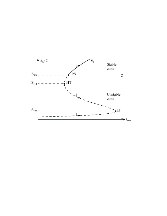
Figure 4: Bistability curve: linearly polarized field intensity $S=s_{x}/2$ as a function of $s_{max}$. PS is the switching threshold, $HT$ and $LT$ the higher and lower turning points. For certain incident intensities $s_{max}$ three solutions (1,2,3) exist for the intracavity intensity $s_{x}/2$, of which only one (3) is stable, instead of the usual two (1,3) in the absence of PS phenomenon.

To complete the analysis of the steady state, we would like to emphasize that, when the cavity is scanned, PS always happens before reaching the higher turning point of the bistability curve. In order to get some insight into this complicated problem, it is worth looking at Fig 4. We plotted the typical S-shaped variation of the linearly polarized field intensity $s_{x}$ versus the incoming intensity $s_{max}$, for a fixed value of the cavity detuning $\delta_{c}$. We choose the parameters so that there is bistability for this state of polarization and report the position of the lower ($LT$) and the higher ($HT$) turning points. In the absence of the PS phenomenon, the solutions between $HT$ and $LT$ are unstable (like 2 on Fig 4), whereas solutions on the lower (1) and higher (3) branches are stable. However the stability of the linear polarization is modified by the PS effects. To a fixed value of the dephasing corresponds the PS intensity $S_{PS}$ cancelling $C_{PS}$ in (25); if $S=s_{x}/2\leq S_{PS}(\delta_{c})$, then the linear polarization is unstable. Hence, if $S_{PS}(\delta_{c})\geq S_{HT}$ is satisfied in the whole parameter space, then PS occurs before reaching $HT$, and, consequently, the lower branch is never stable.
This general feature is shown on Fig 5, in which we represented different bistability curves as in Fig 4. The upper branch of AB is the $HT$ curve (the ensemble of the higher turning points when $\delta_{c}$ is varied), the lower branch is the $LT$ curve. The dashed curve shows the ensemble of the intensities $S_{PS}$ for which the polarization switches. This curve is always above the $HT$ curve, confirming that the linear polarization always becomes unstable on account of PS first. What is more, we see that PS is closer to $HT$ for low values of $s_{x}$. We thus expect this situation to be the most favorable to achieve squeezing via optical bistability. We checked that varying the parameters $\delta_{0}$ and $\Delta$ does not change the conclusion.

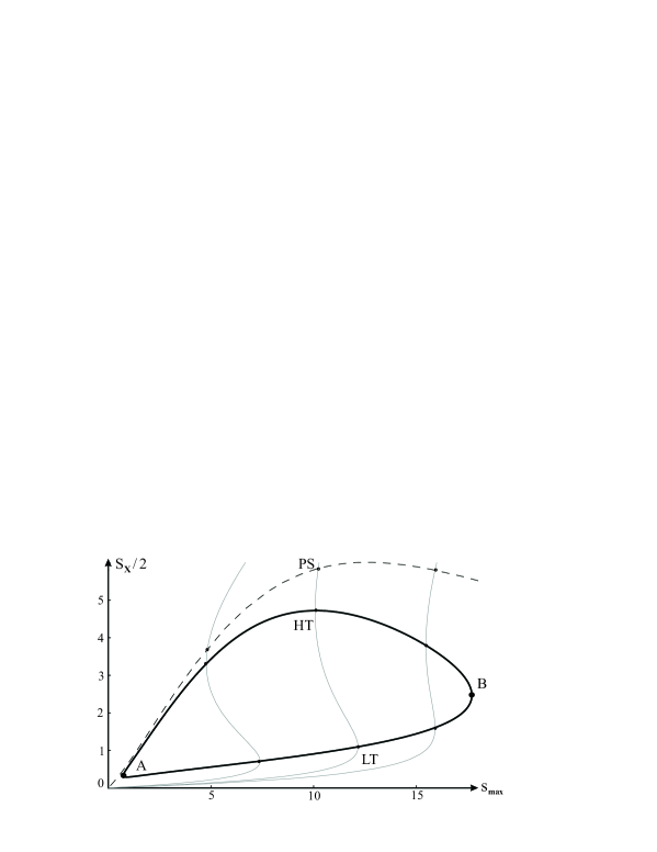
Figure 5: Bistability curves $S=s_{x}/2$ as a function of $s_{max}$ for field $A_{x}$. The three S-shaped curves correspond to different values of the cavity dephasing ($\delta_{c}=-0.25,0.3,1.1$ from left to right), $\delta_{0}$ and $\Delta$ having the same value as in Fig LABEL:fig3. The AB segments represent the $HT$ (higher) and $LT$ (lower) curves. The dashed curve is the ensemble of the intensities $S_{PS}$ for which polarization switching occurs. The system exhibits bistability for $s_{A}\leq s_{max}\leq s_{B}$.

To conclude this section, we would like to point out that bistability, as well as PS, may disappear when the saturation is too high, as can be seen from Fig 4. However, we will focus on the low saturation case in the large detuning limit which is the most favorable case for squeezing, and provides analytical results, as well as a clear physical understanding.

4 Mean field fluctuations

Since we are interested in the quantum fluctuations, we linearize the quantum operators around their steady state values following the standard linear input-output method [24]. The elliptically polarized solutions are not of great interest for squeezing since the predominant circular component sees no atom and the other has negligible intensity. Therefore, in all the following, we focus on the linearly polarized state and study how both the mean field $A_{x}$ and the orthogonal vacuum field $A_{y}$ may be squeezed. We have calculated the outgoing fields noise spectra via a full quantum treatment (see e.g. [25]) involving the four-level system. The outgoing fields are standardly defined from the input-output relation [24]:

$$A_{x,\;y}^{out}=\sqrt{T}A_{x,\;y}-A_{x,\;y}^{in}$$ (29)

Yet, to provide clear interpretations as well as analytical results, we derive simplified equations, first for the mean field mode $A_{x}$, then for the vacuum mode $A_{y}$.
A similar equation to (23) can be derived for the field $A_{x}$ with a term arising from SR in $\delta_{SR}A_{y}$. In the linearization, this product of zero mean value operators vanishes, so that we only have to take saturation into account to derive the spectra of $A_{x}$. Field squeezing owing to optical bistability has been widely studied [25, 26, 27] and is known to occur on a frequency range given by the cavity bandwidth $\kappa$. The most favorable configuration is the bad cavity limit: $\kappa$ is greater than $\gamma$ (in our experiment, $\kappa\simeq 2\gamma$). In the large detuning limit, $\Delta\gg g|A_{x}|\gg\gamma$, the equation for $A_{x}$ reads at order 3 in $\gamma/\Delta$,

$$\frac{1}{\kappa}\frac{d}{dt}\delta A_{x}=-(1+i\delta_{c}-i\delta_{0})\delta A_{x}+i\delta_{0}\frac{s_{x}}{2}\left[2\delta A_{x}+\frac{A_{x}^{2}}{|A_{x}|^{2}}\delta A_{x}^{\dagger}\right]+\frac{2}{\sqrt{T}}A_{x}^{in}$$ (30)

where $A_{x}$ is short for $\langle A_{x}\rangle$. This simplified equation yields the classical Kerr terms in $A_{x}^{2}\delta A_{x}^{\dagger}$ producing squeezing. Note that absorption, dispersion and the associated atomic noise are not included in (30). The spectra taking absorption and dispersion into account can be easily derived and are shown on Fig 7. The associated susceptibility and correlation matrices, $[\chi]_{Kerr}$ and $[\sigma]_{Kerr}$, of the linear input-output theory are reproduced in Appendix, and the comparison with a Kerr medium is discussed in [25]. The situation is more complex for the orthogonal mode on account of SR.

5 Vacuum fluctuations

As mentioned in Sec 3.3, SR seems to be a very promising candidate for generating vacuum squeezing. However, a careful analysis of the atomic noise, which cannot be neglected, is necessary in the squeezing calculations. In the optical pumping regime the circular birefringence, $\delta_{SR}=-2\delta_{0}J_{z}/N$, is proportional to the ground state population difference $J_{z}=(\sigma_{22}-\sigma_{11})/2$ (see Sec 3.4). The SR effect is thus closely related to the fluctuations of $J_{z}$, and consequently to the fluctuations of $A_{y}$ via the coupling term in $A_{x}\delta_{SR}$ [Eq (23)]. Therefore, we derive general equations for $\delta A_{y}$ and $\delta J_{z}$ in the Fourier domain, and examine their low and high frequency limits. For the sake of simplicity, absorption and linear dispersion, again, are not shown; however, the additional terms are included in the Appendix. As previously we place ourselves in the large detuning limit with $s_{x}\ll 1$ and obtain, discarding terms of order greater than $(\gamma/\Delta)^{3}$,

$$-i(\omega/\kappa)\delta A_{y} = -(1+i\delta_{c}-i\delta_{0})\delta A_{y}-i\delta_{0}\frac{s_{x}}{4}\left[3\delta A_{y}-\frac{A_{x}^{2}}{|A_{x}|^{2}}\delta A_{y}^{\dagger}\right]$$ (31)

$$+\beta(\omega)\frac{2\delta_{0}}{N}A_{x}\delta J_{z}+\frac{2}{\sqrt{T}}\delta A_{y}^{in}+F_{A_{y}}$$

$$-i\omega\delta J_{z} = -\gamma_{p}\alpha(\omega)\left[\delta J_{z}-\lambda(\omega)\left(1-\frac{s_{x}}{2}\right)\frac{N}{2}\frac{\delta S_{z}}{|A_{x}|^{2}}\right]+F_{z}$$ (32)

where $S_{z}=i(A_{x}A_{y}^{\dagger}-A_{x}^{*}A_{y})$ is the usual Stokes parameter (see Sec 6) and

$$\alpha(\omega)=\left[1-\frac{i\omega}{4\gamma_{\perp}}\right]\frac{\beta(\omega)}{\lambda(\omega)}\;\;,\;\;\;\beta(\omega)=1-\frac{s_{x}}{4\lambda(\omega)}\;\;,\;\;\;\lambda(\omega)=\frac{2\gamma-i\omega}{2(\gamma-i\omega)}$$ (33)

with $F_{A_{y}}$ and $F_{z}$ the Langevin operators associated to $A_{y}$ and $J_{z}$ after the adiabatical eliminations, $\gamma_{p}=\gamma_{\perp}s_{x}$ the optical pumping rate. In (31), the last term of the first line is a crossed Kerr term and clearly contributes to squeezing. We also see that the coupling with $J_{z}$ is strongly frequency-dependant and requires a careful investigation. In the next sections, we discuss the low and high frequency limits to further simplify the previous equations and give simple interpretations for the squeezing.

5.1 Low frequency: SR effect

Again, to stress the effects on the fluctuations only due to SR, we neglect the terms in $s_{x}$ responsible for the Kerr effect, which will be studied in the next section, and place ourselves in the optical pumping regime, keeping only terms of order 1 in $\gamma/\Delta$. Note that this approximation consists in adiabatically eliminating the optical dipoles and neglecting the excited state populations and thus limits the analysis to the range of frequencies $\omega\ll\gamma,\gamma_{\perp}$. Under these conditions, one has $\alpha(\omega)\simeq 1$, $\beta(\omega)\simeq 1$, $\lambda(\omega)\simeq 1$ and Eq (32) reduces to the linearized optical pumping equation

$$-i\omega\delta J_{z}=-\gamma_{p}\left[\delta J_{z}-\frac{N}{2}\frac{\delta S_{z}}{|A_{x}|^{2}}\right]+F_{z}$$ (34)

It is clear that the fluctuations of $J_{z}$ are governed by the time constant $\gamma_{p}$, consistently with the optical pumping approximation $\gamma_{p}\ll\gamma$. SR is effective only at low frequency. Plugging (34) back into (31), one gets

$$(1+i\delta_{c}-i\omega/\kappa)\delta A_{y} = i\delta_{0}\left[1-\frac{\gamma_{p}}{\gamma_{p}-i\omega}\right]\delta A_{y}$$ (35)

$$+i\delta_{0}\frac{\gamma_{p}}{\gamma_{p}-i\omega}\frac{A_{x}^{2}}{|A_{x}|^{2}}\delta A_{y}^{\dagger}+\frac{2}{\sqrt{T}}\delta A_{y}^{in}+\tilde{F}_{A_{y}}$$

The SR term comes with an amplitude $\delta_{0}$ ($\propto\gamma/\Delta$) around zero frequency, which is much greater than the usual third order saturation non-linearity. Very good squeezing could be expected if it were not for the noise coming from the atoms $\tilde{F}_{A_{y}}$, which we now study. The fluctuation operator arising from atomic and field fluctuations reads

$$\tilde{F}_{A_{y}}=\frac{2\delta_{0}A_{x}}{N}\frac{F_{z}}{\gamma_{p}-i\omega}+F_{A_{y}}$$ (36)

The second term $F_{A_{y}}$ is responsible for the noise due to absorption. The first term includes the optical pumping noise. One calculates the correlation function of $F_{z}$ via the quantum regression theorem [16]

$$\langle F_{z}(\omega)F_{z}(\omega^{\prime})\rangle=2\pi\delta(\omega+\omega^{\prime})N\gamma_{p}/2$$ (37)

so that

$$\langle\tilde{F}_{A_{y}}(\omega)\tilde{F}_{A_{y}}^{\dagger}(\omega^{\prime})\rangle \simeq \frac{4\delta_{0}^{2}A_{x}^{2}}{N^{2}}\frac{1}{\gamma_{p}^{2}+\omega^{2}}\langle F_{z}(\omega)F_{z}(\omega^{\prime})\rangle$$ (38)

$$= 2\pi\delta(\omega+\omega^{\prime})\frac{C}{4}\frac{\gamma}{\gamma_{\perp}}\frac{\gamma_{p}^{2}}{\gamma_{p}^{2}+\omega^{2}}$$ (39)

in which we introduced $C=g^{2}N/T\gamma$ the cooperativity parameter quantifying the strength of the atom-field coupling via the cavity ($C\sim 100$ in our Cs experiment). For $\omega\ll\gamma_{p}$ the noise is thus much more important than the losses due to absorption and therefore has a dramatic influence on the squeezing that could have been produced by the SR term. Following the method given in [25], we derive the susceptibility and correlation matrices which are given in Appendix. We can then calculate the outgoing vacuum field spectrum for all the quadratures. Minimal and maximal spectra are plotted on Fig LABEL:fig6 in the ”close-to-bad” cavity limit ($\kappa=2\gamma$) corresponding to our experimental configuration. Whereas the first is close to the shot-noise level, the second is extremely noisy. In the good cavity limit, the noise is even more important. The conclusion is that the optical pumping process adds too much noise at zero frequency for SR to generate vacuum squeezing. However, this low frequency noise does not prevent squeezing at higher frequencies.

5.2 High frequency limit: crossed Kerr effect

If one repeats the previous calculation keeping the first order saturation terms in $s_{x}$ and considers frequencies $\omega\gg\gamma$, one finds

$$\delta J_{z}(\omega)=\frac{N}{2}\frac{s_{x}}{4}\frac{\delta S_{z}(\omega)}{|A_{x}|^{2}}$$ (40)

This is not surprising, since the evolution times considered are small with respect to the atomic relaxation time. The system behaves as if $\sigma_{+}$ and $\sigma_{-}$ were independent. In fact, let us consider two independent two-level systems, 1-4 and 2-3, each with $N/2$ atoms. In the large detuning limit, one has $\sigma_{44}=\sigma_{11}s_{+}/2$ and $\sigma_{33}=\sigma_{22}s_{-}/2$, and the atomic fluctuations follow the field fluctuations [25] (still at order 3 in $(\gamma/\Delta)$)

$$\delta\sigma_{11}(\omega)=-\delta\sigma_{44}(\omega)=-\frac{N}{2}\frac{\delta s_{+}}{2}\;\;,\;\;\;\delta\sigma_{22}(\omega)=-\delta\sigma_{33}(\omega)=-\frac{N}{2}\frac{\delta s_{-}}{2}$$ (41)

so that, using $|A_{x}|^{2}\delta(s_{+}-s_{-})=s_{x}\delta S_{z}$, we retrieve (40). This equation shows that the fluctuations of $J_{z}$ are only caused by saturation and their contribution adds to the crossed Kerr terms already mentioned in (31) to retrieve a similar ”Kerr” equation for $A_{y}$ to that of $A_{x}$ at high frequency

$$-i(\omega/\kappa)\delta A_{y} = -(1+i\delta_{c}-i\delta_{0})\delta A_{y}$$ (42)

$$-i\delta_{0}\frac{s_{x}}{2}\left[2\delta A_{y}-\frac{A_{x}^{2}}{|A_{x}|^{2}}\delta A^{\dagger}_{y}\right]+\frac{2}{\sqrt{T}}\delta A_{y}^{in}+F_{A_{y}}$$

This high frequency behavior is thus characterized by the same Kerr-induced optimal squeezing on both polarization modes, consistently with the previous analysis for two independent two-level systems. More precisely, the optimal squeezing spectra are the same for each mode, but involve orthogonal quadratures [because of the sign difference in the Kerr terms between (30) and (42)]. We now plot the outgoing fields $A_{x,\;y}^{out}$ squeezing spectra and discuss the squeezing optimization.

5.3 Squeezing spectra

To derive spectra for the whole frequency range, we combine both effects by adding the matrices obtained in the two asymptotical regimes studied previously. We write the complete susceptibility and correlation matrix under the form $[\chi(\omega)]_{y}=[\chi(\omega)]_{Kerr}+[\chi(\omega)]_{SR}$ and $[\sigma(\omega)]_{y}=[\sigma(\omega)]_{Kerr}+[\sigma(\omega)]_{SR}$, where the Kerr matrices are those obtained in the high frequency limit, and the SR matrices those obtained at low frequency (see Appendix for analytical expressions). This approximation is good since Kerr effect is negligible at low frequency compared to SR, while SR breaks down at high frequency.
In Fig 7, typical spectra for a working point close to the PS threshold are represented. The parameters are chosen to be as close to the experimental situation as possible [11]. We compared these approximate spectra (a) with those obtained with a full 4-level calculations based on the linear input-output theory (b). The analytical spectra combining Kerr and SR effects show indeed an excellent agreement with the exact calculations, as long as the saturation is low. As shown previously, the SR spectrum is close to the shot-noise level. The Kerr spectrum is accurate for $A_{y}$ only for $\omega\gg\gamma$ and extends on a range of several $\kappa$ as expected [25]. The combined spectrum (a) confirms that SR destroys completely the squeezing at low frequency and reproduces well the exact behavior (b). The best squeezing for $A_{y}$, obtained at intermediate frequencies, is about 25%.
Note that the Kerr spectrum in (a) is also valid for field $A_{x}$ for all frequencies and 45% of squeezing is obtained at zero frequency. The situation for the mean field $A_{x}$ is identical to that of a circularly polarized field with intensity $s_{x}/2$ interacting with $N/2$ two-level atoms as in [25], for which the Kerr spectrum shows good agreement with the exact spectrum.

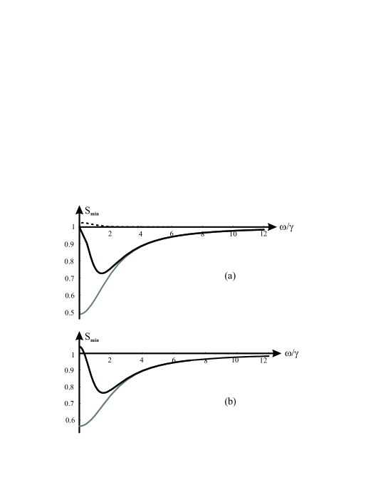
Figure 7: (a) Analytical minimal spectra for $A_{y}^{out}$ given by the SR effect (dashed), by the Kerr effect (light) and by both effects (dark). (b) Exact spectra for the mean field mode $A_{x}^{out}$ (light) and the orthogonal vacuum mode $A_{y}^{out}$ (dark). Parameters values: $\delta_{0}=5$, $\Delta=20\gamma$, $\gamma/\gamma_{\perp}=3$, $\kappa=2\gamma$, $s_{max}=0.1$, $\delta_{c}=4.6$.

As mentioned in Sec 3.6, we expect squeezing to improve in the vicinity of the PS threshold. We verified this behavior by plotting on Fig 8 the evolution of the spectra when the cavity is scanned while keeping the incident intensity ($\propto s_{max}$) constant. It appears clearly that the best squeezing is obtained at the peak of the resonance curve, right before the switching. This is due to the fact that, in the low saturation regime, the PS threshold is close to the point where saturation process is the most efficient.

Figure 8: Minimal spectra for the vacuum field (plain) and the mean field (dashed) for different working points. $\delta_{0}=5$, $\Delta=20\gamma$, $\kappa=2\gamma=6\gamma_{\perp}$, $s_{max}=0.1$. The working points coordinates are: A ($\delta_{c}=\delta_{SR}=4.6$, $s_{x}/2=0.065$), B ($\delta_{c}=5.78$, $s_{x}/2=0.04$), C ($\delta_{c}=6.79$, $s_{x}/2=0.02$). The inset shows the working points positions on the resonance curve.

We then study the effect of saturation and plot on Fig 9 various spectra corresponding to working points close to PS with increasing saturation. The conclusion is that, for given values of the detuning $\Delta$ and linear dephasing $\delta_{0}$, there is an optimal value of $s_{x}$ for squeezing. This is due to the fact that the range for which SR adds noise increases with the saturation and eventually destroys Kerr-induced squeezing. The optimal saturation value thus corresponds to a compromise between added noise and Kerr squeezing in the intermediate frequency range. Therefore, a bad cavity is preferable ($\kappa\gg\gamma$), since Kerr-induced squeezing occurs on a frequency range given by $\kappa$ and SR destroys squeezing for frequencies smaller than $\gamma$. Spectra for different cavities are represented in Fig 10. The case $\kappa=2\gamma$ corresponds to the experimental situation, ”close-to-bad cavity”, the other curves to increasingly bad cavities. Since SR is effective on a range smaller and smaller compared to the cavity bandwidth, its effect becomes negligible, and 75% of squeezing can be obtained.
The conclusion is that very interesting squeezing values can be reached in the bad cavity limit for both the mean field mode and the orthogonal field mode. In the next section, we establish the link between polarization squeezing and the vacuum squeezing obtained in our system.

Figure 9: Minimal spectra for the vacuum field for different saturation values $s_{max}$. For each value of $s_{max}$, the working point is chosen close to PS. Parameters: $\delta_{0}=5$, $\Delta=20\gamma$, $\kappa=2\gamma=6\gamma_{\perp}$.

Figure 10: Minimal spectra for the vacuum for different $\rho=\kappa/\gamma$ (short dash: $\rho=2$, long dash: $\rho=10$, plain: $\rho=50$). For each value of $\rho$, the saturation is optimized. Parameters: $\delta_{0}=5$, $\Delta=20\gamma$, $\gamma/\gamma_{\perp}=3$.

6 Polarization squeezing

The noise of the mode with orthogonal polarization with respect to the mean field is commonly referred to as polarization noise. However, the study of the polarization state fluctuations requires the introduction of the quantum Stokes operators [12, 13, 28]

$$S_{0}(t)=A^{{\dagger}}_{x}A_{x}+A^{{\dagger}}_{y}A_{y} \hskip 2.84544pt,\hskip 28.45274pt S_{x}(t)=A^{{\dagger}}_{x}A_{x}-A^{{\dagger}}_{y}A_{y}$$ (43)

$$S_{y}(t)=A^{{\dagger}}_{x}A_{y}+A^{{\dagger}}_{y}A_{x} \hskip 2.84544pt,\hskip 28.45274pt S_{z}(t)=i(A^{{\dagger}}_{y}A_{x}-A^{{\dagger}}_{x}A_{y})$$ (44)

To be consistent with the definition of our slowly-varying envelope operators $A_{x}$, $A_{y}$, these Stokes operators are time-dependent and expressed in number of photons per second [14]. They obey the following commutation relationships

$$\left[S_{0}(t),S_{i}(t^{\prime})\right]=0\hskip 19.91684ptand\hskip 19.91684pt\left[S_{i}(t),S_{j}(t^{\prime})\right]=2i\epsilon_{ijk}S_{k}\delta(t-t^{\prime})$$ (45)

with $i,j,k=x,y,z$ and then the spectral noise densities of these operators, defined by $\langle S_{i}(\omega)S_{i}(\omega^{\prime})\rangle=2\pi\delta(\omega+\omega^{\prime})V_{S_{i}}(\omega)$, satisfy uncertainty relations

$$V_{S_{i}}(\omega)V_{S_{j}}(\omega)\geq\epsilon_{ijk}|\langle{S_{k}\rangle}|^{2}$$ (46)

The coherent polarization state correspond to the case where both modes $A_{x}$ and $A_{y}$ are coherent states. Then the noise densities of the Stokes parameters are constant and all equal to $V_{S_{i}}(\omega)=\langle S_{0}\rangle=|\langle A_{x}\rangle|^{2}+|\langle A_{y}\rangle|^{2}$ for $i=0,x,y,z$. The so called polarization squeezing is achieved if one or more of these quantities (except $V_{S_{0}}$) is reduced below the coherent state value

$$\frac{V_{S_{i}}(\omega)}{S_{0}}\leq 1\hskip 42.67912pt(i=x,y,z)$$ (47)

If the mean field is x-polarized, then $\langle S_{0}\rangle=\langle S_{x}\rangle=|\langle A_{x}\rangle|^{2}$ and $\langle S_{y}\rangle=\langle S_{z}\rangle=0$. At first order in noise fluctuations, $\delta S_{y}$ and $\delta S_{z}$ read

$$\delta S_{y} = |\langle A_{x}\rangle|\left(\delta A^{{\dagger}}_{y}e^{i\theta_{x}}+\delta A_{y}e^{-i\theta_{x}}\right)\;=|\langle A_{x}\rangle|\;\delta X_{A_{y}}(\theta_{x})$$ (48)

$$\delta S_{z} = i|\langle A_{x}\rangle|\left(\delta A^{{\dagger}}_{y}e^{i\theta_{x}}-\delta A_{y}e^{-i\theta_{x}}\right)=|\langle A_{x}\rangle|\;\delta X_{A_{y}}(\theta_{x}+\pi/2)$$ (49)

where $\theta_{x}$ is the phase of the mean field and $X_{A_{y}}(\theta)=A^{{\dagger}}_{y}e^{i\theta}+A_{y}e^{-i\theta}$ is the quadrature with angle $\theta$ of the orthogonal mode. Therefore the fluctuations of these two Stokes parameters are proportional to the quadrature noise of $A_{y}$ and the polarization squeezing of $S_{y}$ and $S_{z}$ is simply related to the vacuum squeezing that we have studied in the previous sections. The physical meaning of this result is clear: let us choose $\theta_{x}=0$, then geometric jitter on the polarization is due to the intensity fluctuations of $A_{y}$ ($\propto\delta S_{y}$), whereas the fluctuations of the ellipticity are caused by the phase fluctuations ($\propto\delta S_{z}$). In the general case, the squeezed and antisqueezed Stokes parameters are found to be

$$S_{sq} = \cos(\theta_{x}-\theta_{sq})S_{y}+\sin(\theta_{x}-\theta_{sq})S_{z}$$ (50)

$$S_{antisq} = \sin(\theta_{x}-\theta_{sq})S_{y}-\cos(\theta_{x}-\theta_{sq})S_{z}$$ (51)

Note that, unlike [2, 3, 4, 7], there is no need to lock the phase-shift difference $\theta_{x}-\theta_{sq}$, since it is automatically done in this system; this property appears clearly in Eq (42) where $\langle A_{x}^{2}\rangle/|\langle A_{x}\rangle|^{2}=e^{2i\theta_{x}}$. Since the new set of the Stokes parameters $S_{0}$, $S_{x}$, $S_{sq}$ and $S_{antisq}$ still satisfy the relationships (46), we obtain polarization squeezing in our system as soon as any quadrature of the vacuum field $A_{y}$ is squeezed, and the results of the previous sections can be applied to the squeezed Stokes component.

7 Conclusion

We have presented a study of polarization switching in an X-like 4-level atoms ensemble illuminated by a linearly polarized light in an optical cavity. PS has been traced to self-rotation and simple criteria allow for a clear understanding of the switching effects and the multistable behavior of the system. The steady state analysis enables one to figure out the interesting working points for squeezing.
In terms of squeezing the respective contributions of SR and saturation have been investigated and compared to a full quantum calculation. Since the propensity for squeezing of SR is cancelled by atomic noise at low frequency, the squeezing originates from Kerr effect. The mean field mode is squeezed via the usual saturation effects, whereas the vacuum mode squeezing is induced by the mean field via crossed Kerr effect. Both SR and crossed Kerr effects can be dissociated in a bad cavity configuration, thus allowing for high squeezing values. Last, this vacuum squeezing is shown to be equivalent to squeezing one Stokes operator.

Appendix A

Using the input-output theory notations [24],[25], we give here the expressions of the susceptibility matrix $[\chi(\omega)]$ and the correlation matrix $[\sigma(\omega)]$ for field $A_{y}$. In the high frequency limit, they resume to those derived in [25] in the large detuning limit

$$[\chi(\omega)]_{Kerr}=\frac{1}{2\Delta}\left(\begin{array}[]{cc}1&0\\ 0&1\end{array}\right) +\frac{1}{2\Delta^{2}}\left(\begin{array}[]{cc}i\gamma+\omega&0\\ 0&-i\gamma-\omega\end{array}\right)$$ (56)

$$-\frac{g^{2}}{2\Delta^{3}}\left(\begin{array}[]{cc}2|A_{x}|^{2}&\varepsilon A_{x}^{2}\\ \varepsilon A_{x}^{*2}&2|A_{x}|^{2}\end{array}\right)$$ (59)

$\varepsilon=-1$ yields the susceptibility matrix for the vacuum mode. To retrieve the matrix for $A_{x}$, $\varepsilon$ should be taken equal to $+1$. This matrix corresponds to approximating the atoms ensemble with a Kerr medium: the term of order 1 in $1/\Delta$ is the linear dephasing, the second order matrix represents dispersion and absorption and the third order term is the non-linear dephasing corresponding to the Kerr effect. The associated correlation matrix is

$$[\sigma(\omega)]_{Kerr}=\frac{\gamma}{\Delta^{2}}\left(\begin{array}[]{cc}1&0\\ 0&0\end{array}\right)$$ (60)

In the Kerr limit, the atomic noise comes only from the frequency independent linear losses of the Kerr medium, which acts as a beamsplitter for the field. Similar matrices can be derived for field $A_{x}$ in agreement with (30). At low frequency, however, the previous matrices have to be completed by

$$[\chi(\omega)]_{SR}=-\frac{1}{2\Delta}\frac{\gamma_{p}}{\gamma_{p}-i\omega}\left(\begin{array}[]{cc}1&-A_{x}^{2}/|A_{x}|^{2}\\ -A_{x}^{*2}/|A_{x}|^{2}&1\end{array}\right)$$ (63)

$$[\sigma(\omega)]_{SR} = \frac{\gamma_{p}^{2}}{4\gamma_{\perp}(\gamma_{p}^{2}+\omega^{2})}\left(\begin{array}[]{cc}1&-A_{x}^{2}/|A_{x}|^{2}\\ -A_{x}^{*2}/|A_{x}|^{2}&1\end{array}\right)$$ (69)

$$+\frac{\gamma_{p}}{2\Delta(\gamma_{p}^{2}+\omega^{2})}\left(\begin{array}[]{cc}-2\omega&\omega+i\gamma_{p}\\ \omega-i\gamma_{p}&0\end{array}\right)$$

For $\omega\ll\gamma_{p}$, the vacuum correlation matrix is equivalent to

$$[\sigma(\omega)]_{SR}\sim\frac{\gamma_{p}^{2}}{4\gamma_{\perp}(\gamma_{p}^{2}+\omega^{2})}\left(\begin{array}[]{cc}1&-A_{x}^{2}/|A_{x}|^{2}\\ -A_{x}^{*2}/|A_{x}|^{2}&1\end{array}\right)$$ (70)

so that a lot of noise is reported on all the quadratures of $A_{y}$ for frequencies of the order of $\gamma_{p}$, as pointed out in Sec 5.1. For frequencies $\omega\gg\gamma$, the SR noise terms vanish, allowing for crossed Kerr effect to produce squeezing.

References

- [1] L. Davidovich, Rev. Mod. Phys. 68, 127 (1996), and references therein.
- [2] P. Grangier, R.E. Slusher, B. Yurke, A. LaPorta, Phys. Rev. Lett. 59, 2153 (1987).
- [3] J. Hald, J.L. Sorensen, C. Shori, E.S. Polzik, 83, 1319 (1999).
- [4] W.P. Bowen, R. Schnabel, H.A. Bachor, P.K. Lam, Phys. Rev. Lett. 88, 093601 (2002); W.P. Bowen, N. Treps, R. Schnabel, P.K. Lam, Phys. Rev. Lett. 89, 253601 (2002).
- [5] A.P. Alodjants, A.M. Arakelian, A.S. Chirkin, JEPT 108, 63 (1995); N.V. Korolkova, A.S. Chirkin, J. Mod. Opt. 43, 869 (1996).
- [6] L. Boivin, H.A. Haus, Optics. Lett. 21, 146 (1996).
- [7] J. Heersink, T. Gaber, S. Lorenz, O. Glckl, N. Korolkova, G. Leuchs, e-print: quant-ph/0302100.
- [8] A.B. Matsko, I. Novikova, G.R. Welsch, D. Ducker, D.F. Kimball, S.M. Rochester, Phys. Rev. A 66, 043815/1 (2002).
- [9] A. Lambrecht, E. Giacobino, J.M. Courty, Optics Comm. 115,199 (1995).
- [10] A. Lambrecht, T. Coudreau, A.M. Steimberg, E. Giacobino, Europhys. Lett. 36, 93 (1996).
- [11] V. Josse, A. Dantan, L. Vernac, A. Bramati, M. Pinard, E. Giacobino, to be published.
- [12] A.S. Chirkin, A.A. Orlov, D.Yu Paraschuk, Kvant. Elektron. 20, 999 (1993) [Quantum Electron. 23, 870 (1993).
- [13] N. Korolkova, G. Leuchs, R. Loudon, T.C. Ralph, C. Silberhorn, Phys. Rev. A 65, 052306 (2002).
- [14] C. Fabre, Quantum fluctuations in light beams, Les Houches session LXIII (1996).
- [15] N. Davidson, H.J. Lee, C.S. Adams, M. Kasevich, S. Chu, Phys. Rev. Lett. 74, 1311 (1995).
- [16] C. Cohen-Tannoudji, J. Dupont-Roc, G. Grynberg, Processus d’interaction entre photons et atomes (1996).
- [17] D.F. Walls, P. Zoller, Optics Comm. 34, 260 (1980); M. Kitano, T. Yabuzaki, T. Ogawa, Phys. Rev. Lett. 46, 926 (1981); C.M. Savage, H.J. Carmichael, D.F. Walls, Optics Comm. 42, 211 (1982).
- [18] E. Giacobino, Opt. Comm. 56, 249 (1985).
- [19] S. Huard, Polarization of light, John Wiley and Sons, New York (1997), p. 26.
- [20] P.D. Maker, R.W. Terhune, C.M. Savage, Phys. Rev. Lett. 12, 507 (1964).
- [21] S.M. Rochester, D.S. Hsiung, D. Bucker, R.Y. Chiao, D.F Kimball, V.V. Yashchuk, Phys. Rev. A 63, 043814 (2001).
- [22] G. Milburn, D.F. Walls, Optics. Comm. 39, 401 (1981); M.J. Collet, C.W. Gardiner, Phys. Rev. A 30, 1386 (1984); M.J. Collet, D.F. Walls, Phys. Rev. A 32, 2887 (1985).
- [23] H.M. Gibbs, Optical bistability: controlling light with light, Academic Press, Orlando (1985).
- [24] S. Reynaud, C. Fabre, E. Giacobino, A. Heidmann, Phys. Rev. A 40, 1440 (1989).
- [25] L. Hilico, C. Fabre, S. Reynaud, E. Giacobino, Phys. Rev. A 46, 4397 (1992).
- [26] L.A. Lugiato, G. Strini, Optics Comm. 41, 67 (1982).
- [27] M.D. Reid, Phys. Rev. A 37, 4792 (1988).
- [28] N. Korolkova, Ch. Silberhorn, O. Glöckl, S. Lorentz, Ch. Marquardt, G. Leuchs, Eur. Phys. J. D. 18, 229 (2002).