Geometry of the 3-Qubit State, Entanglement and Division Algebras

Abstract

We present a generalization to $3$-qubits of the standard Bloch sphere representation for a single qubit and of the 7-dimensional sphere representation for 2 qubits presented in Mosseri et al.Mosseri2001 . The Hilbert space of the $3$-qubit system is the $15$-dimensional sphere $S^{15}$, which allows for a natural (last) Hopf fibration with $S^{8}$ as base and $S^{7}$ as fiber. A striking feature is, as in the case of $1$ and $2$ qubits, that the map is entanglement sensitive, and the two distinct ways of un-entangling $3$ qubits are naturally related to the Hopf map. We define a quantity that measures the degree of entanglement of the $3$-qubit state. Conjectures on the possibility to generalize the construction for higher qubit states are also discussed.

I Introduction

Quantum mechanics exhibits its difference from classical physical theories in many aspects. A quintessential property of quantum mechanics is quantum entanglement. Quantum entanglement rests at the center of the applications such as quantum information and quantum computing. Maximally entangled EPR pairEPR is an essential ingredient of teleportationBennett1992 , dense codingBennett1993 , and quantum key distributionEkertt1991 ; Ekertt1992 . The maximally entangled 3-qubit GHZ stateGHZ and the $m$-cat state are of cardinal importance to the applications such as cryptographic conferencing or superdense coding Bose1998 , quantum secret sharing or quantum information splittingHillery1999 . Due to the entanglement of the Hilbert space states, it is a highly non-trivial problem to understand the properties of multi-qubit states. Recently, it has become clearMosseri2001 that the properties of the first two simplest qubit states, the single qubit and the $2$-qubit state, are very deeply related to two very important mathematical objects, the first two Hopf fibrations $S^{3}\overset{S^{1}}{\longrightarrow}S^{2}$ and $S^{7}\overset{S^{3}}{\longrightarrow}S^{4}$. The global phase freedom of the single qubit state and the entanglement which appears for the first time starting with the $2$-qubit case have been proven to be deeply related to the Hopf fibrations. For an entangled $2$-qubit state, performing a transformation on the first qubit space induces a transformation on the space of the second qubit space. This feature is naturally captured by the nontrivial second Hopf fibration. The Hopf fibration can determine if the $2$-qubit state is entangled or separableMosseri2001 and can also point to the degree of entanglement of a generic $2$-qubit pure state. Since obtaining a measure for the degree of entanglement is an essential issue of quantum computing, we believe it is extremely important if this method could be generalized to higher qubit states. Although attempts have been made towards describing the geometry of the 3-qubit statesKus2001 ; Carteret2000 (Mosseri et al.Mosseri2001 briefly mentioned the generalization of their construction to include the $3$-qubit state), to our knowledge, no complete description is available. In this paper, we generalize the discussion to the $3$-qubit state and the $3^{rd}$ Hopf fibration related to the last division algebra of the octonions. The entanglement is understood in a geometrical way and a quantitative measurement of entanglement is proposed. We describe the $3$-qubit Hilbert space as a nontrivial $S^{7}$ fibration over $S^{8}$. The entanglement quantity is proven to give the literature established values for the GHZ and W states. The apparent failure of the algorithm for higher qubit states is also briefly discussed. We would like to stimulate discussion and progress on the proper $n$-qubit generalization as the rewards obtained from such a generalization could prove enormous, possibly leading to a full classification of entanglement. We want to mention that, as it stands, our discussion is applicable to pure states only.

The paper is organized as follows. In Section II we briefly recall some well know facts about the $1$-qubit state, the Bloch sphere representation and the close relation to the 1st Hopf fibration. In section III we present the recent results of Mosseri et al.Mosseri2001 which relate the 2-qubit state to the second Hopf map ($S^{7}\overset{S^{3}}{\longrightarrow}S^{4}$). In Section IV we begin the treatment of the 3-qubit state and convincingly prove that it is related to the third and last Hopf fibration thus clearly determining the geometry of the 3-qubit state. We propose a quantity which can be used as a measure of the entanglement of the 3-qubit state and comment on the prospective generalizations to higher qubit states. Although not strictly necessary, we use the language of the octonions, which nicely simplifies notation and points to very interesting and deep mathematical correspondences. In the appendix we give a brief introduction to the octonions and the three Hopf maps which we believe will be useful to a better understanding of the paper.

II Single Qubit, Bloch Sphere and $1^{st}$ Hopf Fibration

The pure 1-qubit state can be represented as a linear combination of up and down spins:

$$|\Psi\rangle=\alpha_{0}|0\rangle+\alpha_{1}|1\rangle,\;\;\;\alpha_{0},\alpha_{1}\in\mathbb{C},\;\;\;|\alpha_{0}|^{2}+|\alpha_{1}|^{2}=1,$$ (1)

where we can parametrize

$$\left(\begin{array}[]{c}\alpha_{0}\\ {}\hfil\\ \alpha_{1}\\ \end{array}\right)=\left(\begin{array}[]{c}\cos(\frac{\theta}{2})\exp(i\frac{\phi}{2}+i\frac{\chi}{2})\\ {}\hfil\\ \sin(\frac{\theta}{2})\exp(i\frac{\phi}{2}-i\frac{\chi}{2})\\ \end{array}\right),\;\;\;\;\;\;\theta\in[0,\pi],\;\;\;\phi\in[0,2\pi],\;\;\;\chi\in[0,2\pi].$$ (2)

The Hilbert space of a single qubit with fixed norm unity is the unit 3-dimensional sphere $S^{3}$. But since quantum mechanics is $U(1)$ projective, the projective Hilbert space is defined up to a phase $\exp{(i\phi)}$. Therefore the projective Hilbert space is $S^{3}/U(1)=S^{3}/S^{1}=CP_{1}=S^{2}$. This property points to a map between the full Hilbert space $S^{3}$ and the projective Hilbert space $S^{2}$, with the inverse map (fiber) being an $S^{1}$. This map is the well known $1^{st}$ Hopf map, $S^{3}\overset{S^{1}}{\longrightarrow}S^{2}$ which gives $S^{3}$ as an $S^{1}$ fibration over a base space $S^{2}$, the first in a series of maps that are deeply related to the structure of consistently defined number structures (division algebras, see Appendix). The map has the explicit form

$$h_{1}:\begin{array}[]{ccc}\mathbb{C}\otimes\mathbb{C}&\longrightarrow&\mathbb{C}\cup\{\infty\}\approx S^{2}\\ (\alpha_{0},\alpha_{1})&\longrightarrow&h_{1}=\alpha_{0}\alpha_{1}^{-1}\\ \end{array},\;\;\;\;|\alpha_{0}|^{2}+|\alpha_{1}|^{2}=1$$ (3c)

$$h_{2}:\begin{array}[]{ccc}\mathbb{C}\cup\{\infty\}&\longrightarrow&S^{2}\\ h_{1}&\longrightarrow&X_{i,\;(i=1,2,3)}\\ \end{array},\;\;\;\;~{}~{}\sum_{i=1}^{3}X_{i}^{2}=1\;\;$$ (3f)

$$h_{2}\circ h_{1}(\alpha_{0},\alpha_{1})=X_{i}=\langle\sigma_{i}\rangle_{\Psi}=(\alpha_{0}^{\star},\alpha_{1}^{\star})\sigma_{i}\left(\begin{array}[]{c}\alpha_{0}\\ \alpha_{1}\\ \end{array}\right),$$ (3i)

where $\sigma_{i}(i=1,2,3)$ are the three Pauli matrices. We can clearly see that the $X_{i}$’s are defined up to a $U(1)$ ambiguity in $\alpha_{0},\alpha_{1}$. This map is very useful in describing the density matrix for one qubit. The most general form of this matrix is:

$$\rho=\frac{1}{2}(I+X_{1}\sigma_{1}+X_{2}\sigma_{2}+X_{3}\sigma_{3})=\frac{1}{2}\left(\begin{array}[]{cc}1+X_{3}&X_{1}-iX_{2}\\ X_{1}+iX_{2}&1-X_{3}\\ \end{array}\right),$$ (4)

with the constraint $\det\rho=1-X_{1}^{2}-X_{2}^{2}-X_{3}^{2}\geq 0$. For pure qubit states, $\det\rho=0$. The complete description of the single qubit Hilbert space and its essential phase freedom can therefore be understood through the first Hopf fibration. This fibration is nontrivial since $S^{3}\neq S^{1}\otimes S^{2}$. Physically, this means that it is impossible to consistently ascribe a definite phase to each point on the Bloch sphere.

III Two Qubits, Entanglement and the $2^{nd}$ Hopf Fibration

This section summarizes the results of Mosseri et alMosseri2001 . A pure 2-qubit state reads:

$$|\Psi\rangle=\alpha_{0}|00\rangle+\alpha_{1}|01\rangle+\beta_{0}|10\rangle+\beta_{1}|11\rangle,$$ (5a)

$$\alpha_{0},\alpha_{1},\beta_{0},\beta_{1}\in\mathbb{C},\;\;\;\;|\alpha_{0}|^{2}+|\alpha_{1}|^{2}+|\beta_{0}|^{2}+|\beta_{1}|^{2}=1.$$ (5b)

The normalization condition means the Hilbert space of the 2-qubit state with fixed norm unity is a seven dimensional sphere $S^{7}$ and the projective Hilbert space is $S^{7}/U(1)=CP_{3}$. The Hilbert space $\varepsilon$ is the tensorial product of single bit Hilbert spaces $\varepsilon_{1}\otimes\varepsilon_{2}$. In general, performing a transformation on the first qubit space induces a transformation on the space of the second qubit space. However, for the case in which $\alpha_{0}\beta_{1}=\alpha_{1}\beta_{0}$ one can independently transform the spaces of the two single qubits. We then call the state non-entangled or separable. To gain insight in the geometry and structure of the 2-qubit we need to analyze the $S^{7}$ manifold of the Hilbert space . $S^{7}$ can be parametrized in many different ways as a product of manifolds, but the most interesting parametrizationMosseri2001 is as an $S^{3}$fiber over an $S^{4}$. Notation can be greatly simplified by introducing a pair of quaternions:

$$q_{1} = \alpha_{0}+\alpha_{1}i_{2}=Re\alpha_{0}+i_{1}Im\alpha_{0}+i_{2}Re\alpha_{1}+i_{3}Im\alpha_{1},$$ (6a)

$$q_{2} = \beta_{0}+\beta_{1}i_{2}=Re\beta_{0}+i_{1}Im\beta_{0}+i_{2}Re\beta_{1}+i_{3}Im\beta_{1}.$$ (6b)

$i_{1},i_{2},i_{3}$ are square roots of $-1$ and form a basis for the imaginary part of the quaternionic space ($\mathbb{Q}\sim\mathbb{R}^{4},Im\mathbb{Q}\sim R^{3}$, see appendix). Similar with the single qubit case, we can now define the following map

$$h_{1}:\begin{array}[]{ccc}\mathbb{Q}\otimes\mathbb{Q}&\longrightarrow&\mathbb{Q}\cup\{\infty\}\approx S^{4}\\ (q_{1},q_{2})&\longrightarrow&h_{1}=q_{1}q_{2}^{-1}\\ \end{array},\;\;\;|q_{1}|^{2}+|q_{2}|^{2}=1$$ (7c)

$$h_{2}:\begin{array}[]{ccc}\mathbb{Q}\cup\{\infty\}&\longrightarrow&S^{4}\\ h_{1}&\longrightarrow&X_{i,\;\;(i=1,...,5)}\\ \end{array},\;\;\;\;\sum_{i=1}^{5}X_{i}^{2}=1\;\;\;\;$$ (7f)

$$h_{2}\circ h_{1}(q_{1},q_{2})=X_{i}=\langle\sigma_{i}\rangle_{\Psi}=(q_{1}^{\star},q_{2}^{\star})\sigma_{i}\left(\begin{array}[]{c}q_{1}\\ q_{2}\\ \end{array}\right),$$ (7i)

where

$$\sigma_{1}=\left(\begin{array}[]{cc}0&1\\ 1&0\\ \end{array}\right),\sigma_{2}=\left(\begin{array}[]{cc}0&i_{1}\\ -i_{1}&0\\ \end{array}\right),\sigma_{3}=\left(\begin{array}[]{cc}0&i_{2}\\ -i_{2}&0\\ \end{array}\right),\sigma_{4}=\left(\begin{array}[]{cc}0&i_{3}\\ -i_{3}&0\\ \end{array}\right),\sigma_{5}=\left(\begin{array}[]{cc}1&0\\ 0&-1\\ \end{array}\right)$$ (18)

are a generalization of the Pauli matrices to Quternionic space.

The points $(q_{1},q_{2})$ and $(q_{1}q,q_{2}q)$ where $q$ is a unit quaternion ($S^{3}$) are mapped onto the same point of the base space $S^{4}$ and therefore the map is a nontrivial fibration $S^{7}\overset{S^{3}}{\longrightarrow}S^{4}$. This fibration is entanglement sensitiveMosseri2001 in the sense that the separable states defined by ${\alpha_{0}\beta_{1}=\alpha_{1}\beta_{0}}$ will be mapped onto the subset of pure complex numbers in the Quaternion field, i.e.,

$$X_{3}\biggl{|}_{\alpha_{0}\beta_{1}=\alpha_{1}\beta_{0}}=X_{4}\biggl{|}_{\alpha_{0}\beta_{1}=\alpha_{1}\beta_{0}}=0~{}~{}~{}~{}or~{}~{}~{}h_{1}(q_{1},q_{2})\biggl{|}_{\alpha_{0}\beta_{1}=\alpha_{1}\beta_{0}}\in\mathbb{C}\subset\mathbb{Q}.$$ (19)

It follows that the base space simplifies to a $S^{2}$ for non-entangled (separable) qubits. The partially traced density matrix $\rho_{1}$ can be written as a functional of the variables in the base space Mosseri2001 :

$$\rho_{1} = Tr_{2}\rho=\left[I_{1}\otimes(|0\rangle\langle 0|+|1\rangle\langle 1|)_{2}\right]|\Psi\rangle\langle\Psi|=\frac{1}{2}\left(\begin{array}[]{cc}1+X_{5}{}&x_{1}-iX_{2}\\ X_{1}+iX_{2}{}&1-X_{5}\end{array}\right).$$ (22)

This is the most general density matrix for a 1-qubit system. The Bloch ball for one-qubit is then recovered from the 2-qubit system by the partial trace. The determinant of $\rho_{1}$ is

$$\det\rho_{1}=1-X_{1}^{2}-X_{2}^{2}-X_{5}^{2}~{}=X_{3}^{2}+X_{4}^{2}.$$ (23)

$\det\rho_{1}=0$ for non-entangled qubits. Therefore, the density matrix $\rho_{1}$ represents a pure state if $|\Psi\rangle$ is non-entangled. Otherwise, $\rho_{1}$ represents a mixed state. Mathematically, losing the information of the second qubit means integrating out or partial tracing the degree of freedom of the second qubit. Then the resulted density matrix is only related to the base space. It then follows naturally that the information of the second qubit is stored in the fiber space while the information of the first qubit and the correlation between these two qubits is stored in the base space. In the non-entangled case, the $1^{st}$ Hopf map can be applied to the fiber $S^{3}$ (Hilbert space of the second qubit) as described in the previous section. This would mod out the phase degree of the freedom. Finally, the $S^{7}$ fibration simplifies to $S^{2}\otimes S^{2}$ for non-entangled qubits, with one $S^{2}$ from the base and the other one from the fiber. In addition, the quantity $X_{3}^{2}+X_{4}^{2}$ might be useful to quantitatively measure the entanglementMosseri2001 .

IV Three Qubits, Entanglement and the $3^{rd}$ Hopf Fibration

It is interesting to see that the 1-qubit and 2-qubit systems are closely related to the first two Hopf fibrations and the division algebras of the complex numbers and the quaternions. This relation points to both insightful comments on the geometry of the Hilbert space, and quantities which might describe entanglement. The 2-qubit system is the only system for which entanglement problem has so far been solved Bennett1996 Multiple complications arise for higher qubit problemsLewenstein2001 ; Horodecki2000 . In this section we go one step further to the first complicated qubit state, the 3-qubits. We show that its Hilbert space geometry can be closely related to the geometry of the third and last Hopf fibration and prove several insightful relations on the entanglement of such state.

IV.1 The $3$-qubit Hilbert space. 2-qubit $\otimes$ 1-qubit entanglement

The Hilbert space for the $3$-qubit is the tensor product of the 1-qubit Hilbert spaces $\varepsilon_{1}\otimes\varepsilon_{2}\otimes\varepsilon_{3}$ with a direct product basis: $\{|000\rangle,|001\rangle,|010\rangle,|011\rangle,|100\rangle,|101\rangle,|110\rangle,|111\rangle\}$. A pure 3-qubit state reads:

$$|\Psi\rangle=\alpha_{0}|000\rangle+\alpha_{1}|001\rangle+\beta_{0}|010\rangle+\beta_{1}|011\rangle+\delta_{0}|100\rangle+\delta_{1}|101\rangle+\gamma_{0}|110\rangle+\gamma_{1}|111\rangle;$$ (24a)

$$\alpha_{0},\alpha_{1},\beta_{0},\beta_{1},\delta_{0},\delta_{1},\gamma_{0},\gamma_{1}\in\mathbb{C},\;\;\;|\alpha_{0}|^{2}+|\alpha_{1}|^{2}+|\beta_{0}|^{2}+|\beta_{1}|^{2}+|\delta_{0}|^{2}+|\delta_{1}|^{2}+|\gamma_{0}|^{2}+|\gamma_{1}|^{2}=1.$$ (24b)

Differently from the case of 2-qubits, there are now two ways in which the 3-qubit state can be separated. In the first case, the 3-qubit case can be separated in the subspace of a single qubit with basis $\{|0\rangle,|1\rangle\}$ and the subspace of 2-qubit $\{|00\rangle,|01\rangle,|10\rangle|11\rangle\}$:

$$|\Psi\rangle=(a|0\rangle+b|1\rangle)\otimes(c|00\rangle+d|01\rangle+e|10\rangle+f|11\rangle);$$ (25a)

$$a,b,c,d,e,f\in\mathbb{C},\;\;\;(|a|^{2}+|b|^{2})(|c|^{2}+|d|^{2}+|e|^{2}+|f|^{2})=1.$$ (25b)

In this scenario, we get the following relations:

$$\alpha_{0}\gamma_{1}=\delta_{0}\beta_{1},\;\;\alpha_{0}\gamma_{0}=\delta_{0}\beta_{0},\;\;\alpha_{0}\delta_{1}=\delta_{0}\alpha_{1},\;\;\alpha_{1}\gamma_{1}=\delta_{1}\beta_{1},\;\;\alpha_{1}\gamma_{0}=\delta_{1}\beta_{0},\;\;\beta_{0}\gamma_{1}=\gamma_{0}\beta_{1}.$$ (26)

Among these six conditions, only four are fundamental, from which the other two can be obtained.

We can also go one step further and separate the $2$-qubit subspace. In this case, the $3$-qubit state becomes fully separated in the 3 1-qubit subspaces.

$$|\Psi\rangle=(a|0\rangle+b|1\rangle)\otimes(c|0\rangle+d|1\rangle)\otimes(e|0\rangle+f|1\rangle);$$ (27a)

$$a,b,c,d,e,f\in\mathbb{C},\;\;\;(|a|^{2}+|b|^{2})(|c|^{2}+|d|^{2})(|e|^{2}+|f|^{2})=1.$$ (27b)

The first step towards separating the $3$-qubit space is the partial $1$-qubit $\otimes$ $2$-qubit separation.

The normalization condition (24b) for the general $3$-qubit state identifies its Hilbert space with the 15 dimensional sphere $S^{15}$. This manifold can be parametrized in many ways, but considering the experience of the two previous sections and reminding ourselves of the existence of a third and last Hopf fibration $S^{15}\overset{S^{7}}{\longrightarrow}S^{8}$, it is tempting to see whether it plays a role in the Hilbert space description.

IV.2 Octoninic representation of 3-qubit state and the third Hopf Fibration

The most aesthetic way to introduce this fibration is with the use of octonions instead of quaternions or complex numbers. Using octonions introduces complications since they are not only noncommutative (like the quaternions) but also non-associative (see appendix). However, we feel that this discomfort is compensated by the fact that the mathematics becomes very compact and the connection with division algebra and the Cayley-Dickson construction (see appendix) becomes much clearer.

The construction of the two octonions from the complex coefficients of the $3$-qubit state in Eq.(24a) proceeds as follows: we first define 4 quaternions:

$$q_{1}=(\alpha_{0},\alpha_{1})=\alpha_{0}+\alpha_{1}i_{2},\;\;q_{2}=(\beta_{0},\beta_{1})=\beta_{0}+\beta_{1}^{\star}i_{2},\;\;q_{3}=(\delta_{0},\delta_{1})=\delta_{0}+\delta_{1}i_{2},\;\;q_{4}=(\gamma_{0},\gamma_{1})=\gamma_{0}+\gamma_{1}^{\star}i_{2}.$$ (28)

They satisfy the normalization $|q_{1}|^{2}+|q_{2}|^{2}+|q_{3}|^{2}+|q_{4}|^{2}=1$. Out of these 4 quaternions, by the Cayley-Dickinson construction we can create two octonions belonging to the 8 dimensional octonionic space $\mathbb{O}\sim R^{8}$:

$$o_{1}=(q_{1},q_{2})=q_{1}+q_{2}i_{4},\;\;\;\;o_{2}=(q_{3},q_{4})=q_{3}+q_{4}i_{4}.$$ (29)

The normalization condition now translates into $|o_{1}|^{2}+|o_{2}|^{2}=1$, parametrizing an $S^{15}$. $i_{1},i_{2},i_{3},i_{4}$ generates through multiplications $i_{5},i_{6},i_{7}$. These $7$ imaginary square roots of $-1$, along with the unity, close the octonionic multiplication table (see Appendix). The choice in the definition of the four quaternions is specifically related to the tensor-product nature of the 3-qubit Hilbert space. Had we made a different choice for the 4 quaternions (2 octonions), we would have induced an anisotropy on $S^{15}$, much in the same case as in Mosseri et alMosseri2001 . The Hopf map from $S^{15}$ to $S^{8}$ can again be described as a map $h_{1}$ from $\mathbb{O}\otimes\mathbb{O}$ to $\mathbb{O}\cup\infty$ composed with an inverse stereographic map $h_{2}$ from $\mathbb{O}\cup\infty$ to $S^{8}$:

$$h_{1}:\begin{array}[]{ccc}\mathbb{O}\otimes\mathbb{O}&\longrightarrow&\mathbb{O}\cup\{\infty\}\approx S^{8}\\ (q_{1},q_{2})&\longrightarrow&h_{1}=o_{1}o_{2}^{-1}\\ \end{array},\;\;\;|o_{1}|^{2}+|o_{2}|^{2}=1$$ (30c)

$$h_{2}:\begin{array}[]{ccc}\mathbb{O}\cup\{\infty\}&\longrightarrow&S^{8}\\ h_{1}&\longrightarrow&X_{i,\;\;(i=1,...,9)}\\ \end{array},\;\;\;\;\sum_{i=1}^{9}X_{i}^{2}=1\;\;\;\;$$ (30f)

$$h_{2}\circ h_{1}(o_{1},o_{2})=X_{i}=\langle\sigma_{i}\rangle_{\Psi}=(o_{1}^{\star},o_{2}^{\star})\sigma_{i}\left(\begin{array}[]{c}o_{1}\\ o_{2}\\ \end{array}\right),$$ (30i)

where

$$\sigma_{1}=\left(\begin{array}[]{cc}0&1\\ 1&0\\ \end{array}\right),~{}~{}\sigma_{2,3,4,5,6,7,8}=\left(\begin{array}[]{cc}0&i_{1,2,3,4,5,6,7}\\ -i_{1,2,3,4,5,6,7}&0\\ \end{array}\right),~{}~{}\sigma_{9}=\left(\begin{array}[]{cc}1&0\\ 0&-1\\ \end{array}\right)$$ (37)

are a generalization of the Pauli matrices to Octonionic space. As in the case of previous Hopf maps, the fibration is not trivial, as the space $S^{8}$ is not embedded in $S^{15}$. The fiber is an seven dimensional sphere $S^{7}$, as can be seen by taking the inverse map:

$$h_{1}^{-1}(y)=\left(\begin{array}[]{c}\{(yd,d)\;|\;d\in\mathbb{O},\;\;|yd,d|=1\},\;\;x\neq\infty\\ \{(c,0)\;|\;c\in\mathbb{O},\;\;|c|=1,\;\;x=\infty\\ \end{array}\right).$$ (38)

We need to pause for a second and address an important comment. Although in the case of quaternions which are only non-commutative, it was clear that the map would have a unit quaternion ($S^{3}$) as fiber, in the case of octonions, because of their non-associativity, this is not automatically transparent. However, the fact that the algebra is still alternative (see appendix)(no other higher dimensional alternative algebra is known) comes to our rescue and renders the fiber of the map be a unit octonion $S^{7}$.

The first interesting feature of the fibration is revealed upon explicit computation.

$$h_{1}(o_{1},o_{2}) = o_{1}o_{2}^{-1}=\frac{C_{1}+C_{2}i_{2}+C_{3}i_{4}+C_{4}^{\star}i_{6}}{|\delta_{0}|^{2}+|\delta_{1}|^{2}+|\gamma_{0}|^{2}+|\gamma_{1}|^{2}}$$ (39)

with

$$C_{1} = \alpha_{0}\delta_{0}^{\star}+\delta_{1}^{\star}\alpha_{1}+\gamma_{0}^{\star}\beta_{0}+\beta_{1}\gamma_{1}^{\star}$$ (40a)

$$C_{2} = \alpha_{1}\delta_{0}-\delta_{1}\alpha_{0}+(\beta_{1}\gamma_{0}-\gamma_{1}\beta_{0})^{\star}$$ (40b)

$$C_{3} = \beta_{0}\delta_{0}-\gamma_{0}\alpha_{0}+(\alpha_{1}\gamma_{1}-\delta_{1}\beta_{1})^{\star}$$ (40c)

$$C_{4} = \delta_{1}\beta_{0}-\alpha_{1}\gamma_{0}+(\beta_{1}\delta_{0}-\gamma_{1}\alpha_{0})^{\star}.$$ (40d)

For the generic 3-qubit state, the $h_{1}$ map is octonionic in nature, as we see above. However, for the case in which the 3-qubit state is separable as a 1-qubit $\otimes$ 2-qubit, the $h_{1}$ maps into the subspace of pure complex numbers $\mathbb{C}\cup\infty$ in the octonionic field $\mathbb{O}\cup\infty$:

$$h(o_{1},o_{2})\biggr{|}_{3=1\otimes 2}=\frac{C_{1}}{|\delta_{0}|^{2}+|\delta_{1}|^{2}+|\gamma_{0}|^{2}+|\gamma_{1}|^{2}}\;\;\;\in\;\;\mathbb{C}\cup\infty.$$ (41)

We have just proved that the last Hopf map is entanglement sensitive. In other words, by computing the value of the map one can establish whether the 3-qubit state is entangled or is separable as an 1-qubit $\otimes$ 2-qubit state. We will come back to this later on as we define a quantity that characterizes the degree of entanglement and we will see that the separated 2-qubit state lives on the fiber of the map while the 1-qubit state lives on the base space of the map. The next step in analyzing the geometry of the Hilbert space consists of an analysis of the base space. For future reference, we here give the expressions of the coordinates on the base space $S^{8}$:

$$X_{1} = o_{1}o_{2}^{\star}+o_{2}o_{1}^{\star}$$ (42a)

$$X_{2} = Re[i_{1}(o_{1}o_{2}^{\star}-o_{2}o_{1}^{\star})]$$ (42b)

$$X_{3} = Re[i_{2}(o_{1}o_{2}^{\star}-o_{2}o_{1}^{\star})]$$ (42c)

$$X_{4} = Re[i_{3}(o_{1}o_{2}^{\star}-o_{2}o_{1}^{\star})]$$ (42d)

$$X_{5} = Re[i_{4}(o_{1}o_{2}^{\star}-o_{2}o_{1}^{\star})]$$ (42e)

$$X_{6} = Re[i_{5}(o_{1}o_{2}^{\star}-o_{2}o_{1}^{\star})]$$ (42f)

$$X_{7} = Re[i_{6}(o_{1}o_{2}^{\star}-o_{2}o_{1}^{\star})]$$ (42g)

$$X_{8} = Re[i_{7}(o_{1}o_{2}^{\star}-o_{2}o_{1}^{\star})]$$ (42h)

$$X_{9} = o_{1}o_{1}^{\star}-o_{2}o_{2}^{\star},$$ (42i)

where $o_{1}o_{2}^{\star}-o_{2}o_{1}^{\star}$ is purely imaginary and $o_{1}o_{2}^{\star}+o_{2}o_{1}^{\star}$ and $o_{1}o_{1}^{\star}-o_{2}o_{2}^{\star}$ are purely real. Their values are:

$$o_{1}o_{1}^{\star}-o_{2}o_{2}^{\star} = \alpha_{0}\alpha_{0}^{\star}+\alpha_{1}\alpha_{1}^{\star}+\beta_{0}\beta_{0}^{\star}+\beta_{1}^{\star}\beta_{1}-\delta_{0}\delta_{0}^{\star}-\delta_{1}\delta_{1}^{\star}-\gamma_{0}\gamma_{0}^{\star}-\gamma_{1}^{\star}\gamma_{1}$$ (43a)

$$o_{1}o_{2}^{\star}+o_{2}o_{1}^{\star} = \delta_{0}^{\star}\alpha_{0}+\delta_{1}^{\star}\alpha_{1}+\gamma_{0}^{\star}\beta_{0}+\beta_{1}\gamma_{1}^{\star}+\delta_{0}\alpha_{0}^{\star}+\delta_{1}\alpha_{1}^{\star}+\gamma_{0}\beta_{0}^{\star}+\beta_{1}^{\star}\gamma_{1}$$ (43b)

$$o_{1}o_{2}^{\star}-o_{2}o_{1}^{\star} = ((a_{0},a_{1})\;,\;(b_{0},b_{1})),\;\;\;\;\;a_{0},a_{1},b_{0},b_{1}\in\mathbb{C}$$ (43c)

with

$$a_{0} = \delta_{0}^{\star}\alpha_{0}+\delta_{1}^{\star}\alpha_{1}+\gamma_{0}^{\star}\beta_{0}+\beta_{1}\gamma_{1}^{\star}-\delta_{0}\alpha_{0}^{\star}-\delta_{1}\alpha_{1}^{\star}-\gamma_{0}\beta_{0}^{\star}-\beta_{1}^{\star}\gamma_{1}$$ (44a)

$$a_{1} = 2\alpha_{1}\delta_{0}-2\delta_{1}\alpha_{0}+2\beta_{1}^{\star}\gamma_{0}^{\star}-2\gamma_{1}^{\star}\beta_{0}^{\star}$$ (44b)

$$b_{0} = 2\beta_{0}\delta_{0}-2\gamma_{0}\alpha_{0}+2\alpha_{1}^{\star}\gamma_{1}^{\star}-2\delta_{1}^{\star}\beta_{1}^{\star}$$ (44c)

$$b_{1} = 2\delta_{1}\beta_{0}-2\alpha_{1}\gamma_{0}+2\beta_{1}^{\star}\delta_{0}^{\star}-2\gamma_{1}^{\star}\alpha_{0}^{\star}$$ (44d)

The 9 coordinates (subject to one constraint) of the $S^{8}$ represent the generalization of the Bloch sphere representation. For the case when the 3-qubit state is separable as a 1-qubit $\otimes$ 2-qubit state, the map becomes purely complex, as we have shown. In this case,

$$o_{1}o_{2}^{\star}-o_{2}o_{1}^{\star}=\delta_{0}^{\star}\alpha_{0}+\delta_{1}^{\star}\alpha_{1}+\gamma_{0}^{\star}\beta_{0}+\beta_{1}\gamma_{1}^{\star}-\delta_{0}\alpha_{0}^{\star}-\delta_{1}\alpha_{1}^{\star}-\gamma_{0}\beta_{0}^{\star}-\beta_{1}^{\star}\gamma_{1},$$ (45)

which means $X_{3}=X_{4}=X_{5}=X_{6}=X_{7}=X_{8}=0$ which means that only an $S^{2}$ ($X_{1}^{2}+X_{2}^{2}+X_{9}^{2}=1$) the base space $S^{8}$ is used in the separable case. Therefore now things become clear: for a generic 3-qubit state, the Hilbert space is a 15 dimensional sphere $S^{15}$. This sphere admits many parametrizations, the most famous of which is the third and last Hopf map expressible as an $S^{7}$ fibration over $S^{8}$. As we have shown, this fibration is entanglement sensitive, in the sense that it can detect whether the 3-qubit state is separable as a product of a 1-qubit state and a 2-qubit state. Moreover, an analysis of where the states are located points out that the 2-qubit state occupies the fiber $S^{7}$ of the map while the single qubit state occupies three ($X_{1},X_{2},X_{9}$) of the 9 coordinates on the base space $S^{8}$. The rest of the coordinates somehow characterize the degree of the entanglement between these two states, such that they are zero – as shown – in the case when the 3-qubit states is totally separable as a 1-qubit $\otimes$ 2-qubit state. Quantifying the degree of the entanglement will be our next priority. Since we have now established where the 2-qubit and the single qubit states live, we now have a very similar picture to the one developed by Mosseri et alMosseri2001 . To obtain the fully separable 3-qubit state into 3 1-qubit states, we first separate it into a 1-qubit $\otimes$ 2-qubit state $S^{2}\otimes S^{7}$. We then focus on the fiber of the map, and use the $2^{nd}$ Hopf fibration to separate it into an $S^{2}\otimes S^{3}$ as shown in the previous sections. We can then mod out the phase degree of freedom by again particularizing to the fiber of the second Hopf fibration and using the first Hopf fibration to mod out an $S^{1}=U(1)$.

IV.3 Discussion

Let’s now obtain the the general expression for a state $\Psi_{O}(\in S^{15})$ which is sent to $O$ by the map $h_{1}$. The inverse of the $3^{rd}$ Hopf map gives

$$\Psi_{O}=\left(\cos\Omega\exp(-\Theta{\bf T}/2)~{}o,~{}\sin\Omega\exp(\Theta{\bf T}/2)~{}o\right)$$ (46)

where $\cos\Theta=S(O^{\prime})$, $\sin\Omega=X_{1}/S(O^{\prime})$, $o$ is a unit octonion which spans the $S^{7}$ fiber and ${\bf T}$ is a unit pure imaginary octonion

$${\bf T}=\frac{1}{\sin\Theta}\left(\sum_{m=1}^{7}{\bf V}_{m}(O^{\prime})i_{m}\right).$$ (47)

Here $S(O^{\prime})=(O^{\prime}+(O^{\prime})^{*})/2$ and ${\bf V}(O^{\prime})=(O^{\prime}-(O^{\prime})^{*})/2$ are the scalar and vectorial parts of $O^{\prime}\equiv O/|O|$.

IV.3.1 Separable states

If the first qubit can be separated from the other two, $O$ is a complex number. Consequently, the state $\Psi_{Q}$ becomes

$$\Psi_{O}=\left(\cos\Omega\exp(-\Theta i/2)~{}o,\sin\Omega\exp(\Theta i/2)~{}o\right).$$ (48)

The $S^{8}$ base space reduces to $S^{2}$ sphere since $X_{3}=X_{4}=X_{5}=X_{6}=X_{7}=X_{8}=0$. This $S^{2}$ sphere is exactly the Bloch sphere of the first qubit.

For the second and third qubits described by $o\in S^{7}$, we can define the coordinate system on fibre as

$$|00\rangle_{O} = \left(\cos\Omega\exp(-i\Theta/2)|0\rangle_{1}+\sin\Omega\exp(i\Theta/2)|1\rangle_{1}\right)\otimes(|0\rangle_{2}\otimes|0\rangle_{3})$$ (49a)

$$|01\rangle_{O} = \left(\cos\Omega\exp(-i\Theta/2)|0\rangle_{1}+\sin\Omega\exp(i\Theta/2)|1\rangle_{1}\right)\otimes(|0\rangle_{2}\otimes|1\rangle_{3})$$ (49b)

$$|10\rangle_{O} = \left(\cos\Omega\exp(-i\Theta/2)|0\rangle_{1}+\sin\Omega\exp(i\Theta/2)|1\rangle_{1}\right)\otimes(|1\rangle_{2}\otimes|0\rangle_{3})$$ (49c)

$$|11\rangle_{O} = \left(\cos\Omega\exp(-i\Theta/2)|0\rangle_{1}+\sin\Omega\exp(i\Theta/2)|1\rangle_{1}\right)\otimes(|1\rangle_{2}\otimes|1\rangle_{3}).$$ (49d)

A generic state $\Psi_{O}$ in the $S^{7}$ fibre can be decomposed as

$$|\Psi_{O}\rangle=A_{0}|00\rangle_{O}+A_{1}|01\rangle_{O}+B_{0}|10\rangle_{O}+B_{1}|11\rangle_{O}$$ (50)

with $A_{0},A_{1},B_{0},B_{1}\in\mathbb{C}$ and $|A_{0}|^{2}+|A_{1}|^{2}+|B_{0}|^{2}+|B_{1}|^{2}=1$. It’s straightforward to see that the $3$-qubit system reduces to $1$-qubit $\otimes$ $2$-qubit. Now, we can fibrate the $S^{7}$ fiber space using the $2^{nd}$ Hopf map for this four-level $2$-qubit system. If this $2$-qubit is separable, the $S^{7}$ fiber space itself reduces to $S^{2}\otimes S^{3}$ with $S^{3}$ living on the fiber. Then we can again fibrate the $S^{3}$ to mod out the global phase. Consequently, if it is fully separable, the $3$-qubit reduces to $S^{2}\otimes S^{2}\otimes S^{2}$ with the first, second and third qubits living in the base space of the $S^{15}$ fibration, the base space of the $S^{7}$ fibration of the fibre and the fibre of $S^{7}$ fibration of the fibre, respectively.

Figure 1: The iteration of Hopf fibration: $3$-qubit $\longrightarrow$ $1$-qubit$\otimes$ $2$-qubit $\longrightarrow$ $1$-qubit $\otimes$ $1$-qubit $\otimes$ $1$-qubit.

IV.3.2 Entangled states

Now, let us turn to the maximally entangled states(M.E.S.). They corresponding to the vector $C_{2}i_{2}+C_{3}i_{3}+C_{4}i_{6}$ have maximal norm. For a M.E.S., $|\Psi_{O}\rangle$ reads

$$|\Psi_{O}\rangle=\frac{1}{\sqrt{2}}\left(\exp\left(-\pi\frac{C_{2}i_{2}+C_{3}i_{4}+C_{4}^{\star}i_{6}}{2}\right)~{}o,~{}~{}\exp\left(\pi\frac{C_{2}i_{2}+C_{3}i_{4}+C_{4}^{\star}i_{6}}{2}\right)~{}o\right).$$ (51)

The M.E.S. expands a $5$-dimensional sphere $S^{5}$. For $C_{4}=\pm\frac{1}{2}$ and $o=(1\pm i_{6})/\sqrt{2}$, the standard GHZ state is obtained from Eq.(51).

For any $\Omega.M.E.S$, $|\Psi_{O}\rangle$ can be written as

$$|\Psi_{O}\rangle=\left(\cos\Omega\exp\left(-\frac{\pi}{4}\frac{C_{2}i_{2}+C_{3}i_{4}+C_{4}^{\star}i_{6}}{|C_{2}i_{2}+C_{3}i_{3}+C_{4}^{\star}i_{6}|}\right)~{}o,~{}~{}\sin\Omega\exp\left(\frac{\pi}{4}\frac{C_{2}i_{2}+C_{3}i_{4}+C_{4}^{\star}i_{6}}{|C_{2}i_{2}+C_{3}i_{3}+C_{4}^{\star}i_{6}|}\right)~{}o\right)$$ (52)

From Eq.(59), one see the fact that the base space contains the information of the first qubit and the information of the correlation between it and the other two qubits while the fiber only contains the information of the second and third qubits only. We can utilize this observation to generalize the Bloch sphere representation. The Hopf map clearly suggests to split the representation into a product of base and fiber subspaces. For the base space $S^{8}$, we propose to only keep three coordinates:

$$(X_{1},X_{2},X_{9})=(\langle\sigma_{x}\otimes I_{2-qubit}\rangle,\langle\sigma_{y}\otimes I_{2-qubit}\rangle,\langle\sigma_{z}\otimes I_{2-qubit}\rangle).$$ (53)

All states are then mapped onto a ball $B^{3}$ of radius $1$ described by $0\leq X_{1}^{2}+X_{2}^{2}+X_{9}^{2}\leq 1$ . The set of separable states are mapped onto the $S^{2}$ boundary as discussed previously. The center of the ball corresponds to M.E.S. The concentric spherical shells correspond to the set of states with the same entanglement as defined in Eq.(59).

IV.3.3 Angle description of entanglement

For a generic $3$-qubit state given by Eq.(24a), we can decompose it as

$$|\Psi\rangle=|0\rangle|\Psi_{0}\rangle+|1\rangle|\Psi_{1}\rangle$$ (54)

with

$$|\Psi_{0}\rangle = A_{0}|00\rangle+A_{1}|01\rangle+B_{0}|10\rangle+B_{1}|11\rangle$$ (55a)

$$|\Psi_{1}\rangle = A^{\prime}_{0}|00\rangle+A^{\prime}_{1}|01\rangle+B^{\prime}_{0}|10\rangle+B^{\prime}_{1}|11\rangle.$$ (55b)

Geometrically, we can imagine that $|\Psi_{0}\rangle$ ($|\Psi_{1}\rangle$) lives on the north (south) pole of the one-qubit Bloch sphere. After parallel transporting the vector $|\Psi_{1}\rangle$ from the south pole to the north pole, we can define an angle to quantify the difference between $|\Psi_{0}\rangle$ and $|\Psi_{1}\rangle$. If these two vectors are pointing in the same direction, i.e.,

$$|\Psi_{0}\rangle=C|\Psi_{1}\rangle~{}~{}~{}~{}~{}(C\in\mathbb{C}),$$ (56)

the first qubit can be separated from the other two and the $3$-qubit state $|\Psi\rangle$ reduces to a $1$-qubit $\otimes$ $2$-qubit state. We then can iterate this decomposition for the $2$-qubit state $|\Psi_{0}\rangle$.

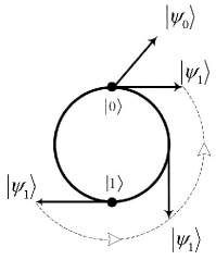
Figure 2: The graphical representation of the decomposition given by Eq.(54). After parallel transporting the vector $|\Psi_{1}\rangle$ from the south pole to the north pole, we can define an angle to quantify the difference between $|\Psi_{0}\rangle$ and $|\Psi_{1}\rangle$. This angle could be used to quantify the entanglement of the state $|\Psi\rangle$.

The condition (56) leads to the same conditions as given in Eq.(26). A natural definition of the entanglement is then given by

$$E=A\sum_{b,c,b^{\prime}c^{\prime}}\biggl{[}|t_{0bc}t_{1b^{\prime}c^{\prime}}-t_{0b^{\prime}c^{\prime}}t_{1bc}|^{2}+|t_{b0c}t_{b^{\prime}1c^{\prime}}-t_{b^{\prime}0c^{\prime}}t_{b1c}|^{2}+|t_{b0c}t_{b^{\prime}1c^{\prime}}-t_{b^{\prime}0c^{\prime}}t_{b1c}|^{2}\biggr{]}$$ (57)

where $A$ is a proper normalization factor and $t_{abc}\equiv\langle abc|\Psi\rangle$. The generalization of this definition is straightforward. This definition is exactly the same as the one discussed by Meyer et al.Meyer2002 .

IV.3.4 Quantifying Entanglement

Based on our discussion above, we are now in position to propose a quantity that quantifies the degree of entanglement of a 3-qubit state. As our discussion so far suggests, we need to probe for the entanglement of 3-qubits in a 1-qubit $\otimes$ 2-qubit state. (Subsequently, we can particularize to the fiber of the third hopf map and classify the degree of entanglement of the 2-qubit state.) We therefore partially trace two qubits to obtain the partially traced matrix $\rho_{1}$:

$$\rho_{1}=\frac{1}{2}\left(\begin{array}[]{cc}1+X_{9}&X_{1}-iX_{2}\\ X_{1}+iX_{2}&1-X_{9}\\ \end{array}\right)$$ (58)

Usually, for generic 3-qubit states, $\det\rho_{1}>0$. However, in the case of 2-qubit $\otimes$ 1qubit entanglement, the determinant of the matrix vanishes, and therefore $X_{3}=X_{4}=X_{5}=X_{6}=X_{7}=X_{8}=0$. It seems obvious then that we could use the quantity

$$E=X_{3}^{2}+X_{4}^{2}+X_{5}^{2}+X_{6}^{2}+X_{7}^{2}+X_{8}^{2}=1-X_{1}^{2}-X_{2}^{2}-X_{9}^{2}$$ (59)

to quantify entanglement. Small values of $E$ means high degree of separability of 1-qubit and 2-qubit Hilbert spaces in the 3-qubit state and viceversa. Notice that this quantity $E$ only measures the entanglement between the first qubit and the $2$-qubit system of second and third qubit. Similarly, we can construct the second or third qubit into base space to get two different constructions of the Hopf fibration. A more reasonable definition of the measurement of the entanglement will be the average of the quantity given in Eq.(59) over all possible constructions.

Let us now test these assumptions on two well known states, GHZ and W states of the 3-qubit problem. The generalized GHZ states read:

$$|GHZ\rangle|_{generalized}=\alpha_{0}|000\rangle+\gamma_{1}|111\rangle\;\;\;\Longrightarrow\;\;\;\begin{array}[]{c}X_{5}=2Re\gamma_{1}Im\alpha_{0}+2Im\gamma_{1}Re\alpha_{0}\\ X_{6}=2Re\gamma_{1}Re\alpha_{0}-2Im\gamma_{1}Im\alpha_{0}\\ X_{9}=|\alpha_{0}|^{2}-|\gamma_{1}|^{2}\\ \end{array}$$ (60)

the other $X$’s being zero, and with a degree of entanglement $E=1-|\alpha_{0}|^{2}+|\gamma_{1}|^{2}$. For the pure GHZ state $\alpha=\gamma_{1}=1/\sqrt{2}$ and therefore $E=1$, meaning that the GHZ state is a maximally entangled state of the 3 qubit system, consistent with well-known result.

The generalized W state reads:

$$|W\rangle_{generalized}=\delta_{0}|100\rangle+\beta_{0}|010\rangle+\alpha_{1}|001\rangle\;\;\;\Longrightarrow\;\;\;\begin{array}[]{c}X_{3}=2Re\alpha_{1}Re\delta_{0}-2Im\alpha_{1}Im\delta_{0}\\ X_{4}=2Im\alpha_{1}Re\delta_{0}+2Re\alpha_{1}Im\delta_{0}\\ X_{5}=2Re\beta_{0}Re\delta_{0}-2Im\beta_{0}Im\delta_{0}\\ X_{8}=2Im\beta_{0}Re\delta_{0}+2Re\beta_{0}Im\delta_{0}\\ X_{9}=|\alpha_{1}|^{2}+|\beta_{0}|^{2}-|\delta_{0}|^{2}\\ \end{array}$$ (61)

For the W state, $X_{3}=X_{5}=2X_{9}=\frac{2}{3}$ and the degree of entanglement is $E=X_{3}^{2}+X_{5}^{2}=8/9$, consistent with the literatureMeyer2002 .

IV.3.5 Conjecture

A natural question is whether this construction is generalizable to systems with more than 3 qubits. One can imagine expanding the same formalism by always adding another square root of unity and forming the next algebra. Although this is possible via the Cayley-Dickenson formalism (see Appendix), the algebras formed in this way are not alternative, and cannot be written as fibrations of spheres over sphere base spaces. The Hopf construction stops at octonions. However, the subsequent algebras, although not division, are nicely normed, which means that they have an inverse. So in principle the type of map that we give in this paper is possible. However, the map would fail in the following sense: it would be possible to map non-zero points into zeros in the base space, fact which is not possible in the maps using division algebra numbers. This is just a restatement of the fact that further algebras would have zero divisors.

However, the Cayley-Dickson construction, as well as the fact that the number of dimensions of the algebras created by this construction is identical to the number of dimensions of the qubit spaces, hint at some deeper connection between the Cayley construction and qubit states. Interestingly, this construction might be very related to the hyperdeterminant construction of Miyake and Wadatimiyake2003 . Out definition of the entanglement $E$ in Eq.(57) is very similar to the hyperderterminant construction. It would be interesting to investigate this correspondence for higher qubit states. The non-existence of Hopf maps for higher than 3 qubits seems to tell us that the 1-qubit, 2-qubit, and 3-qubit states are, in some sense, more special than higher qubit states. However, the richness of information that we are able to procure with the identification presented in this paper and in the paper by Mosseri and Dandoloff seems to make further investigation in this field worthy.

V Conclusions

In this paper we analyze the 3-qubit state. We give a full description of the 3-qubit Hilbert space by relating it to the third and last Hopf fibration. We prove that this fibration is entanglement sensitive, that is, it can detect whether the 3-qubit state is separable or entangled. Moreover, we show that one can define a quantity to describe the entanglement of the 3-qubit state and the possibility of it being separable as a 1-qubit$\otimes$ 2-qubit state. Our results, cumulated to the results of Mosseri, show that non-trivial fibrations are a very useful tool in describing many-qubit states and their entanglement.

VI Acknowledgements

This paper was the result of a suggestion by S.C. Zhang, for which we are deeply grateful. We also acknowledge private communications with Remy Mosseri, for which we are deeply grateful. The authors would like to thank G. Chapline, C.H.Chern, T. Cuk, J. Franklin, R.B. Laughlin, D. Santiago, T.-C. Wei, C.J. Wu, J. T. Yard and G. Zeltzer for valuable discussions. This work is supported by the NSF under grant numbers DMR-9814289 and 2FEV602, and the US Department of Energy, Office of Basic Energy Sciences under contract DE-AC03-76SF00515. The authors also acknowledge support from the Stanford Graduate Fellowship Program.

Appendix A Octonions and the last Division Algebra

An extensive review of octonions and division algebras is provided by Baezbaez . Real and Complex numbers are used by physicists daily. Although real numbers are in a sense ‘nicer’ than complex numbers because the conjugate of a real number is itself, complex numbers bring about new and powerful properties and structure. However, they are only the first two kind of numbers in a set of four possible structures. In a far-reaching and very deep argument, it has been proved that there are only four division algebras, in other words, there are only 4 vector spaces $A$ equipped with a bilinear map $m:\;A\times A\rightarrow A$ called multiplication, and with a non-zero element called unit such that $m(1,a)=m(a,1)=a$ (these properties form an algebra) and given $a,b\in A$ with $ab=0$ then either $a=0$ or $b=0$ (no zero divisors - property defining the division algebra). The real and the complexes ($\mathbb{R},\;\mathbb{C}$) form the first two division algebras. The third and fourth division algebra are the quaternions and the octonions ($\mathbb{Q},\;\mathbb{O}$). The Cayley-Dickson constructions provides a construction of the elements in $\mathbb{R},\;\mathbb{C},\;\mathbb{Q},\;\mathbb{O}$ which makes apparent the fact that each one fits nicely in the next. The complex numbers can be considered as a pair of real numbers $(a,b)$; then addition can be performed component-wise whereas the multiplication rule is:

$$(a,b)(c,d)=(ac-db,ad+cb)=ac-db+(ad+cb)i.$$ (62)

We can define the quaternions in a similar way: a quaternion is a pair of complex numbers $(a,b)$, with the complex conjugation and the multiplication laws being:

$$(a,b)^{\star}=(a^{\star},-b),\;\;\;\;\;(a,b)(c,d)=(ac-d^{\star}b,bc^{\star}+da)=ac-d^{\star}b+(bc^{\star}+da)i_{2}.$$ (63)

The quaternions are non-commutative and upon expansion, can be written as $q=Rea+i_{1}Ima+i_{2}Reb+i_{3}Imb$, $i_{1}^{2}=i_{2}^{2}=i_{3}^{2}=i_{1}i_{2}i_{3}=-1$. We can go one step further and build an octonion from a pair of quaternions $(q_{1},q_{2})$, with the multiplication and conjugation laws the same as before. The octonions are non-associative, as well as non-commutative. They are the biggest division algebra. If one continues the Cayley-Dickson construction further, by taking a pair of octonions, one discovers that the division property is lost, that is, the new numbers have zero divisors. The division algebras, including the non-associative octonions have the essential property that they are alternative, in other words:

$$\forall\;\;a,b\in\mathbb{R},\mathbb{C},\mathbb{Q},\mathbb{O}\;\;\Longrightarrow\;\;(aa)b=(aab),\;\;(ab)a=a(ba),\;\;(ba)a=b(aa).$$ (64)

Octonions can be presented in the double quaternion format but also, equivalently, in expanded format with $i_{1},i_{2},i_{3},i_{4},i_{6},i_{7}$ as imaginary units (square roots of $-1$):

$$o=x_{0}+\sum_{\alpha}x_{m}i_{m},\;\;\;\;x_{0,...,7}\in\mathbb{R},\;\;\;\;\;i_{1}^{2}=...=i_{7}^{2}=-1,$$ (65)

which can also be described in terms of quaternions and complex numbers as $o=\{(x_{0}+x_{1}i_{1})+(x_{2}+x_{3}i_{1})i_{2}\}+\{(x_{4}+x_{7}i_{1})+(x_{6}-x_{5}i_{1})i_{2}\}i_{4}$. The multiplication table can be given in terms of the cycles:

$$(123),\;\;(246),\;\;(435),\;\;(367),\;\;(651),\;\;(572),\;\;(714)$$ (66)

which read, for example $i_{7}i_{1}=i_{4}$, etc. The conjugate and inverse of an octonion $o$ is:

$$\bar{o}=x_{0}-\sum_{m}x_{m}i_{m},\;\;\;o^{-1}=\frac{\bar{o}}{|o|^{2}}.$$ (67)

Another way in which an octonion $o$ can be written is as a scalar $S(o)$ part and a vectorial $V(o)$ part:

$$S(o)=\frac{1}{2}(o+\bar{o})=x_{0},\;\;V(o)=\frac{1}{2}(o-\bar{o})=\sum_{m=1}^{7}V_{m}(o)i_{m}=\sum_{m=1}^{7}x_{i}i_{m}$$ (68)

An octonion $o$ can also be written in exponential form:

$$o=|o|\exp(\theta I),\;\;\theta=\arccos\left(\frac{S(o)}{|o|}\right),\;\;I=\frac{V(o)}{|V(o)|}$$ (69)

As presented in the body of the paper, the third hopf map is nicely presented in terms of octonions:

$$h_{1}:\begin{array}[]{ccc}\mathbb{O}\otimes\mathbb{O}&\longrightarrow&\mathbb{O}\cup\{\infty\}\approx S^{8}\\ (q_{1},q_{2})&\longrightarrow&h_{1}=o_{1}o_{2}^{-1}\\ \end{array},\;\;\;|o_{1}|^{2}+|o_{2}|^{2}=1$$ (70c)

$$h_{2}:\begin{array}[]{ccc}\mathbb{O}\cup\{\infty\}&\longrightarrow&S^{8}\\ h_{1}&\longrightarrow&X_{i,\;\;(i=1,...,9)}\\ \end{array},\;\;\;\;\sum_{i=1}^{9}X_{i}^{2}=1\;\;\;\;$$ (70f)

$$h_{2}\circ h_{1}(o_{1},o_{2})=X_{i}=\langle\sigma_{i}\rangle_{\Psi}=(o_{1}^{\star},o_{2}^{\star})\sigma_{i}\left(\begin{array}[]{c}o_{1}\\ o_{2}\\ \end{array}\right),$$ (70i)

where

$$\sigma_{1}=\left(\begin{array}[]{cc}0&1\\ 1&0\\ \end{array}\right),\sigma_{2,3,4,5,6,7,8}=\left(\begin{array}[]{cc}0&i_{1,2,3,4,5,6,7}\\ -i_{1,2,3,4,5,6,7}&0\\ \end{array}\right),\sigma_{9}=\left(\begin{array}[]{cc}1&0\\ 0&-1\\ \end{array}\right)$$ (77)

are a generalization of the Pauli matrices to Quternionic space. The form of the map is identical to the form of the map presented in Mosseri et alMosseri2001 . However, proving that $S^{7}$ is the fiber of this map turns out to be non-trivial, since as opposed to the quaternionic case of the second Hopf map, we lose the associativity property and therefore $(o_{1}o_{2})o_{3}\neq o_{1}(o_{2}o_{3})$ for $o_{1},o_{2},o_{3}\in\mathbb{O}$. However, after some explicit calculations one can find out that the essential property is that the algebra be alternative. Alternativity holding, one can prove the following: $o_{1}^{-1}(o_{1}o_{2})=(o_{1}^{-1}o_{1})o_{2}$ and therefore inverse map is:

$$h_{1}^{-1}(y)=\left(\begin{array}[]{c}\{(yd,d)\;|\;d\in\mathbb{O},\;\;|yd,d|=1\},\;\;x\neq\infty\\ \{(c,0)\;|\;c\in\mathbb{O},\;\;|c|=1,\;\;x=\infty\\ \end{array}\right)$$ (78)

References

- (1) Remy Mosseri and Rossen Dandoloff, J. Phys. A, 34 10243 (2001).
- (2) A. Einstein, B. Podolsky and N. Rosen, Phys. Rev. 47, 777 (1935).
- (3) C.H. Bennett, G. Brassard, C. Crepeau, R. Joza, A. Peres, and W.K. Wootters, Phys. Rev. Lett. 70, 1895 (1993).
- (4) C.H. Bennett and S. Wiesner, Phys. Rev. Lett. 69, 2881 (1992).
- (5) A.K. Ekert, Phys. Rev. Lett. 67, 661 (1991).
- (6) A.K. Ekert, J.G. Rarity, P.R. Tapster, and G.M. Palma, Phys. Rev. Lett. 69, 1293 (1992).
- (7) D. M. Greenberger, M. A. Horne and A. Zeilinger, in Bell’s Theorem, Quantum Theory and Conceptions of the Universe, edited by M. Kafatos (Kluwer Academic, Dordrecht, 1989), p.69.
- (8) S. Bose, V. Vedral, and P.L. Knight, Phys. Rev. A 57, 822 (1998).
- (9) M. Hillery, V. Buzek, and A. Berthiaume, Phys. Rev. A 59, 1829 (1999).
- (10) M. Kus and K. Zyczkowski, Phys. Rev. A, 59 032307 (1991).
- (11) H.A.Carteret and A. Sudbery, J. Phys. A, 33 4981 (2000).
- (12) C.H.Bennet, et al, Phys. Rev. A, 53, 2046 (1996); C.H.Bennet, et al, Phys. Rev. A, 54, 3824 (1996); V. Vedral et al, Phys. Rev. Lett., 78, 2275 (1997); V. Vedral et al, Phys. Rev. A, 56, 4452 (1997); V. Vedral et al, Phys. Rev. A, 57, 1619 (1998); M. Horodecki, et al, Phys. Rev. lett., 80, 5239 (1998); E.M.Rains, et al, Phys. Rev. A, 60, 179 (1999); S. Hill and W.K. Wootters, Phys. Rev. Lett., 78, 5022 (1997); W.K.Wootters, Phys. Rev. Lett., 80, 2245 (1998); A. F. Abouraddy, et al, Phys. Rev. A, 64 050101 (2001).
- (13) M. Lewenstein, et al, J. Mod. Opt., 47 2481 (2001).
- (14) M. Horodecki, et al, e-print quant-ph/0006071.
- (15) D. A. Meyer and Nolan R. Wallach, J. Math Phys., 43 4273 (2002).
- (16) J. C. Baez, Bull. Amer. Math. Soc. 39 145 (2002).
- (17) A. Miyake, Phys. Rev. A 67, 012108 (2003). A.Miyake and M. Wadati, quant-ph/0212146.