Concepts and methods in the theory of open quantum systems

Abstract

The central physical concepts and mathematical techniques used in the theory of open quantum systems are reviewed. Particular emphasis is laid on the interrelations of apparently different approaches. Starting from the appropriate characterization of the quantum statistical ensembles naturally arising in the description of open quantum systems, the corresponding dynamical evolution equations are derived for the Markovian as well as for the non-Markovian case.

1 Introduction

Perfect isolation of quantum systems is not possible since any realistic system is influenced by the coupling to an environment, which typically has a large number of degrees of freedom. A prototypical physical system illustrating this situation is given by an atom interacting with the surrounding radiation field Cohen .

In general, a complete microscopic description of the degrees of freedom of the environment is too complicated. Hence, one has to look for more simple descriptions of the dynamics of the open system. In principle, one should investigate the unitary dynamics of the total system, i.e. system and environment, to obtain informations about the reduced system of interest by averaging the appropriate observables over the degrees of freedom of the environment. This is the main concern of the theory of open quantum systems TheWork .

Applications of the theory of open quantum systems are found in almost all areas of physics, ranging from quantum optics WallsMilburn to solid state physics Weiss , from chemical physics Pechukas to nanotechnology Kulik , from quantum information Nielsen to spintronics Loss . On a more fundamental level, the theory of open quantum systems is relevant for quantum measurement theory Braginsky and for decoherence and the emergence of classicality Giulini .

Usually, the dynamics of an open quantum system is described in terms of the reduced density operator which is obtained from the density operator of the total system by tracing over the variables of the environment. In order to eliminate the degrees of freedom of the environment various approximations are needed which lead to a closed equation of motion for the density matrix of the open system. The most famous one being the Markov approximation which eventually leads to a so-called quantum master equation which, in turn, generates a quantum dynamical semi-group in the space of reduced density matrices Alicki . Prominent representants of such equations are the quantum optical master equation, and, derived under slightly different assumptions, the quantum Brownian motion master equation, with applications in condensed matter physics.

For stronger couplings between the system and the environment the finite relaxation time of the environment may significantly influence the dynamics of the open system, making necessary a non-Markovian treatment of the reduced system dynamics. Typical examples of such a behaviour arise in condensed matter physics at low temperatures Weiss . There are several strategies to go beyond a Markovian description of open quantum systems. Prominent approaches are provided by the influence functional technique Weiss , the cumulant expansion Royer1 ; Royer2 ; VanKampen and projection operator techniques Nakajima ; Zwanzig ; Chaturvedi .

During the past decade another approach to the description of open quantum systems has emerged, essentially motivated by the experimental evidence for quantum jumps in simple three-level ions Cook and similarly in the photon excitation number of a single mode of a high-Q cavity Walther . The common feature of these experiments is that they can be described within the theory of continuous measurements Braginsky . Under the condition that the information extracted from the system by the environment is recoverable, alternative measurement schemes give rise to different stochastic processes for the wave function of the open system Carmichael . For example, the direct photon counting of the light emitted by an excited atom gives rise to a piecewise deterministic process for the wave function of the atom. On this selective level of description of open quantum systems the typical stochastic processes arising are Markovian. The relation between the selective wave function approach and the non-selective density matrix approach is simply stated TheWork : The covariance of the stochastic wave function is the density matrix of the reduced system.

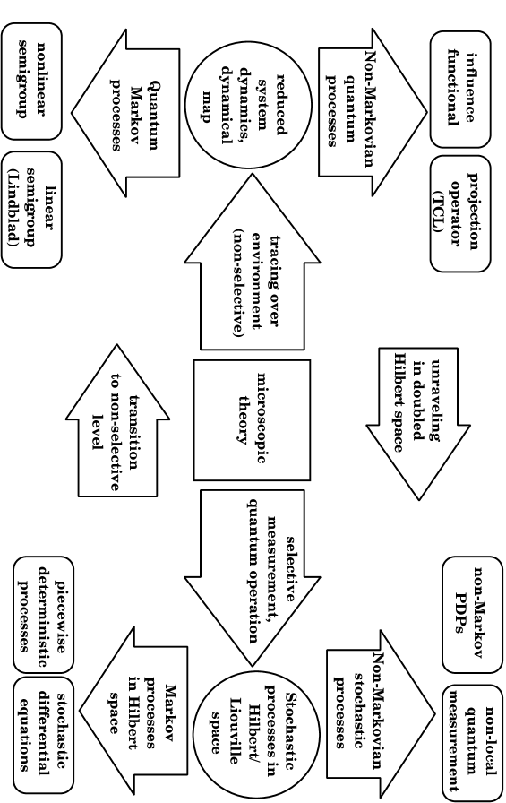
Figure 1: Basic concepts and methods used in the theory of open quantum systems.

The aim of the paper is to guide the reader in a systematic way through the different levels of description available for the investigation of the dynamics of open quantum systems: Density matrix and wave function approaches, selective and non-selective measurements, Markovian and non-Markovian approximations, quantum optical and quantum Brownian motion master equations, linear and non-linear semigroups, piecewise deterministic and diffusive processes for the wave function. Particular emphasis will be laid on establishing relationships between apparently different approaches. For this reason the paper concentrates on the explanation of the flow diagram Fig. 1 which summarizes in a schematic and simplified way the main aspects of the theory of open quantum systems. The structure of the paper reflects the main paths through the flow diagram Fig. 1. In Sec. 2 we discuss the centre of the figure, i.e. the microscopic description of the dynamics of open systems. In Sec. 3 we proceed anti-clockwise from the centre of the figure to the left, and show how dynamical maps and quantum Markov processes arise. In Sec. 4 we take the opposite path (clockwise from the centre to the right) and discuss quantum operations, continuous measurements and stochastic processes in Hilbert space. Finally, in Sec. 5 we describe the upper part of the flow diagram, i.e. the non-Markovian theory, proceeding clockwise from the centre to the left through the upper half of the figure.

2 Dynamics of open systems: Microscopic theory

In general terms, an open quantum system is a quantum mechanical system $S$ with Hilbert space ${\cal{H}}_{S}$ which is coupled to another quantum system $B$, the environment, with Hilbert space ${\cal{H}}_{B}$. Thus, $S$ is a subsystem of the total system $S+B$ living in the tensor product space ${\cal{H}}_{S}\otimes{\cal{H}}_{B}$. Sometimes, the surroundings $B$ of the open system are termed reservoir to denote an environment with an infinite number of degrees of freedom. If the reservoir is in thermal equilibrium one speaks of a heat bath.

Let us denote by $H_{S}$ the Hamiltonian of the open system, by $H_{B}$ the free Hamiltonian of the environment, and by $H_{I}$ the Hamiltonian describing the interaction between the system and the environment. The Hamiltonian of the total system can then be written as

$$H=H_{S}\otimes I_{B}+I_{S}\otimes H_{B}+\alpha H_{I},$$ (1)

where $I_{S}$ and $I_{B}$ denote the identities in the Hilbert spaces of the system and of the environment, respectively, and $\alpha$ is a coupling constant. The dynamics of the coupled system $S+B$ is thus assumed to be Hamiltonian.

An open system $S$ is singled out by the fact that all observables $A$ of interest refer to this system. Such observables are of the form $A\otimes I_{B}$, where $A$ acts in the Hilbert space of the open system. If the state of the total system $S+B$ is described by some density matrix $\rho$, then the expectation value of the observable $A$ is determined by

$$\langle A\rangle=\mathrm{tr}_{S}\{A\rho_{S}\},$$ (2)

where

$$\rho_{S}=\mathrm{tr}_{B}\rho$$ (3)

is the reduced density matrix. In the above equations $\mathrm{tr}_{S}$ and $\mathrm{tr}_{B}$ denote, respectively, the partial traces over the degrees of freedom of the open system $S$ and of the environment $B$. The reduced density matrix is of central interest for the theory of open quantum systems. As we mentioned, the total density matrix evolves unitarily and, hence, the time-development of the reduced density matrix may be represented in the form

$$\rho_{S}(t)=\mathrm{tr}_{B}\left\{U(t,0)\rho(0)U^{\dagger}(t,0)\right\},$$ (4)

where the initial state of the total system at time $t=0$ is given by $\rho(0)$ and $U(t,0)$ is the time-evolution operator of the total system over the time interval from $t=0$ to $t>0$. The corresponding differential form of the evolution is obtained from a partial trace over the environment of the von Neumann equation,

$$\frac{d}{dt}\rho_{S}(t)=-i\mathrm{tr}_{B}[H(t),\rho(t)].$$ (5)

In the following we will survey the most important approaches and approximations to the above exact equation of motion. To this end we will first describe the paths starting from the centre of the flow diagram Fig. 1 to the left and to the right through the lower part of the figure.

3 Dynamical maps and quantum Markov processes

Figure 2: Schematic overview of the cases in which a Markovian quantum master equation can be derived from an underlying microscopic theory.

Given that the initial state is of the form $\rho(0)=\rho_{S}(0)\otimes\rho_{B}$, the dynamics expressed through Eq. (4) can be viewed as a map of the state space of the reduced system which maps the initial state $\rho_{S}(0)$ to the state $\rho_{S}(t)$ at time $t\geq 0$,

$$\rho_{S}(0)\mapsto\rho_{S}(t)=V(t)\rho_{S}(0).$$ (6)

For a fixed $t$ this map is known as dynamical map. Considered as a function of time $t$ it provides a one-parameter family $\{V(t)|t\geq 0\}$ of dynamical maps. If the characteristic time scale over which the reservoir correlation functions decay are much smaller than the characteristic time scale of the system’s relaxation, it is justified to neglect memory effects in the reduced system dynamics and one expects a Markovian type behaviour, which may be formalized by the semi-group property

$$V(t_{1})V(t_{2})=V(t_{1}+t_{2}),\quad t_{1},t_{2}\geq 0.$$ (7)

The one-parameter family of dynamical maps then becomes a quantum dynamical semi-group. Introducing the corresponding generator $\mathcal{L}$ one immediately obtains an equation of motion for the reduced density matrix of the open system of the form

$$\frac{d}{dt}\rho_{S}(t)=\mathcal{L}\rho_{S}(t).$$ (8)

Such an equation is called a Markovian quantum master equation. The most general form of the generator $\mathcal{L}$ is provided by a theorem due to Gorini, Kossakowski and Sudarshan Gorini and by a theorem of Lindblad Lindblad according to which

$$\mathcal{L}\rho_{S}=-i[H,\rho_{S}]+\sum_{i}\gamma_{i}\left(A_{i}\rho_{S}A^{\dagger}_{i}-\frac{1}{2}A^{\dagger}_{i}A_{i}\rho_{S}-\frac{1}{2}\rho_{S}A^{\dagger}_{i}A_{i}\right).$$ (9)

Here, $H$ is the generator of the coherent part of the evolution (which need not be identical to the free Hamiltonian of the system) and the $A_{i}$ are system operators with corresponding relaxation times $\gamma_{i}$. Eq. (8) with this form of the generator is often referred to as Lindblad equation. In a number of physical situations a quantum master equation whose generator is exactly of the Lindblad form can be derived from the underlying microscopic theory under certain approximations. The most important cases are the weak-coupling limit, the singular coupling limit and the low density limit (see Fig. 2).

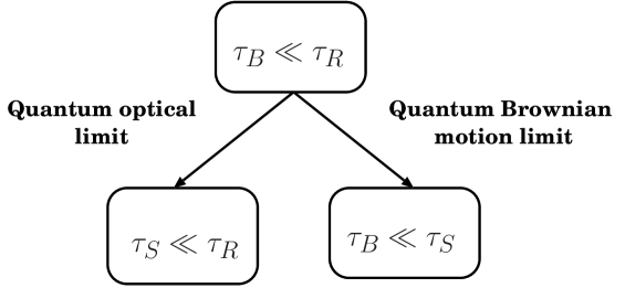
Figure 3: A comparison of the typical time scales arising in the microscopic derivations of the quantum optical and the quantum Brownian motion limit of the quantum master equation. $\tau_{B}$ denotes the correlation time of the environment, $\tau_{R}$ the relaxation time of the open system, and $\tau_{S}$ the time scale of its systematic evolution.

A widely used Markovian quantum master equation that can be derived from a microscopic Hamiltonian for the total system in the weak-coupling limit is the quantum optical master equation WallsMilburn . The central assumption underlying the weak-coupling approximation is that the times scales of the system’s relaxation $\tau_{R}$ and of the correlation time of the environment $\tau_{B}$ are clearly separated, i.e. $\tau_{B}\ll\tau_{R}$. One further essential approximation entering the derivation of the quantum optical master equation is the so-called rotating wave approximation. The physical condition behind this approximation is the following one: The time scale $\tau_{S}$ of the systematic evolution of the reduced system is small compared to its relaxation time $\tau_{R}$, i.e. $\tau_{S}\ll\tau_{R}$. Unfortunately, this condition is violated in many physical applications involving stronger couplings and low temperatures. It occurs that the systematic dynamics of the reduced system may even by slow compared to the correlation time of the environment, that is $\tau_{B}\ll\tau_{S}$. Such cases lead to the so-called quantum Brownian motion master equation Gardiner (see Fig. 3).

In the treatment of open many-body systems one also encounters non-linear quantum master equations for the reduced one-particle density matrix AlickiMesser . In many cases the corresponding generator takes on the structure of a Lindblad generator whose coefficients depend parametrically on the density matrix. This means that the generator $\mathcal{L}=\mathcal{L}[\rho_{S}]$ provides a super-operator which represents a function of $\rho_{S}$ and which is of Lindblad form for each fixed argument. This immediately leads to a master equation of the general form

$$\frac{d}{dt}\rho_{S}(t)=\mathcal{L}[\rho_{S}(t)]\rho_{S}(t).$$ (10)

Some prominent examples of non-linear quantum master equations are shown in Fig. 4. At this point we arrived at the lower left corner of Fig. 1. Now we go back to the centre of the figure and will explain why it might be necessary to follow the clockwise path from the centre to the right.

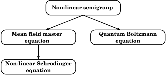
Figure 4: Schematic overview of typical non-linear semi-groups. A typical example for a mean-field equation are the laser equations and an example for the application of the non-linear Schrödinger equation is super-radiance.

4 Quantum operations, continuous measurements and stochastic processes in Hilbert space

In order to extract information from a quantum system a measurement must be carried out. Let us consider the situation that an open system is measured through an indirect measurement on its environment. Thus, the open system is the quantum object to be measured, while the environment plays the role of the quantum probe. The latter is measured by means of a classical apparatus, once correlations between object and probe system are created as a result of their interaction.

Let us assume that the interaction between the open system and the environment begins at time $t=0$. At this time the state of the system is characterized by the density matrix $\rho_{S}$ and the state of the environment, the quantum probe, is given by

$$\rho_{B}=\sum_{k}p_{k}|\phi_{k}\rangle\langle\phi_{k}|.$$ (11)

The initial density matrix of the total system is thus $\rho(0)=\rho_{S}\otimes\rho_{B}$. At time $\tau$ a classical measurement apparatus measures the bath observable

$$R=\sum_{m}r_{m}|\varphi_{m}\rangle\langle\varphi_{m}|,$$ (12)

the spectrum of which is assumed to be discrete and non-degenerate, for simplicity. The application of the von Neumann-Lüders projection postulate to the classical measuring device shows that the reduced system’s state after the measurement is given by

$$\rho^{\prime}_{m}=P(m)^{-1}\Phi_{m}(\rho_{S}),$$ (13)

where

$$\Phi_{m}(\rho_{S})=\sum_{k}\Omega_{mk}\rho_{S}\Omega^{\dagger}_{mk},$$ (14)

with

$$\Omega_{mk}=\sqrt{p_{k}}\langle\varphi_{m}|U|\phi_{k}\rangle,$$ (15)

and

$$P(m)=\mathrm{tr}_{S}\{\Phi_{m}(\rho_{S})\}.$$ (16)

In these formulae $U$ is the time-development operator of the total system describing the coupled evolution of quantum system and quantum probe. The probability that the measurement outcome is $r_{m}$ is given by $P(m)$. Under the condition that the outcome is $r_{m}$, the corresponding transformation of the reduced system’s density matrix from the initial state $\rho_{S}$ to the new state $\rho^{\prime}_{m}$ is provided by the map $\Phi_{m}(\rho_{S})$ which is known as a quantum operation. Like the dynamical map (6) it represents a convex-linear and completely positive map. The representation (14) in terms of the operators $\Omega_{mk}$ takes on the general form required by the representation theorem of quantum operations Krauss .

When writing Eq. (13) it is assumed that the measurement is a selective one, i.e. that after the measurement the information on the measurement outcomes is retained. Therefore, the original ensemble described by $\rho_{S}$ is split into a number of sub-ensembles described by the various $\rho^{\prime}_{m}$, each sub-ensemble being conditioned on a specific outcome $r_{m}$. By contrast, in the case of a non-selective measurement the final state of the system after the measurement is given by

$$\rho^{\prime}=\sum_{m}P(m)\rho^{\prime}_{m}=\sum_{m}\Phi_{m}(\rho_{S}),$$ (17)

which describes the ensemble obtained after re-mixing the sub-ensembles after the measurement. Thus, the first important step in the description of an open quantum system is to make clarity about the type of measurement which is performed in order to obtain information about the system. In other words, we have to know whether the (indirect) measurement is selective or not. The microscopic theory of the total (closed) system has to be supplemented with this information as is indicated in Fig. 1. This important distinction has fundamental consequences on the choice of the formalism required to describe the open system. In fact, selective and non-selective measurements require different characterizations of the quantum statistical properties of the open system.

Let us now follow another important path through the flow diagram. Again we start at the centre of Fig. 1 and proceed clockwise to the right into the lower part of the diagram. The decisive aspect of this path is the indirect selective measurement of the open quantum system, which requires a particular characterization of the quantum statistical ensembles.

A quantum statistical ensemble characterized in terms of a density matrix $\rho$ describes a disordered set of a large number of individual quantum systems, where each system has been prepared in one of a certain set of states $\psi_{\alpha}$. The preparation measurements could have been carried out, for example, through the measurements of complete sets of commuting observables. The various $\psi_{\alpha}$, however, need not be orthogonal. A mixture of these states with respective weights $w_{\alpha}$ gives rise to an ensemble $\mathcal{E}_{\rho}$ which is described by the density matrix

$$\rho=\sum_{\alpha}w_{\alpha}|\psi_{\alpha}\rangle\langle\psi_{\alpha}|.$$ (18)

A different kind of ensembles which is appropriate for the description of selective measurements and which will be denoted by ${\mathcal{E}}_{P}$ is obtained as follows. Consider a collection of pure quantum statistical ensembles ${\mathcal{E}}_{\alpha}$ describable by corresponding states $\psi_{\alpha}$. We want to keep, as required for a selective measurement, the information that a particular quantum system belongs to a particular ensemble ${\mathcal{E}}_{\alpha}$. For this purpose we take $N_{\alpha}$ identically prepared copies ${\mathcal{E}}^{(1)}_{\alpha},{\mathcal{E}}^{(2)}_{\alpha},\ldots,{\mathcal{E}}^{(N_{\alpha})}_{\alpha}$ of ${\mathcal{E}}_{\alpha}$ for each ${\alpha}$. The new ensemble ${\mathcal{E}}_{P}$ is then the collection of these ensembles, that is an ensemble of ensembles:

$${\mathcal{E}}_{P}=\left\{{\mathcal{E}}^{(1)}_{1},\ldots,{\mathcal{E}}^{(N_{1})}_{1},{\mathcal{E}}^{(1)}_{2},\ldots,{\mathcal{E}}^{(N_{2})}_{2},\ldots,{\mathcal{E}}^{(1)}_{\alpha},\ldots,{\mathcal{E}}^{(N_{\alpha})}_{\alpha},\ldots\right\}.$$ (19)

The numbers $N_{\alpha}$ are chosen such that $w_{\alpha}=N_{\alpha}/N$, where $N=\sum_{\alpha}N_{\alpha}$, which implies that ${\mathcal{E}}_{\alpha}$ appears with the statistical weight $w_{\alpha}$ in the set (19). The decisive distinction of an ${\mathcal{E}}_{P}$-ensemble to an $\mathcal{E}_{\rho}$-ensemble is that ${\mathcal{E}}_{P}$ represents a set whose elements are again sets, namely the ensembles ${\mathcal{E}}^{(i)}_{\alpha}$. A schematic picture of an ensemble of type $\mathcal{E}_{P}$ is given in Fig. 5.

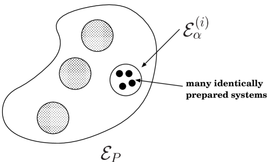
Figure 5: Schematic representation of an ensemble of type $\mathcal{E}_{P}$.

Since the various ${\mathcal{E}}_{\alpha}$ making up ${\mathcal{E}}_{P}$ are represented by their corresponding state vector $\psi_{\alpha}$, an ensemble of the type ${\mathcal{E}}_{P}$ gives rise to a probability distribution $P=P[\psi]$ on Hilbert space ${\mathcal{H}}_{S}$. Consequently, the state vector becomes a random vector in Hilbert space (see TheWork and references therein). More precisely speaking, the functional $P[\psi]$ represents a probability distribution on projective Hilbert space, that is on the space of rays in ${\mathcal{H}}_{S}$. Regarded as a density functional on $\mathcal{H}_{S}$, the distribution $P[\psi]$ is therefore subjected to the normalization condition

$$\int D\psi D\psi^{\ast}P[\psi]=1,$$ (20)

with an appropriate volume element $D\psi D\psi^{\ast}$ in Hilbert space, it vanishes outside the unit sphere $||\psi||=1$ in Hilbert space, and it is invariant under changes of the phase of the state vector, that is $P[\exp(i\chi)\psi]=P[\psi]$. The density matrix $\rho$ characterizing the corresponding ensemble $\mathcal{E}_{\rho}$ now appears as the covariance matrix of the random state vector $\psi$ which is defined as the expectation value E of the quantity $|\psi\rangle\langle\psi|$. In terms of the probability density functional $P[\psi]$ we have

$$\rho={\rm{E}}\left[|\psi\rangle\langle\psi|\right]\equiv\int D\psi D\psi^{\ast}P[\psi]|\psi\rangle\langle\psi|.$$ (21)

This relation clearly reveals that the statistics of an ensemble $\mathcal{E}_{\rho}$ is completely determined by the probability density $P[\psi]$, while the converse is obviously not true.

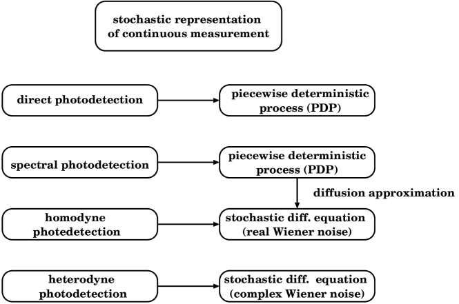
Figure 6: Different continuous measurement schemes give rise to different Markovian stochastic processes for the wave function of the reduced system. The stochastic Schrödinger equations are obtained as diffusion limits of appropriate piecewise deterministic processes.

The formalism of probability densities on Hilbert space now allows the description of the dynamics of an open system which is continuously monitored through its environment (see the lower part of the flow diagram shown in Fig. 1). The probability density then becomes a time-dependent functional $P=P[\psi,t]$ and the reduced system’s state vector provides a stochastic process $\psi(t)$ in Hilbert space. Physically, $\psi(t)$ represents the state of the reduced system which is conditioned on a specific readout of the measurement carried out on the environment. Consequently, the stochastic evolution depends on the measurement scheme used to monitor the environment. As an example we write a stochastic differential equation corresponding to the Lindblad equation (8) with generator (9):

$$d\psi(t)=-iG(\psi(t))dt+\sum_{i}\left(\frac{A_{i}\psi(t)}{||A_{i}\psi(t)||}-\psi(t)\right)dN_{i}(t).$$ (22)

A stochastic differential equation of this form is known as a piecewise deterministic process. The first term on the right-hand side describes the deterministic evolution periods given by the non-linear Schrödinger equation

$$\frac{d}{dt}\psi=-iG(\psi)\equiv H\psi-\frac{i}{2}\sum_{i}\gamma_{i}\left(A_{i}^{\dagger}A_{i}-||A_{i}\psi||^{2}\right)\psi.$$ (23)

The deterministic pieces of the motion are interrupted by instantaneous changes of the state vector according to $\psi\longrightarrow A_{i}\psi/||A_{i}\psi||$. These so-called quantum jumps are described by the second term on the right-hand side of Eq (22) which involves the random numbers $dN_{i}(t)$. These numbers take on the values $0$ or $1$ and represent independent Poisson increments with the expectation values

$${\rm{E}}\left[dN_{i}(t)\right]=\gamma_{i}||A_{i}\psi(t)||^{2}dt.$$ (24)

A stochastic evolution equation of this form is obtained, for example, if the reduced system represents an excited atom, the environment is an electromagnetic field vacuum and the system’s state is monitored through the direct observation of the emitted quanta.

Depending on the measurement scheme, it may be appropriate to perform a diffusion approximation of the above piecewise deterministic process. This leads to a diffusion process for the wave function of the reduced system involving real or complex Wiener noise. An overview of the Markov processes for the wave function of the open system related to a certain continuous measurement scheme is given in Fig. 6.

5 Non-Markovian processes

Let us now turn our attention to the description of the non-Markovian dynamics of an open quantum system. We proceed counter clockwise as indicated in the upper half of the flow diagram shown in Fig. 1. Again, the starting point is provided by an underlying microscopic theory for the total system. Unlike in the Markovian case, the first step consists in deriving an exact equation of motion for the reduced density matrix of the open system through an elimination of the dynamical variables of the environment. Of course, a closed analytical expression for the reduced density matrix can be obtained only for a few analytically solvable models, such as for the damped harmonic oscillator and for free Brownian motion FeynmanVernon ; CALDEIRA ; GRABERT . In many interesting cases, however, exact representations for the reduced density matrix serve as starting points of a perturbation expansion in the system-environment coupling and of the development of numerical integration schemes.

As indicated in Fig. 1 and in more detail in Fig. 7 there are several possibilities to carry out this program. Probably the most prominent one is to use the Nakajima-Zwanzig projection operator technique Nakajima ; Zwanzig . In this approach one derives a formally exact equation for the reduced density matrix of the open system in the form of an integro-differential equation involving a certain memory kernel. The practical disadvantage of this approach is that the perturbation expansion of the memory kernel does not simplify the convolution structure of the equations whose numerical solution could be quite involved (see also Royer2 ).

As far as a numerical and/or perturbation approach is concerned a more appropriate strategy is to derive a time-local master equation for the open system’s density matrix $\rho_{S}(t)$ which takes the form

$$\frac{d}{dt}\rho_{S}(t)={\mathcal{K}}(t)\rho_{S}(t).$$ (25)

${\mathcal{K}}(t)$ is a time-dependent generator, a super-operator in the reduced system’s Hilbert space ${\mathcal{H}}_{S}$. Employing the time-convolutionless (TCL) projection operator technique Shibata1 ; Shibata2 one can show that a master equation of the form (25) indeed exists for small and intermediate couplings in the case of factorizing initial conditions. We remark that a similar method can also be used in the general case of a correlated initial state, in which case the time-local master equation contains an additional inhomogeneous term. It should be noted that Eq. (25) is local in time, i. e. that it does not involve an integration over the past history of the reduced system. Due to the explicit time-dependence of the TCL generator ${\mathcal{K}}(t)$, however, it does not lead to a quantum dynamical semigroup and, therefore, the generator need not be in Lindblad form.

Eq. (25) provides an appropriate starting point for a perturbation expansion with respect to some coupling parameter $\alpha$. To this end, one expands the time-local generator in powers of $\alpha$,

$${\mathcal{K}}(t)=\sum_{n=1}^{\infty}\alpha^{n}{\mathcal{K}}_{n}(t),$$ (26)

and solves the corresponding equation of motion which is obtained in the desired order in $\alpha$ either analytically or numerically. Such an expansion may be found in two different ways. One way is to start from the formal solution of the von Neumann equation of the total system and to use an expansion in terms of ordered cumulants Royer1 ; Royer2 ; VanKampen . Another way is to invoke the Feynman-Vernon influence functional representation of the reduced density matrix FeynmanVernon and to obtain an expansion of the generator directly in terms of the influence phase. Both strategies, where applicable, yield identical expansions of the TCL generator BMP_MQC2 . The different approaches to the description of the non-Markovian dynamics of an open system are summarized in Fig. 7.

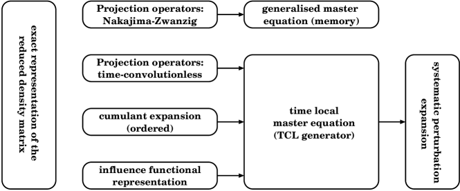
Figure 7: Schematic overview of the different approaches to the description of the non-Markovian dynamics of open quantum systems.

In general, one expects that a time-local master equation whose generator consists of only the first few terms of the expansion provides a good description of the reduced dynamics for weak and moderate couplings. However, it should be emphasized that an expansion of the form (26) need not exist for strong couplings. What happens in these cases is that the initial state $\rho_{S}(0)$ is not uniquely determined by the state $\rho_{S}(t)$ at time $t$. Specific examples of the application of this technique to physical models and of the breakdown of the TCL expansion in the strong coupling regime are discussed in TheWork .

Within any given order the time-local master equation for the reduced density matrix $\rho_{S}(t)$ which results from the above procedure takes the following form,

$$\frac{d}{dt}\rho_{S}(t)=A(t)\rho_{S}(t)+\rho_{S}(t)B^{\dagger}(t)+\sum_{i}C_{i}(t)\rho_{S}(t)D_{i}^{\dagger}(t),$$ (27)

with some time-dependent linear operators $A(t)$, $B(t)$, $C_{i}(t)$ and $D_{i}(t)$. This equation is linear in $\rho_{S}(t)$ and local in time, but it needs not be in Lindblad form. However, it is important to realize that a stochastic representation of the dynamics given by this equation is possible BKP99 ; TheWork .

The key point for a stochastic unraveling of the non-Markovian master equation (27) is the usage of a stochastic process in the doubled Hilbert space ${\mathcal{H}}_{S}\oplus{\mathcal{H}}_{S}$. This means that we represent the dynamics through a pair of stochastic wave functions

$$\theta(t)=\left(\begin{array}[]{c}\phi(t)\\ \psi(t)\end{array}\right),$$ (28)

such that $\theta(t)$ becomes a stochastic process in the doubled Hilbert space. An appropriate stochastic differential equation for a piecewise deterministic process in the doubled Hilbert space is the following,

$$d\theta(t)=-iG(\theta,t)dt+\sum_{i}\left(\frac{\|\theta(t)\|}{\left\|J_{i}(t)\theta(t)\right\|}J_{i}(t)\theta(t)-\theta(t)\right)dN_{i}(t).$$ (29)

The numbers $dN_{i}(t)=0,1$ are again independent Poisson increments with expectation values

$${\rm{E}}[dN_{i}(t)]=\frac{\left\|J_{i}(t)\theta(t)\right\|^{2}}{\|\theta(t)\|^{2}}dt,$$ (30)

and the non-linear operator $G(\theta,t)$ is defined as

$$G(\theta,t)=i\left(F(t)+\frac{1}{2}\sum_{i}\frac{\left\|J_{i}(t)\theta(t)\right\|^{2}}{\|\theta(t)\|^{2}}\right)\theta(t),$$ (31)

with time-dependent operators of block structure,

$$F(t)=\left(\begin{array}[]{cc}A(t)&0\\ 0&B(t)\end{array}\right),\quad J_{i}(t)=\left(\begin{array}[]{cc}C_{i}(t)&0\\ 0&D_{i}(t)\end{array}\right).$$ (32)

With the help of the calculus of piecewise stochastic processes TheWork it can now be demonstrated that the expectation value

$$\rho_{S}(t)={\rm{E}}\left[|\phi\rangle\langle\psi|\right]$$ (33)

satisfies the non-Markovian master equation (27). Thus, any time-local master equation allows a stochastic unraveling in the doubled Hilbert space. This fact makes it possible to use the apparatus of stochastic processes in the analysis of non-Markovian quantum processes and to design the corresponding stochastic simulation algorithms. It also enables us to close, finally, the flow diagram shown in Fig. 1 through the path following the upper half of the diagram.

References

- (1) C. Cohen-Tannoudj, J. Dupont-Roc, G. Grynberg, Atom-Photon Interactions (John Wiley, New York, 1998).
- (2) H. P. Breuer and F. Petruccione, The Theory of Open Quantum Systems (Oxford University Press, Oxford, 2002).
- (3) D. F. Walls and G. J. Milburn, Quantum Optics (Springer-Verlag, Berlin, 1994).
- (4) U. Weiss, Quantum Dissipative Systems, Volume 2 of Series in Modern Condensed Matter Physics (World Scientific, Singapore, 1999).
- (5) P. Pechukas and U. Weiss (guest editors), Quantum Dynamics of Open Systems, Chemical Physics, Special Issue, Vol. 268, Nos. 1-3 (2001).
- (6) I. O. Kulik and R. Ellialtioglu (Eds.), Quantum Mesoscopic Phenomena and Mesoscopic Devices in Microelectronics, NATO Series, Series C: Mathematical and Physical Sciences, Vol. 559 (Kluwer Academic Publishers, Dordrecht, 2000).
- (7) M. A. Nielsen and I. L. Chuang, Quantum Computation and Quantum Information (Cambridge University Press, Cambridge, 1997).
- (8) D.D. Awschalom, D. Loss, and N. Samarth (eds.), Semiconductor Spintronics and Quantum Computation, Series on Nanoscience and Technology, (Springer-Verlag, Berlin, 2002).
- (9) V. B. Braginsky and F. Ya. Khalili, Quantum Measurement (Cambridge University Press, Cambridge, 1992).
- (10) D. Giulini, E. Joos, C. Kiefer, J. Kupsch, I.-O.Stamatescu, H. D. Zeh, Decoherence and the Appearance of a Classical World in Quantum Theory (Springer-Verlag, Berlin, 1996).
- (11) R. Alicki and M. Fannes, Quantum Dynamical Systems (Oxford University Press, Oxford, 2001).
- (12) A. Royer, Phys. Rev. A, 6 (1972) 1741.
- (13) A. Royer, this volume.
- (14) N. G. van Kampen, Physica, 74 (1974) 215–238; 74 (1974) 239–247.
- (15) S. Nakajima, Progr. Theor. Phys. 20 (1958) 948-959.
- (16) R. Zwanzig, J. Chem. Phys. 33 (1960) 1338-1341.
- (17) S. Chaturvedi and F. Shibata, Z. Phys. B35 (1979) 297-308.
- (18) R. J. Cook, Progr. Opt. 28 (1990) 361.
- (19) G. Benson, G. Raithel, H. Walther, Phys. Rev. Lett. 72 (1994) 3506.
- (20) H. Carmichael, An Open Systems Approach to Quantum Optics, Lecture Notes in Physics m18 (Springer-Verlag, Berlin, 1993).
- (21) V. Gorini, A. Kossakowski, E. C. G. Sudarshan, J. Math. Phys. 17 (1976) 821-825.
- (22) G. Lindblad, Comm. Math. Phys. 48 (1976) 119-130.
- (23) C. W. Gardiner and P. Zoller, Quantum Noise, 2nd edition (Springer-Verlag, Berlin, 2000).
- (24) R. Alicki and J. Messer, J. Stat. Phys. 32 (1983) 299-312.
- (25) K. Kraus, States, Effects, and Operations (Springer-Verlag, Berlin, 1983).
- (26) R. P. Feynman and F. L. Vernon, Ann. Phys. (N. Y.), 24 (1963) 118–173.
- (27) A. O. Caldeira and A. J. Leggett, Physica, 121A (1983) 587–616.
- (28) H. Grabert, P. Schramm and G.-L. Ingold, Phys. Rep., 168 (1988) 115–207.
- (29) F. Shibata, Y. Takahashi and N. Hashitume, J. Stat. Phys., 17 (1977) 171–187.
- (30) S. Chaturvedi and F. Shibata, Z. Phys. B, 35 (1979) 297–308.
- (31) H. P. Breuer, A. Ma, F. Petruccione, Time-local master equations: influence functional and cumulant expansion, in: Quantum Computing and Quantum Bits in Mesoscopic Systems, A.J. Leggett, B. Ruggiero, and P. Silvestrini (eds), Kluwer Academic/Plenum Publishers, in press.
- (32) H.P. Breuer, B. Kappler and F. Petruccione, Phys. Rev. A, 59 (1999) 1633–1643.
Index
- continuous measurement §1, §1, §4
- cumulant expansion §1
- diffusion approximation §4
- dynamical map §3
- ensemble of ensembles §4
- indirect measurement §4
- influence functional technique §1, §5
- Lindblad equation §3
- low density limit §3
- Markov approximation §1
- non-linear quantum master equation §3
- non-linear Schrödinger equation §4
- non-Markovian process §5
- non-selective measurement §1, §4
- open quantum system §1
- ordered cumulant §5
- piecewise deterministic process §4
- probability distribution on Hilbert space §4
- projection operator technique §1
- quantum Brownian motion master equation §1, §3
- quantum dynamical semi-group §1, §3
- quantum jump §1, §4
- quantum master equation §1
- quantum operation §1, §4
- quantum optical master equation §1, §3
- reduced density matrix §1, §2
- rotating wave approximation §3
- selective measurement §1, §4
- singular coupling limit §3
- stochastic process in doubled Hilbert space §5
- stochastic processes in Hilbert space §1
- strong coupling §5
- time-local master equation §5
- von Neumann equation §2
- von Neumann-Lüders projection postulate §4
- weak-coupling limit §3