Quantum Tomography

Chapter 1 Introduction

The state of a physical system is the mathematical description that provides a complete information on the system. Its knowledge is equivalent to know the result of any possible measurement on the system. In Classical Mechanics it is always possible, at least in principle, to devise a procedure made of multiple measurements which fully recovers the state of the system. In Quantum Mechanics, on the contrary, this is not possible, due to the fundamental limitations related to the Heisenberg uncertainty principle [1, 2] and the no-cloning theorem [3]. In fact, on one hand one cannot perform an arbitrary sequence of measurements on a single system without inducing on it a back-action of some sort. On the other hand, the no-cloning theorem forbids to create a perfect copy of the system without already knowing its state in advance. Thus, there is no way out, not even in principle, to infer the quantum state of a single system without having some prior knowledge on it [4].

It is possible to estimate the unknown quantum state of a system when many identical copies are available in the same state, so that a different measurement can be performed on each copy. A procedure of such kind is called quantum tomography. The problem of finding a procedure to determine the state of a system from multiple copies was first addressed in 1957 by Fano [5], who called quorum a set of observables sufficient for a complete determination of the density matrix. However, since for a particle it is difficult to devise concretely measurable observables other than position, momentum and energy, the fundamental problem of measuring the quantum state has remained at the level of mere speculation up to almost ten years ago, when the issue finally entered the realm of experimental physics with the pioneering experiments by Raymer’s group [6] in the domain of quantum optics. In quantum optics, in fact, using a balanced homodyne detector one has the unique opportunity of measuring all possible linear combinations of position and momentum of a harmonic oscillator, which here represents a single mode of the electromagnetic field.

The first technique to reconstruct the density matrix from homodyne measurements — so called homodyne tomography — originated from the observation by Vogel and Risken [7] that the collection of probability distributions achieved by homodyne detection is just the Radon transform of the Wigner function $W$. Therefore, as in classical imaging, by Radon transform inversion one can obtain $W$, and then from $W$ the matrix elements of the density operator. This first method, however, was affected by uncontrollable approximations, since arbitrary smoothing parameters are needed for the inverse Radon transform. In Ref. [8] the first exact technique was given for measuring experimentally the matrix elements of the density operator in the photon-number representation, by simply averaging functions of homodyne data. After that, the method was further simplified [9], and the feasibility for non-unit quantum efficiency of detectors—above some bounds—was established.

The exact homodyne method has been implemented experimentally to measure the photon statistics of a semiconductor laser [10], and the density matrix of a squeezed vacuum [11]. The success of optical homodyne tomography has then stimulated the development of state-reconstruction procedures for atomic beams [12], the experimental determination of the vibrational state of a molecule [13], of an ensemble of helium atoms [14], and of a single ion in a Paul trap [15].

Through quantum tomography the state is perfectly recovered in the limit of infinite number of measurements, while in the practical finite-measurements case, one can always estimate the statistical error that affects the reconstruction. For infinite dimensions the propagation of statistical errors of the density matrix elements make them useless for estimating the ensemble average of unbounded operators, and a method for estimating the ensemble average of arbitrary observable of the field without using the density matrix elements has been derived [16]. Further insight on the general method of state reconstruction has lead to generalize homodyne tomography to any number of modes [17], and then to extend the tomographic method from the harmonic oscillator to an arbitrary quantum system using group theory [18, 19, 20, 21]. A general data analysis method has been designed in order to unbias the estimation procedure from any known instrumental noise [20]. Moreover, algorithms have been engineered to improve the statistical errors on a given sample of experimental data—the so-called adaptive tomography [22]—and then max-likelihood strategies [23] have been used that improved dramatically statistical errors, however, at the expense of some bias in the infinite dimensional case, and of exponential complexity versus $N$ for the joint tomography of $N$ quantum systems. The latest technical developments [24] derive the general tomographic method from spanning sets of operators, the previous group theoretical approaches [18, 19, 20, 21] being just a particular case of this general method, where the group representation is just a device to find suitable operator “orthogonality” and “completeness” relations in the linear algebra of operators. Finally, very recently, a method for tomographic estimation of the unknown quantum operation of a quantum device has been derived [25], which uses a single fixed input entangled state, which plays the role of all possible input states in quantum parallel on the tested device, making finally the method a true “quantum radiography” of the functioning of a device.

In this Review we will give a self-contained and unified derivation of the methods of quantum tomography, with examples of applications to different kinds of quantum systems, and with particular focus on quantum optics, where also some results from experiments are reexamined. The Review is organized as follows.

In Chapter 2 we introduce the generalized Wigner functions [26, 27] and we provide the basic elements of detection theory in quantum optics, by giving the description of photodetection, homodyne detection, and heterodyne detection. As we will see, heterodyne detection also provides a method for estimating the ensemble average of polynomials in the field operators, however, it is unsuitable for the density matrix elements in the photon-number representation. The effect of non unit quantum efficiency is taken into account for all such detection schemes.

In Chapter 3 we give a brief history of quantum tomography, starting with the first proposal of Vogel and Risken [7] as the extension to the domain of quantum optics of the conventional tomographic imaging. As already mentioned, this method indirectly recovers the state of the system through the reconstruction of the Wigner function, and is affected by uncontrollable bias. The exact homodyne tomography method of Ref. [8] (successively simplified in Ref. [9]) is here presented on the basis of the general tomographic method of spanning sets of operators of Ref. [24]. As another application of the general method, the tomography of spin systems [28] is provided from the group theoretical method of Refs. [18, 19, 20]. In this chapter we include also further developments to improve the method, such as the deconvolution techniques of [20] to correct the effects of experimental noise by data processing, and the adaptive tomography [22] to reduce the statistical fluctuations of tomographic estimators.

Chapter 4 is devoted to the evaluation from Ref. [16] of the expectation value of arbitrary operators of a single-mode radiation field via homodyne tomography. Here we also report from Ref. [29] the estimation of the added noise with respect to the perfect measurement of field observables, for some relevant observables, along with a comparison with the noise that would have been obtained using heterodyne detection.

The generalization of Ref. [17] of homodyne tomography to many modes of radiation is reviewed in Chapter 5, where it is shown how tomography of a multimode field can be performed by using only a single local oscillator with a tunable field mode. Some results of Monte Carlo simulations from Ref. [17] are also shown for the state that describes light from parametric downconversion.

Chapter 6 reviews some applications of quantum homodyne tomography to perform fundamental test of quantum mechanics. The first is the proposal of Ref. [30] to measure the nonclassicality of radiation field. The second is the scheme of Ref. [31] to test the state reduction rule using light from parametric downconversion. Finally, we review some experimental results about tomography of coherent signals with applications to the estimation of losses introduced by simple optical components [32].

Chapter 7 reviews the tomographic method of Ref. [25] to reconstruct the quantum operation of a device, such as an amplifier or a measuring device, using a single fixed input entangled state, which plays the role of all possible input states in a quantum parallel fashion.

Chapter 8 is devoted to the reconstruction technique of Ref. [23] based on the maximum likelihood principle. As mentioned, for infinite dimensions this method is necessarily biased, however, it is more suited to the estimation of a finite number of parameters, as proposed in Ref. [33], or to the state determination in the presence of very low number of experimental data [23]. Unfortunately, the algorithm of this method has exponential complexity versus the number of quantum systems for a joint tomography of many systems.

Finally, in Chapter 9 we briefly review Ref. [34], showing how quantum tomography could be profitably used as a tool for reconstruction and compression in classical imaging.

Chapter 2 Wigner functions and elements of detection theory

In this chapter we review some simple formulas from Ref. [35] that connect the generalized Wigner functions for $s$-ordering with the density matrix, and vice-versa. These formulas prove very useful for quantum mechanical applications as, for example, for connecting master equations with Fokker-Planck equations, or for evaluating the quantum state from Monte Carlo simulations of Fokker-Planck equations, and finally for studying positivity of the generalized Wigner functions in the complex plane. Moreover, as we will show in Chapter 3, the first proposal of quantum state reconstruction [7] used the Wigner function as an intermediate step.

In the second part of the chapter, we evaluate the probability distribution of the photocurrent of photodetectors, balanced homodyne detectors, and heterodyne detectors. We show that under suitable limits the respective photocurrents provide the measurement of the photon number distribution, of the quadrature, and of the complex amplitude of a single mode of the electromagnetic field. When the effect of non-unit quantum efficiency is taken into account an additional noise affects the measurement, giving a Bernoulli convolution for photo-detection, and a Gaussian convolution for homodyne and heterodyne detection. Extensive use of the results in this chapter will be made in the next chapters devoted to quantum homodyne tomography.

2.1 Wigner functions

Since Wigner’s pioneering work [26], generalized phase-space techniques have proved very useful in various branches of physics [36]. As a method to express the density operator in terms of c-number functions, the Wigner functions often lead to considerable simplification of the quantum equations of motion, as for example, for transforming master equations in operator form into more amenable Fokker-Planck differential equations (see, for example, Ref. [37]). Using the Wigner function one can express quantum-mechanical expectation values in form of averages over the complex plane (the classical phase-space), the Wigner function playing the role of a c-number quasi-probability distribution, which generally can also have negative values. More precisely, the original Wigner function allows to easily evaluate expectations of symmetrically ordered products of the field operators, corresponding to the Weyl’s quantization procedure [38]. However, with a slight change of the original definition, one defines generalized $s$-ordered Wigner function $W_{s}(\alpha,\alpha^{*})$, as follows [27]

$$W_{s}(\alpha,\alpha^{*})=\int_{\mathbb{C}}\frac{d^{2}\lambda}{\pi^{2}}e^{\alpha\lambda^{*}-\alpha^{*}\lambda+{\frac{s}{2}}|\lambda|^{2}}\mbox{Tr}[D(\lambda)\rho]\;,$$ (2.1)

where $\alpha^{*}$ denotes the complex conjugate of $\alpha$, the integral is performed on the complex plane with measure $d^{2}\lambda=d{\hbox{Re}}\lambda\,d{\hbox{Im}}\lambda$, $\rho$ represents the density operator, and

$$D(\alpha)\equiv\exp(\alpha a^{\dagger}-\alpha^{*}a)\;$$ (2.2)

denotes the displacement operator, where $a$ and $a^{{\dagger}}$ ($[a,a^{{\dagger}}]=1$) are the annihilation and creation operators of the field mode of interest. The Wigner functions in Eq. (2.1) allow to evaluate $s$-ordered expectation values of the field operators through the following relation

$$\mbox{Tr}[\mbox{{\bf:}}(a^{{\dagger}})^{n}a^{m}\mbox{{\bf:}}_{s}\;\rho]=\int_{\mathbb{C}}d^{2}\alpha\,W_{s}(\alpha,\alpha^{*})\,\alpha^{*n}\alpha^{m}\;.$$ (2.3)

The particular cases $s=-1,0,1$ correspond to anti-normal, symmetrical, and normal ordering, respectively. In these cases the generalized Wigner function $W_{s}(\alpha,\alpha^{*})$ are usually denoted by the following symbols and names

$$\begin{array}[]{ll}{\frac{1}{\pi}}Q(\alpha,\alpha^{*})&\mbox{ for }s=-1\mbox{ ``$Q$ function''}\\ W(\alpha,\alpha^{*})&\mbox{ for }s=0\mbox{ (usual Wigner function)}\\ P(\alpha,\alpha^{*})&\mbox{ for }s=1\mbox{ ``$P$ function''}\end{array}\;$$ (2.7)

For the normal ($s=1$) and anti-normal ($s=-1$) orderings, the following simple relations with the density matrix are well known

$$Q(\alpha,\alpha^{*})\equiv\langle\alpha|\rho|\alpha\rangle\;,$$ (2.8)

$$\rho=\int_{\mathbb{C}}d^{2}\alpha\,P(\alpha,\alpha^{*})\,|\alpha\rangle\langle\alpha|\;,$$ (2.9)

where $|\alpha\rangle$ denotes the customary coherent state $|\alpha\rangle=D(\alpha)|0\rangle$, $|0\rangle$ being the vacuum state of the field. Among the three particular representations (2.7), the $Q$ function is positively definite and infinitely differentiable (it actually represents the probability distribution for ideal joint measurements of position and momentum of the harmonic oscillator: see Sec. 2.4). On the other hand, the $P$ function is known to be possibly highly singular, and the only pure states for which it is positive are the coherent states [39]. Finally, the usual Wigner function has the remarkable property of providing the probability distribution of the quadratures of the field in form of marginal distribution, namely

$$\int_{-\infty}^{\infty}d\,{\hbox{Im}}\alpha\,W(\alpha e^{i\varphi},\alpha^{*}e^{-i\varphi})={}_{\varphi}\langle{{\hbox{Re}}\alpha|\rho|{\hbox{Re}}\alpha}\rangle_{\varphi}\;,$$ (2.10)

where $|x\rangle_{\varphi}$ denotes the (unnormalizable) eigenstate of the field quadrature

$$X_{\varphi}=\frac{{a^{\dagger}}e^{i\varphi}+ae^{-i\varphi}}{2}\;$$ (2.11)

with real eigenvalue $x$. Notice that any couple of quadratures $X_{\varphi}$, $X_{\varphi+\pi/2}$ is canonically conjugate, namely $[X_{\varphi},X_{\varphi+\pi/2}]=i/2$, and it is equivalent to position and momentum of a harmonic oscillator. Usually, negative values of the Wigner function are viewed as signature of a non-classical state, the most eloquent example being the Schrödinger-cat state [40], whose Wigner function is characterized by rapid oscillations around the origin of the complex plane. From Eq. (2.1) one can notice that all $s$-ordered Wigner functions are related to each other through Gaussian convolution

$$W_{s}(\alpha,\alpha^{*}) = \int_{\mathbb{C}}d^{2}\beta\,W_{s^{\prime}}(\beta,\beta^{*})\frac{2}{\pi(s^{\prime}-s)}\exp\left(-\frac{2}{s^{\prime}-s}|\alpha-\beta|^{2}\right)$$ (2.12)

$$= \exp\left(\frac{s^{\prime}-s}{2}\frac{\partial^{2}}{\partial\alpha\partial\alpha^{*}}\right)W_{s^{\prime}}(\alpha,\alpha^{*})\;,\quad(s^{\prime}>s)\;.$$ (2.13)

Equation (2.12) shows the positivity of the generalized Wigner function for $s<-1$, as a consequence of the positivity of the $Q$ function. From a qualitative point of view, the maximum value of $s$ keeping the generalized Wigner functions as positive can be considered as an indication of the classical nature of the physical state [41].

An equivalent expression for $W_{s}(\alpha,\alpha^{*})$ can be derived as follows [35]. Eq. (2.1) can be rewritten as

$$W_{s}(\alpha,\alpha^{*})=\mbox{Tr}[\rho D(\alpha)\hat{W}_{s}D^{\dagger}(\alpha)]\;,$$ (2.14)

where

$$\hat{W}_{s}=\int_{\mathbb{C}}\frac{d^{2}\lambda}{\pi^{2}}e^{\frac{s}{2}|\lambda|^{2}}\,D(\lambda)\;.$$ (2.15)

Through the customary Baker-Campbell-Hausdorff (BCH) formula

$$\exp{A}\exp{B}=\exp\left(A+B+{\frac{1}{2}}[A,B]\right)\;,$$ (2.16)

which holds when $[A,[A,B]]=[B,[A,B]]=0$, one writes the displacement in normal order, and integrating on $\arg(\lambda)$ and $|\lambda|$ one obtains

$$\hat{W}_{s}=\frac{2}{\pi(1-s)}\sum_{n=0}^{\infty}\frac{1}{n!}\left(\frac{2}{s-1}\right)^{n}\,a^{{\dagger}n}a^{n}=\frac{2}{\pi(1-s)}\left(\frac{s+1}{s-1}\right)^{a^{\dagger}a}\;,$$ (2.17)

where we used the normal-ordered forms

$$\mbox{{\bf:}}({a^{\dagger}}a)^{n}\mbox{{\bf:}}=({a^{\dagger}})^{n}a^{n}={a^{\dagger}}a({a^{\dagger}}a-1)\ldots({a^{\dagger}}a-n+1)\;,$$ (2.18)

and the identity

$$\mbox{{\bf:}}e^{-x{a^{\dagger}}a}\mbox{{\bf:}}=\sum_{l=0}^{\infty}{\frac{(-x)^{l}}{l!}}({a^{\dagger}})^{l}a^{l}=(1-x)^{{a^{\dagger}}a}.$$ (2.19)

The density matrix can be recovered from the generalized Wigner functions using the following expression

$$\rho=\frac{2}{1+s}\int_{\mathbb{C}}d^{2}\alpha\,W_{s}(\alpha,\alpha^{*})e^{-\frac{2}{1+s}|\alpha|^{2}}\,e^{\frac{2\alpha}{1+s}a^{{\dagger}}}\,\left(\frac{s-1}{s+1}\right)^{a^{{\dagger}}a}\,e^{\frac{2\alpha^{*}}{1+s}a}\;.$$ (2.20)

For the proof of Eq. (2.20) the reader is referred to Ref. [35]. In particular, for $s=0$ one has the inverse of the Glauber formula

$$\rho=2\int_{\mathbb{C}}d^{2}\alpha\,W(\alpha,\alpha^{*})D(2\alpha)(-)^{a^{{\dagger}}a}\;,$$ (2.21)

whereas for $s=1$ one recovers Eq. (2.9) that defines the $P$ function.

2.2 Photodetection

Light is revealed by exploiting its interaction with atoms/molecules or electrons in a solid, and, essentially, each photon ionizes a single atom or promotes an electron to a conduction band, and the resulting charge is then amplified to produce a measurable pulse. In practice, however, available photodetectors are not ideally counting all photons, and their performances is limited by a non-unit quantum efficiency $\zeta$, namely only a fraction $\zeta$ of the incoming photons lead to an electric signal, and ultimately to a count: some photons are either reflected from the surface of the detector, or are absorbed without being transformed into electric pulses.

Let us consider a light beam entering a photodetector of quantum efficiency $\zeta$, i.e. a detector that transforms just a fraction $\zeta$ of the incoming light pulse into electric signal. If the detector is small with respect to the coherence length of radiation and its window is open for a time interval $T$, then the Poissonian process of counting gives a probability $p(m;T)$ of revealing $m$ photons that writes [42]

$$p(m;T)=\hbox{Tr}\left[\rho\mbox{{\bf:}}{\frac{[\zeta I(T)T]^{m}}{m!}}\exp[-\zeta I(T)T]\mbox{{\bf:}}\right]\;,$$ (2.22)

where $\rho$ is the quantum state of light, :  : denotes the normal ordering of field operators, and $I(T)$ is the beam intensity

$$I(T)={\frac{2\epsilon_{0}c}{T}}\int_{0}^{T}{\mbox{\bf E}}^{(-)}(\mbox{\bf r},t)\cdot{\mbox{\bf E}}^{(+)}(\mbox{\bf r},t)dt\;,$$ (2.23)

given in terms of the positive (negative) frequency part of the electric field operator ${\mbox{\bf E}}^{(+)}(\mbox{\bf r},t)$ (${\mbox{\bf E}}^{(-)}(\mbox{\bf r},t)$). The quantity $p(t)=\zeta\hbox{Tr}\left[\rho I(T)\right]$ equals the probability of a single count during the time interval $(t,t+dt)$. Let us now focus our attention to the case of the radiation field excited in a stationary state of a single mode at frequency $\omega$. Eq. (2.22) can be rewritten as

$$p_{\eta}(m)=\hbox{Tr}\left[\rho\,\mbox{{\bf:}}{\frac{(\eta a^{{\dagger}}a)^{m}}{m!}}\exp(-\eta a^{{\dagger}}a)\mbox{{\bf:}}\right]\;,$$ (2.24)

where the parameter $\eta=\zeta c\hbar\omega/V$ denotes the overall quantum efficiency of the photodetector. Using Eqs. (2.18) and (2.19) one obtains

$$p_{\eta}(m)=\sum_{n=m}^{\infty}\rho_{nn}\left(\begin{array}[]{c}n\\ m\end{array}\right)\eta^{m}(1-\eta)^{n-m}\;,$$ (2.27)

where

$$\rho_{nn}\equiv\langle n|\rho|n\rangle=p_{\eta=1}(n)\;.$$ (2.28)

Hence, for unit quantum efficiency a photodetector measures the photon number distribution of the state, whereas for non unit quantum efficiency the output distribution of counts is given by a Bernoulli convolution of the ideal distribution.

The effects of non unit quantum efficiency on the statistics of a photodetector, i.e. Eq. (2.27) for the output distribution, can be also described by means of a simple model in which the realistic photodetector is replaced with an ideal photodetector preceded by a beam splitter of transmissivity $\tau\equiv\eta$. The reflected mode is absorbed, whereas the transmitted mode is photo-detected with unit quantum efficiency. In order to obtain the probability of measuring $m$ clicks, notice that, apart from trivial phase changes, a beam splitter of transmissivity $\tau$ affects the unitary transformation of fields

$$\left(\begin{array}[]{c}c\\ d\end{array}\right)\equiv U_{\tau}^{\dagger}\left(\begin{array}[]{c}a\\ b\end{array}\right)U_{\tau}=\left(\begin{array}[]{cc}\sqrt{\tau}&-\sqrt{1-\tau}\\ \sqrt{1-\tau}&\sqrt{\tau}\end{array}\right)\left(\begin{array}[]{c}a\\ b\end{array}\right)\;,$$ (2.37)

where all field modes are considered at the same frequency. Hence, the output mode $c$ hitting the detector is given by the linear combination

$$c=\sqrt{\tau}a-\sqrt{1-\tau}b\;,$$ (2.38)

and the probability of counts reads

$$p_{\tau}(m) = \hbox{Tr}\left[U_{\tau}\rho\otimes|0\rangle\langle 0|U^{{\dagger}}_{\tau}|m\rangle\langle m|\otimes 1\right]$$ (2.41)

$$= \sum_{n=m}^{\infty}\rho_{nn}\left(\begin{array}[]{c}n\\ m\end{array}\right)(1-\tau)^{n-m}\tau^{m}\;.$$

Eq. (2.41) reproduces the probability distribution of Eq. (2.27) with $\tau=\eta$. We conclude that a photo-detector of quantum efficiency $\eta$ is equivalent to a perfect photo-detector preceded by a beam splitter of transmissivity $\eta$ which accounts for the overall losses of the detection process.

2.3 Balanced homodyne detection

The balanced homodyne detector provides the measurement of the quadrature of the field $X_{\varphi}$ in Eq. (2.11). It was proposed by Yuen and Chan [43], and subsequently demonstrated by Abbas, Chan and Yee [44].

Figure 2.1: Scheme of the balanced homodyne detector.

The scheme of a balanced homodyne detector is depicted in Fig. 2.1. The signal mode $a$ interferes with a strong laser beam mode $b$ in a balanced 50/50 beam splitter. The mode $b$ is the so-called the local oscillator (LO) mode of the detector. It operates at the same frequency of $a$, and is excited by the laser in a strong coherent state $|z\rangle$. Since in all experiments that use homodyne detectors the signal and the LO beams are generated by a common source, we assume that they have a fixed phase relation. In this case the LO phase provides a reference for the quadrature measurement, namely we identify the phase of the LO with the phase difference between the two modes. As we will see, by tuning $\varphi=\arg z$ we can measure the quadrature $X_{\varphi}$ at different phases.

After the beam splitter the two modes are detected by two identical photodetectors (usually linear avalanche photodiodes), and finally the difference of photocurrents at zero frequency is electronically processed and rescaled by $2|z|$. According to Eqs. (2.37), the modes at the output of the $50/50$ beam splitter ($\tau=1/2$) write

$$c=\frac{a-b}{\sqrt{2}}\;,\qquad d=\frac{a+b}{\sqrt{2}}\;,$$ (2.42)

hence the difference of photocurrents is given by the following operator

$$I={\frac{d^{{\dagger}}d-c^{{\dagger}}c}{2|z|}}=\frac{{a^{\dagger}}b+b^{{\dagger}}a}{2|z|}\;.$$ (2.43)

Let us now proceed to evaluate the probability distribution of the output photocurrent $I$ for a generic state $\rho$ of the signal mode $a$. In the following treatment we will follow Refs. [45, 46].

Let us consider the moments generating function of the photocurrent $I$

$$\chi(\lambda)=\hbox{Tr}\left[\rho\otimes|z\rangle\langle z|\,e^{i\lambda I}\right]\;,$$ (2.44)

which provides the probability distribution of $I$ as the Fourier transform

$$P(I)=\int_{-\infty}^{+\infty}\frac{d\lambda}{2\pi}e^{-i\lambda I}\chi(\lambda)\;.$$ (2.45)

Using the BCH formula [47, 48] for the $SU(2)$ group, namely

$$\exp\left(\xi ab^{\dagger}-\xi^{*}a^{{\dagger}}b\right)=e^{\zeta b^{{\dagger}}a}\left(1+|\zeta|^{2}\right)^{{\frac{1}{2}}\left(b^{{\dagger}}b-a^{{\dagger}}a\right)}e^{-\zeta^{*}a^{{\dagger}}b},\;\ \zeta={\frac{\xi}{|\xi|}}\tan|\xi|\;,$$ (2.46)

one can write the exponential in Eq. (2.44) in normal-ordered form with respect to mode $b$ as follows

$$\chi(\lambda)=\left\langle e^{i\tan\left({\frac{\lambda}{2|z|}}\right)b^{{\dagger}}a}\left[\cos\left({\frac{\lambda}{2|z|}}\right)\right]^{{a^{\dagger}}a-b^{{\dagger}}b}e^{i\tan\left({\frac{\lambda}{2|z|}}\right){a^{\dagger}}b}\right\rangle_{ab}\;.$$ (2.47)

Since mode $b$ is in a coherent state $|z\rangle$ the partial trace over $b$ can be evaluated as follows

$$\chi(\lambda) = \left\langle e^{i\tan\left({\frac{\lambda}{2|z|}}\right)z^{*}a}\left[\cos\left({\frac{\lambda}{2|z|}}\right)\right]^{{a^{\dagger}}a}e^{i\tan\left({\frac{\lambda}{2|z|}}\right)z{a^{\dagger}}}\right\rangle_{a}$$ (2.48)

$$\times \left\langle z\Bigg{|}\left[\cos\left({\frac{\lambda}{2|z|}}\right)\right]^{-b^{{\dagger}}b}\Bigg{|}z\right\rangle\;.$$

Using now Eq. (2.16), one can rewrite Eq. (2.48) in normal order with respect to $a$, namely

$$\chi(\lambda)=\left\langle e^{iz\sin\left({\frac{\lambda}{2|z|}}\right){a^{\dagger}}}\exp\left[-2\sin^{2}\left({\frac{\lambda}{4|z|}}\right)({a^{\dagger}}a+|z|^{2})\right]e^{iz^{*}\sin\left({\frac{\lambda}{2|z|}}\right)a}\right\rangle_{a}\;,$$ (2.49)

In the strong-LO limit $z\to\infty$, only the lowest order terms in $\lambda/|z|$ are retained, ${a^{\dagger}}a$ is neglected with respect to $|z|^{2}$, and Eq. (2.49) simplifies as follows

$$\lim_{z\to\infty}\chi(\lambda)=\left\langle e^{i{\frac{\lambda}{2}}e^{i\varphi}{a^{\dagger}}}\,\exp\left[-{\frac{\lambda^{2}}{8}}\right]\,e^{i{\frac{\lambda}{2}}e^{-i\varphi}a}\right\rangle_{a}=\left\langle\exp[i\lambda X_{\varphi}]\right\rangle_{a}\;,$$ (2.50)

where $\varphi=\mbox{arg}z$. The generating function in Eq. (2.50) is then equivalent to the POVM

$$\Pi(x)=\int_{-\infty}^{+\infty}{\frac{d\lambda}{2\pi}}\,\exp[i\lambda(X_{\varphi}-x)]=\delta(X_{\varphi}-x)\equiv|x\rangle_{\varphi}{}_{\varphi}\langle x|\;,$$ (2.51)

namely the projector on the eigenstate of the quadrature $X_{\varphi}$ with eigenvalue $x$. In conclusion, the balanced homodyne detector achieves the ideal measurement of the quadrature $X_{\varphi}$ in the strong LO limit. In this limit, the probability distribution of the output photocurrent $I$ approaches exactly the probability distribution $p(x,\varphi)={}_{\varphi}\langle x|\rho|x\rangle_{\varphi}$ of the quadrature $X_{\varphi}$, and this for any state $\rho$ of the signal mode $a$.

It is easy to take into account non-unit quantum efficiency at detectors. According to Eq. (2.38) one has the replacements

$$c \Longrightarrow \sqrt{\eta}c-\sqrt{1-\eta}u\;,\qquad u,v\hbox{ vacuum modes}$$ (2.52)

$$d \Longrightarrow \sqrt{\eta}d-\sqrt{1-\eta}v\;,$$ (2.53)

and now the output current is rescaled by $2|z|\eta$, namely

$$I_{\eta}\simeq\frac{1}{2|z|}\left\{\left[a+\sqrt{\frac{1-\eta}{2\eta}}(u+v)\right]b^{\dagger}+h.c\right\}\;,$$ (2.54)

where only terms containing the strong LO mode $b$ are retained. The POVM is then obtained by replacing

$$X_{\varphi}\rightarrow X_{\varphi}+\sqrt{\frac{1-\eta}{2\eta}}(u_{\varphi}+v_{\varphi})\;$$ (2.55)

in Eq. (2.51), with $w_{\varphi}=(w^{\dagger}e^{i\varphi}+we^{-i\varphi})/2$, $w=u,v$, and tracing the vacuum modes $u$ and $v$. One then obtains

$$\Pi_{\eta}(x) = \int_{-\infty}^{+\infty}\frac{d\lambda}{2\pi}\,e^{i\lambda(X_{\varphi}-x)}|\langle 0|e^{i\lambda\sqrt{\frac{1-\eta}{2\eta}}u_{\varphi}}|0\rangle|^{2}=\int_{-\infty}^{+\infty}\frac{d\lambda}{2\pi}\,e^{i\lambda(X_{\varphi}-x)}e^{-\lambda^{2}\frac{1-\eta}{8\eta}}$$ (2.56)

$$= \frac{1}{\sqrt{2\pi\Delta^{2}_{\eta}}}\exp\left[-\frac{(x-X_{\varphi})^{2}}{2\Delta_{\eta}^{2}}\right]$$

$$= \frac{1}{\sqrt{2\pi\Delta^{2}_{\eta}}}\int_{-\infty}^{+\infty}dx^{\prime}\,e^{-\frac{1}{2\Delta_{\eta}^{2}}(x-x^{\prime})^{2}}\,|x^{\prime}\rangle_{\varphi}{}_{\varphi}\langle x^{\prime}|\;,$$

where

$$\Delta_{\eta}^{2}=\frac{1-\eta}{4\eta}\;.$$ (2.57)

Thus the POVM, and in turn the probability distribution of the output photocurrent, are just the Gaussian convolution of the ideal ones with rms $\Delta_{\eta}=\sqrt{(1-\eta)/(4\eta)}$.

2.4 Heterodyne detection

Heterodyne detection allows to perform the joint measurement of two conjugated quadratures of the field [49, 50]. The scheme of the heterodyne detector is depicted in Fig. 2.2.

Figure 2.2: Scheme of the heterodyne detector.

A strong local oscillator at frequency $\omega$ in a coherent state $|\alpha\rangle$ hits a beam splitter with transmissivity $\tau\to 1$, and with the coherent amplitude $\alpha$ such that $\gamma\equiv|\alpha|\sqrt{\tau(1-\tau)}$ is kept constant. If the output photocurrent is sampled at the intermediate frequency $\omega_{IF}$, just the field modes $a$ and $b$ at frequency $\omega\pm\omega_{IF}$ are selected by the detector. Modes $a$ and $b$ are usually referred to as signal band and image band modes, respectively. In the strong LO limit, upon tracing the LO mode, the output photocurrent $I(\omega_{IF})$ rescaled by $\gamma$ is equivalent to the complex operator

$$Z=\frac{I(\omega_{IF})}{\gamma}=a-b^{\dagger},$$ (2.58)

where the arbitrary phases of modes have been suitably chosen. The heterodyne photocurrent $Z$ is a normal operator, equivalent to a couple of commuting selfadjoint operators

$$Z=\hbox{Re}Z+i\hbox{Im}Z\;,\qquad[Z,Z^{\dagger}]=[\hbox{Re}Z,\hbox{Im}Z]=0\;.\;$$ (2.59)

The POVM of the detector is then given by the orthogonal eigenvectors of $Z$. It is here convenient to introduce the notation of Ref. [51] for vectors in the tensor product of Hilbert spaces ${\cal H}\otimes{\cal H}$

$$|A{\rangle\!\rangle}=\sum_{nm}A_{nm}|n\rangle\otimes|m\rangle\equiv(A\otimes I)|I{\rangle\!\rangle}\equiv(I\otimes A^{\tau})|I{\rangle\!\rangle}\;,$$ (2.60)

where $A^{\tau}$ denotes the transposed operator with respect to some pre-chosen orthonormal basis. Eq. (2.60) exploits the isomorphism between the Hilbert space of the Hilbert-Schmidt operators $A,B\in\sf{HS({\cal H})}$ with scalar product $\langle A,B\rangle=\hbox{Tr}[A^{\dagger}B]$, and the Hilbert space of bipartite vectors $|A{\rangle\!\rangle},|B{\rangle\!\rangle}\in{\cal H}\otimes{\cal H}$, where one has ${\langle\!\langle}A|B{\rangle\!\rangle}\equiv\langle A,B\rangle$.

Using the above notation it is easy to write the eigenvectors of $Z$ with eigenvalue $z$ as $\frac{1}{\sqrt{\pi}}|D(z){\rangle\!\rangle}$. In fact one has [52]

$$Z|D(z){\rangle\!\rangle} = (a-b^{\dagger})(D_{a}(z)\otimes I_{b})|I{\rangle\!\rangle}=(D_{a}(z)\otimes I_{b})(a-b^{\dagger}+z)\sum_{n=0}^{\infty}|n\rangle\otimes|n\rangle$$ (2.61)

$$= z(D_{a}(z)\otimes I_{b})|I{\rangle\!\rangle}=z|D(z){\rangle\!\rangle}\;.$$

The orthogonality of such eigenvectors can be verified through the relation

$${\langle\!\langle}D(z)|D(z^{\prime}){\rangle\!\rangle}=\hbox{Tr}[D^{\dagger}(z)D(z^{\prime})]=\pi\delta^{(2)}(z-z^{\prime})\;,$$ (2.62)

where $\delta^{(2)}(\alpha)$ denotes the Dirac delta function over the complex plane

$$\delta^{(2)}(\alpha)=\int_{\mathbb{C}}\frac{d^{2}\gamma}{\pi^{2}}\,\exp(\gamma\alpha^{*}-\gamma^{*}\alpha)\;.$$ (2.63)

In conventional heterodyne detection the image band mode is in the vacuum state, and one is just interested in measuring the field mode $a$. In this case we can evaluate the POVM upon tracing on mode $b$. One has

$$\Pi(z,z^{*}) = \frac{1}{\pi}\hbox{Tr}_{b}[|D(z){\rangle\!\rangle}{\langle\!\langle}D(z)|I_{a}\otimes|0\rangle\langle 0|]$$ (2.64)

$$= \frac{1}{\pi}D(z)|0\rangle\langle 0|D^{\dagger}(z)=\frac{1}{\pi}|z\rangle\langle z|\;,$$

namely one obtain the projectors on coherent states. The coherent-state POVM provides the optimal joint measurement of conjugated quadratures of the field [53]. In fact, heterodyne detection allows to measure the Q-function in Eq. (2.7). According to Eq. (2.3) then it provides the expectation value of anti-normal ordered field operator. For a state $\rho$ the expectation value of any quadrature $X_{\varphi}$ is obtained as

$$\langle X_{\varphi}\rangle=\hbox{Tr}[\rho X_{\varphi}]=\int_{\mathbb{C}}\frac{d^{2}\alpha}{\pi}\hbox{Re}(\alpha e^{-i\varphi})Q(\alpha,\alpha^{*})\;.$$ (2.65)

The price to pay for jointly measuring noncommuting observables is an additional noise. The rms fluctuation is evaluated as follows

$$\int_{\mathbb{C}}\frac{d^{2}\alpha}{\pi}[\hbox{Re}(\alpha e^{-i\varphi})]^{2}Q(\alpha,\alpha^{*})-\langle X_{\varphi}\rangle^{2}=\langle\Delta X^{2}_{\varphi}\rangle+\frac{1}{4}\;,$$ (2.66)

where $\langle\Delta X^{2}_{\varphi}\rangle$ is the intrinsic noise, and the additional term is usually referred to as “the additional 3dB noise due to the joint measure” [54, 55, 56].

The effect of non-unit quantum efficiency can be taken into account in analogous way as in Sec. 2.3 for homodyne detection. The heterodyne photocurrent is rescaled by an additional factor $\eta^{1/2}$, and vacuum modes $u$ and $v$ are introduced, thus giving [57]

$$Z_{\eta}=a-b^{\dagger}+\sqrt{\frac{1-\eta}{\eta}}u-{\sqrt{\frac{1-\eta}{\eta}}}v^{\dagger}\;.$$ (2.67)

Upon tracing over modes $u$ and $v$, one obtain the POVM

$$\Pi_{\eta}(z,z^{*}) = \int_{\mathbb{C}}\frac{d^{2}\gamma}{\pi^{2}}{}_{u}\langle 0|{}_{v}\langle 0|e^{\gamma(Z^{\dagger}_{\eta}-z^{*})-\gamma^{*}(Z_{\eta}-z)}|0\rangle_{u}|0\rangle_{v}$$

$$= \int_{\mathbb{C}}\frac{d^{2}\gamma}{\pi^{2}}e^{\gamma(Z^{\dagger}-z^{*})-\gamma^{*}(Z-z)}\,e^{-\frac{1-\eta}{\eta}|\gamma|^{2}}$$

$$= \frac{\eta}{\pi(1-\eta)}e^{-\frac{\eta}{1-\eta}|Z-z|^{2}}=\int_{\mathbb{C}}\frac{d^{2}z^{\prime}}{\pi\Delta^{2}_{\eta}}e^{-\frac{|z^{\prime}-z|^{2}}{\Delta^{2}_{\eta}}}|D(z^{\prime}){\rangle\!\rangle}{\langle\!\langle}D(z^{\prime})|\;.$$

The probability distribution is then a Gaussian convolution on the complex plane of the ideal probability with rms $\Delta^{2}_{\eta}=(1-\eta)/\eta$.

Analogously, the coherent-state POVM for conventional heterodyne detection with vacuum image band mode is replaced with

$$\Pi_{\eta}(z,z^{*})=\int_{\mathbb{C}}\frac{d^{2}z^{\prime}}{\pi\Delta^{2}_{\eta}}e^{-\frac{|z^{\prime}-z|^{2}}{\Delta^{2}_{\eta}}}|z^{\prime}\rangle\langle z^{\prime}|\;.$$ (2.69)

From Eqs. (2.12) we can equivalently say that the heterodyne detection probability density is given by the generalized Wigner function $W_{s}(\alpha,\alpha^{*})$, with $s=1-\frac{2}{\eta}$. Notice that for $\eta<1$, the average of functions $\alpha^{n}\alpha^{*m}$ is related to the expectation value of a different ordering of field operators. However, one has the relevant identity [27, 58]

$$\mbox{{\bf:}}(a^{{\dagger}})^{n}a^{m}\mbox{{\bf:}}_{s}=\sum_{k=0}^{(n,m)}k!\,{n\choose k}{m\choose k}\left(\frac{t-s}{2}\right)^{k}\,\mbox{{\bf:}}(a^{{\dagger}})^{n-k}a^{m-k}\mbox{{\bf:}}_{t}\;,$$ (2.70)

where $(n,m)=\min(n,m)$, and then

$$\int_{\mathbb{C}}d^{2}\alpha\,W_{1-\frac{2}{\eta}}(\alpha,\alpha^{*})\,\alpha^{m}\alpha^{*n}$$

$$=\sum_{k=0}^{(n,m)}k!\,{n\choose k}{m\choose k}\left(\frac{1-\eta}{\eta}\right)^{k}\,\langle a^{m-k}(a^{\dagger})^{n-k}\rangle\;.$$ (2.71)

Notice that the measure of the Q-function (or any smoothed version for $\eta<1$) does not allow to recover the expectation value of any operator through an average over heterodyne outcomes. In fact, one needs the admissibility of anti-normal ordered expansion [59] and the convergence of the integral in Eq. (2.71). In particular, the matrix elements of the density operator cannot be recovered. For some operators in which heterodyne measurement is allowed, a comparison with quantum homodyne tomography will be given in Sec. 4.3.

Finally, it is worth mentioning that all results of this section are valid also for an image-band mode with the same frequency of the signal. In this case a measurement scheme based on multiport homodyne detection should be used [50, 58, 60, 61, 62, 63, 64, 65, 66].

Chapter 3 General tomographic method

In this chapter we review the general tomographic method of spanning sets of operators of Ref. [24], and re-derive in this general framework the exact homodyne tomography method of Ref. [8]. In the first section, we first give a brief history of quantum tomography, starting with the original proposal of Vogel and Risken [7], that extended the conventional tomographic imaging to the domain of quantum optics. Here we will briefly sketch the conventional imaging tomographic method, and show the analogy with the method of Ref. [7]. The latter achieves the quantum state via the Wigner function, which in turn is obtained by inverse Radon transform of the homodyne probability distributions for varying phase with respect to the LO. As already mentioned, the Radon transform inversion is affected by uncontrollable bias: such limitations and the intrinsic unreliability of this method are thoroughly explained in the same section.

As opposite to the Radon transform method, the first exact method of Ref. [8] (and successively refined in Ref. [9]) allows the reconstruction of the density matrix $\rho$, bypassing the step of the Wigner function, and achieving the matrix elements of $\rho$—or the expectation of any arbitrary operator—by just averaging the pertaining estimators (also called Kernel functions or pattern functions), evaluated on the experimental homodyne data. This method will be re-derived in Subsec. 3.3.3, as a special case of the general tomographic method of Ref. [24] here reviewed in Sect. 3.3, where we introduce the concept of “quorum”, which is the complete set of observables whose measurement provides the expectation value of any desired operator. Here we also show how some “orthogonality” and “completeness” relations in the linear algebra of operators are sufficient to individuate a quorum. As another application of the general method, in Subsect. 3.3.5 the tomography of spin systems [28] is reviewed, which was originally derived from the group theoretical methods of Refs. [18, 19, 20]. Another application is the quantum tomography of a free particle state, given in Subsect. 3.3.6.

In this same chapter, in Sec. 3.4 we include some further developments to improve the tomographic method, such as the deconvolution techniques of Ref. [20] to correct the imperfections of detectors and experimental apparatus with a suitable data processing, and the adaptive tomography of Ref. [22] to reduce the statistical fluctuations of tomographic estimators, by adapting the averaged estimators to the given sample of experimental data.

The other relevant topics of homodyning observables, multimode tomography, and tomography of quantum operations will be given a separate treatment in the following chapters of the Review.

3.1 Brief historical excursus

The problem of quantum state determination through repeated measurements on identically prepared systems was originally stated by Fano in 1957 [5], who first recognized the need of measuring more that two noncommuting observables to achieve such purpose. However, it was only with the proposal by Vogel and Risken [7] that quantum tomography was born. The first experiments, which already showed reconstructions of coherent and squeezed states were performed by Michael Raymer’s and his group at the University of Oregon [6]. The main idea at the basis of the first proposal is that it is possible to extend to the quantum domain the algorithms that are conventionally used in medical imaging to recover two dimensional (mass) distributions from unidimensional projections in different directions. This first tomographic method, however, was unreliable for the reconstruction of an unknown quantum state, since arbitrary smoothing parameters were needed in the Radon-transform based imaging procedure. The first exact unbiased tomographic method was proposed in Ref. [8], and successively simplified in Ref. [9]. Since then, the new exact method has been practically implemented in many experiments, such as the measurement of the photon statistics of a semiconductor laser [10], and the reconstruction of the density matrix of a squeezed vacuum [11]. The success of optical homodyne tomography has then stimulated the development of state-reconstruction procedures in other quantum harmonic oscillator systems, such as for atomic beams [12], and the vibrational state of a molecule [13], of an ensemble of helium atoms [14], and of a single ion in a Paul trap [15].

After the original exact method, quantum tomography has been generalized to the estimation of arbitrary observable of the field [16], to any number of modes [17], and, finally, to arbitrary quantum systems via group theory [18, 19, 20, 21], with further improvements such as noise deconvolution [20], adaptive tomographic methods [22], and the use of max-likelihood strategies [23], which has made possible to reduce dramatically the number of experimental data, up to a factor $10^{3}\div 10^{5}$, with negligible bias for most practical cases of interest. Finally, more recently, a method for tomographic estimation of the unknown quantum operation of a quantum device has been proposed [25], where a fixed input entangled state plays the role of all input states in a sort of quantum parallel fashion. Moreover, as another manifestation of such a quantum parallelism, one can also estimate the ensemble average of all operators by measuring only one fixed ”universal” observable on an extended Hilbert space in a sort of quantum hologram [67]. This latest development is based on the general tomographic method of Ref. [24], where the tomographic reconstruction is based on the existence of spanning sets of operators, of which the irreducible unitary group representations of the group-methods of Refs. [18, 19, 20, 21] are just a special case.

3.2 Conventional tomographic imaging

In conventional medical tomography, one collects data in the form of marginal distributions of the mass function $m(x,y)$. In the complex plane the marginal $r(x,\varphi)$ is a projection of the complex function $m(x,y)$ on the direction indicated by the angle $\varphi\in[0,\pi]$, namely

$$r(x,\varphi)=\int_{-\infty}^{+\infty}\frac{dy}{\pi}m\left((x+iy)e^{i\varphi},(x-iy)e^{-i\varphi}\right).\;$$ (3.1)

The collection of marginals for different $\varphi$ is called “Radon transform”. The tomography process essentially consists in the inversion of the Radon transform (3.1), in order to recover the mass function $m(x,y)$ from the marginals $r(x,\varphi)$.

Here we derive inversion of Eq. (3.1). Consider the identity

$$m(\alpha,\alpha^{*})=\int_{\mathbb{C}}d^{2}\beta\;\delta^{(2)}(\alpha-\beta)\;m(\beta,\beta^{*})\;,$$ (3.2)

where $\delta^{(2)}(\alpha)$ denotes the Dirac delta function of Eq. (2.63), and $m(\alpha,\alpha^{*})\equiv m(x,y)$, with $\alpha=x+iy$ and $\alpha^{*}=x-iy$. It is convenient to rewrite Eq. (2.63) as follows

$$\delta^{(2)}(\alpha)=\int_{0}^{+\infty}\frac{dk}{4}k\int_{0}^{2\pi}\frac{d\varphi}{\pi^{2}}e^{-ik\alpha_{\varphi}}=\int_{-\infty}^{+\infty}\frac{dk}{4}|k|\int_{0}^{\pi}\frac{d\varphi}{\pi^{2}}e^{-ik\alpha_{\varphi}},\;$$ (3.3)

with $\alpha_{\varphi}\equiv\mbox{Re}(\alpha\;e^{-i\varphi})=-\alpha_{\varphi+\pi}$. Then, from Eqs. (3.2) and (3.3) the inverse Radon transform is obtained as follows

$$m(x,y)=\int_{0}^{\pi}\frac{d\varphi}{\pi}\int_{-\infty}^{+\infty}dx^{\prime}\;r(x^{\prime},\varphi)\int_{-\infty}^{+\infty}\frac{dk}{4}|k|\;e^{ik(x^{\prime}-\alpha_{\varphi})}\;.$$ (3.4)

Eq. (3.4) is conventionally written as

$$m(x,y)=\int_{0}^{\pi}\frac{d\varphi}{\pi}\int_{-\infty}^{+\infty}dx^{\prime}\;r(x^{\prime},\varphi)\;K(x^{\prime}-\alpha_{\varphi}),\;$$ (3.5)

where $K(x)$ is given by

$$K(x)\equiv\int_{-\infty}^{+\infty}\frac{dk}{4}|k|e^{ikx}=\frac{1}{2}\mbox{Re}\int_{0}^{+\infty}dk\;ke^{ikx}=-\frac{1}{2}{\cal P}\frac{1}{x^{2}}\;,\;$$ (3.6)

with $\cal P$ denoting the Cauchy principal value. Integrating by parts Eq. (3.5) one obtains the tomographic formula that is usually found in medical imaging, i.e.

$$m(x,y)=\frac{1}{2\pi}\int_{0}^{\pi}d\varphi\;\;{\cal P}\int_{-\infty}^{+\infty}dx^{\prime}\;\frac{1}{x^{\prime}-\alpha_{\varphi}}\;\frac{\partial}{\partial x^{\prime}}\;r(x^{\prime},\varphi)\;,\;$$ (3.7)

which allows the reconstruction of the mass distribution $m(x,y)$ from its projections along different directions $r(x,\varphi)$.

3.2.1 Extension to the quantum domain

In the “quantum imaging” process the goal is to reconstruct a quantum state in the form of its Wigner function starting from its marginal probability distributions. As shown in Sec. 2.1, the Wigner function is a real normalized function that is in one-to-one correspondence with the state density operator $\rho$. As noticed in Eq. (2.10), the probability distributions of the quadrature operators $X_{\varphi}=(a^{\dagger}e^{i\varphi}+ae^{-i\varphi})/2$ are the marginal probabilities of the Wigner function for the state $\rho$. Thus, by applying the same procedure outlined in the previous subsection, Vogel and Risken [7] proposed a method to recover the Wigner function via an inverse Radon transform from the quadrature probability distributions $p(x,\varphi)$, namely

$$W(x,y)=\int_{0}^{\pi}\frac{d\varphi}{\pi}\int_{-\infty}^{+\infty}dx^{\prime}\;p(x^{\prime},\varphi)\int_{-\infty}^{+\infty}\frac{dk}{4}\;|k|\;e^{ik(x^{\prime}-x\cos\varphi-y\sin\varphi)}\;.$$ (3.8)

[Surprisingly, in the original paper [7] the connection to the tomographic imaging method was never mentioned]. As shown in Sec. 2.3 the experimental measurement of the quadratures of the field is obtained using the homodyne detector. The method proposed by Vogel and Risken, namely the inversion of the Radon transform, was the one which has been used in the first experiments [6].

This first method is, however, not reliable for the reconstruction of an unknown quantum state, due to the intrinsic unavoidable systematic error related to the fact that the integral on $k$ in Eq. (3.8) is unbounded. In fact, in order to evaluate the inverse Radon transform, one would need the analytical form of the marginal distribution of the quadrature $p(x,\varphi)$, which, in turn, can only be obtained by collecting the experimental data into histograms, and thence “spline-ing” them. This, of course, is not an unbiased procedure since the degree of spline-ing, the width and the number of the histogram bins, and finally the number of different phases used to collect the experimental data sample introduce systematic errors if they are not set above some minimal values, which actually depend on the unknown quantum state that one wants to reconstruct. Typically, an over-spline-ing will wash-out the quantum features of the state, whereas, vice-versa, an under-spline-ing will create negative photon probabilities in the reconstruction (see Ref. [8] for details).

A new exact method was then proposed in Ref. [8], alternative to the Radon-transform technique. This approach, referred to as quantum homodyne tomography, allows to recover the quantum state of the field $\rho$—along with any ensemble average of arbitrary operators—by directly averaging functions of the homodyne data, abolishing the intermediate step of the Wigner function, which is the source of all systematic errors. Only statistical errors are present, and they can be reduced arbitrarily by collecting more experimental data. This exact method will be re-derived from the general tomographic theory in Sec. 3.3.3.

3.3 General method of quantum tomography

In this section the general method of quantum tomography is explained in detail. First, we give the basics of Monte Carlo integral theory which are needed to implement the tomographic algorithms in actual experiments and in numerical simulations. Then, we derive the formulas on which all schemes of state reconstruction are based.

3.3.1 Basic statistics

The aim of quantum tomography is to estimate, for arbitrary quantum system, the mean value $\langle O\rangle$ of a system operator $O$ using only the results of the measurements on a set of observables $\{Q_{\lambda},\ \lambda\in\Lambda\}$, called “quorum”. The procedure by which this can be obtained needs the estimator or “Kernel function” ${\cal R}[O](x,\lambda)$ which is a function of the eigenvalues $x$ of the quorum operators. Integrating the estimator with the probability $p(x,\lambda)$ of having outcome $x$ when measuring $Q_{\lambda}$, the mean value of $O$ is obtained as follows

$$\langle O\rangle=\int_{\Lambda}d\lambda\int d\mu_{\lambda}(x)\;p(x,\lambda)\;{\cal R}[O](x,\lambda)\;,$$ (3.9)

where the first integral is performed on the values of $\lambda$ that designate all quorum observables, and the second on the eigenvalues of the quorum observable $Q_{\lambda}$ determined by the $\lambda$ variable of the outer integral. For discrete set $\Lambda$ and/or discrete spectrum of the quorum, both integrals in (3.9) can suitably replaced by sums.

The algorithm to estimate $\langle O\rangle$ with Eq. (3.9) is the following. One chooses a quorum operator $Q_{\lambda}$ by drawing $\lambda$ with uniform probability in $\Lambda$ and performs a measurement, obtaining the result $x_{i}$. By repeating the procedure $N$ times, one collects the set of experimental data $\{(x_{i},\lambda_{i})$, with $i=1,\cdots,N\}$, where $\lambda_{i}$ identifies the quorum observable used for the $i$th measurement, and $x_{i}$ its result. From the same set of data the mean value of any operator $O$ can be obtained. In fact, one evaluates the estimator of $\langle O\rangle$ and the quorum $Q_{\lambda}$, and then samples the double integral of (3.9) using the limit

$$\langle O\rangle=\lim_{N\to\infty}\frac{1}{N}\;\sum_{i=1}^{N}{\cal R}[O](x_{i},\lambda_{i})\;.$$ (3.10)

Of course the finite sum

$$F_{N}=\frac{1}{N}\sum_{i=1}^{N}{\cal R}[O](x_{i},\lambda_{i})\;.$$ (3.11)

gives an approximation of $\langle O\rangle$. To estimate the error in the approximation one applies the central limit theorem that we recall here.

Central limit theorem. Consider $N$ statistically uncorrelated random variables $\{z_{i},$ $i=1,\cdots,N\}$, with mean values $\mu(z_{i})$, variances $\sigma^{2}(z_{i})$ and bounded third order moments. If the variances $\sigma^{2}(z_{i})$ are all of the same order then the statistical variable “average” $y$ defined as

$$y_{N}=\frac{1}{N}\sum_{i=1}^{N}z_{i}$$ (3.12)

has mean and variance

$$\mu(y_{N})=\frac{1}{N}\sum_{i=1}^{N}\mu(z_{i}),\qquad\sigma^{2}(y_{N})=\frac{1}{N^{2}}\sum_{i=1}^{N}\sigma^{2}(z_{i}).$$ (3.13)

The distribution of $y_{N}$ approaches asymptotically a Gaussian for $N\to\infty$. In practical cases, the distribution of $y$ can be considered Gaussian already for $N$ as low as $N\sim 10$.

For our needs the hypotheses are met if the estimator ${\cal R}[O](x_{i},\lambda_{i})$ in Eq. (3.11) has limited moments up to the third order, since, even though $x_{i}$ have different probability densities depending on $\lambda_{i}$, nevertheless, since $\lambda_{i}$ is also random all $z_{i}$ here given by

$$z_{i}={\cal R}[O](x_{i},\lambda_{i})$$ (3.14)

have common mean

$$\mu(z_{i})=\langle O\rangle\;$$ (3.15)

and variance

$$\sigma^{2}(z_{i})=\int_{\Lambda}d\lambda\int d\mu_{\lambda}(x)\;p(x,\lambda){\cal R}^{2}[O](x,\lambda)-\langle O\rangle^{2}.$$ (3.16)

Using the central limit theorem, we can conclude that the experimental average $y\equiv F_{N}$ in Eq. (3.11) is a statistical variable distributed as a Gaussian with mean value $\mu(y_{N})\equiv\mu(z_{i})$ and variance $\sigma^{2}(y_{N})\equiv\frac{1}{N}\sigma^{2}(z_{i})$. Then the tomographic estimation converges with statistical error that decreases as $N^{-1/2}$. A statistically precise estimate of the confidence interval is given by

$$\epsilon_{N}=\sqrt{\frac{\sum_{i=1}^{N}[z_{i}-y_{N}]^{2}}{N(N-1)}}\;,$$ (3.17)

with $z_{i}$ given by Eq. (3.14) and $y_{N}$ by Eq. (3.12). In order to test that the confidence intervals are estimated correctly, one can check that the $F_{N}$ distribution is actually Gaussian. This can be done by comparing the histogram of the block data with a Gaussian, or by using the $\chi^{2}$ test.

3.3.2 Characterization of the quorum

Different estimation techniques have been proposed tailored to different quantum systems, such as the radiation field [9, 17], trapped ions and molecular vibrational states [68], spin systems [69], etc. All the known quantum estimation techniques can be embodied in the following approach.

The tomographic reconstruction of an operator $O$ is possible when there exists a resolution of the form

$$O=\int_{\Lambda}d\lambda\;\hbox{Tr}\left[OB^{\dagger}(\lambda)\right]C(\lambda)\;,$$ (3.18)

where $\lambda$ is a (possibly multidimensional) parameter living on a (discrete or continuous) manifold $\Lambda$. The only hypothesis in (3.18) is the existence of the trace. If, for example, $O$ is a trace–class operator, then we do not need to require $B(\lambda)$ to be of Hilbert-Schmidt class, since it is sufficient to require $B(\lambda)$ bounded. The operators $C(\lambda)$ are functions of the quorum of observables measured for the reconstruction, whereas the operators $B(\lambda)$ form the dual basis of the set $C(\lambda)$. The term

$${\cal E}[O](\lambda)=\hbox{Tr}\left[OB^{\dagger}(\lambda)\right]C(\lambda)\;$$ (3.19)

represents the quantum estimator for the operator $O$. The expectation value of $O$ is given by the ensemble average

$$\langle O\rangle\equiv\hbox{Tr}\left[O\rho\right]=\int_{\Lambda}d\lambda\;\hbox{Tr}\left[OB^{\dagger}(\lambda)\right]\hbox{Tr}\left[C(\lambda)\rho\right]\equiv\int_{\Lambda}d\lambda\,\langle{\cal E}[O](\lambda)\rangle\;,$$ (3.20)

where $\rho$ is the density matrix of the quantum system under investigation. Notice that the quantity $\hbox{Tr}\left[C(\lambda)\rho\right]$ depends only on the quantum state, and it is related to the probability distribution of the measurement outcomes, whereas the term $\hbox{Tr}\left[OB^{\dagger}(\lambda)\right]$ depends only on the quantity to be measured. In particular, the tomography of the quantum state of a system corresponds to writing Eq. (3.18) for the operators $O=|k\rangle\langle n|$, $\{|n\rangle\}$ being a given Hilbert space basis. For a given system, the existence of a set of operators $C(\lambda)$, together with its dual basis $B(\lambda)$ allows universal quantum estimation, i. e. the reconstruction of any operator.

We now give two characterizations of the sets $B(\lambda)$ and $C(\lambda)$ that are necessary and sufficient conditions for writing Eq. (3.18).

Condition 1: bi-orthogonality

Let us consider a complete orthonormal basis of vectors $|n\rangle\;(n=0,1,\cdots)$. Formula (3.18) is equivalent to the bi-orthogonality condition

$$\int_{\Lambda}d\lambda\;\langle q|B^{\dagger}(\lambda)|p\rangle\;\langle m|C(\lambda)|l\rangle\;=\;\delta_{mp}\delta_{lq}\;,$$ (3.21)

where $\delta_{ij}$ is the Kronecker delta. Eq. (3.21) can be straightforwardly generalized to a continuous basis.

Condition 2: completeness

If the set of operators $C(\lambda)$ is complete, namely if any operator can be written as a linear combination of the $C(\lambda)$ as

$$O=\int_{\Lambda}d\lambda\;a(\lambda)\;C(\lambda)\;,$$ (3.22)

then Eq. (3.18) is also equivalent to the trace condition

$$\hbox{Tr}\left[B^{\dagger}(\lambda)\;C(\mu)\right]\;=\;\delta(\lambda,\mu)\;,$$ (3.23)

where $\delta(\lambda,\mu)$ is a reproducing kernel for the set $B(\lambda)$, namely it is a function or a tempered distribution which satisfies

$$\int_{\Lambda}d\lambda\;B(\lambda)\;\delta(\lambda,\mu)=B(\mu)\;.$$ (3.24)

An analogous identity holds for the set of $C(\lambda)$

$$\int_{\Lambda}d\lambda\;C(\lambda)\;\delta(\lambda,\mu)=C(\mu)\;.$$ (3.25)

The proofs are straightforward. The completeness condition on the operators $C(\lambda)$ is essential for the equivalence of (3.18) and (3.23). A simple counterexample is provided by the set of projectors $P(\lambda)=|\lambda\rangle\langle\lambda|$ over the eigenstates of a self-adjoint operator $L$. In fact, Eq. (3.23) is satisfied by $C(\lambda)=B(\lambda)\equiv P(\lambda)$. However, since they do not form a complete set in the sense of Eq. (3.22), it is not possible to express a generic operator in the form $X=\int_{\Lambda}d\lambda\;\langle\lambda|O|\lambda\rangle\;|\lambda\rangle\langle\lambda|$.

If either the set $B(\lambda)$ or the set $C(\lambda)$ satisfy the additional trace condition

$$\hbox{Tr}\left[B^{\dagger}(\mu)B(\lambda)\right]=\delta(\lambda,\mu)\;,$$ (3.26)

$$\hbox{Tr}\left[C^{\dagger}(\mu)C(\lambda)\right]=\delta(\lambda,\mu)\;,$$ (3.27)

then we have $C(\lambda)=B(\lambda)$ (notice that neither $B(\lambda)$ nor $C(\lambda)$ need to be unitary). In this case, Eq. (3.18) can be rewritten as

$$O=\int_{\Lambda}d\lambda\;\hbox{Tr}\left[OC^{\dagger}(\lambda)\right]C(\lambda)\;.$$ (3.28)

A certain number of observables $Q_{\lambda}$ constitute a quorum when there are functions $f_{\lambda}(Q_{\lambda})=C(\lambda)$ such that $C(\lambda)$ form an irreducible set. The quantum estimator for $O$ in Eq. (3.19) then writes as a function of the quorum operators

$${\cal E}[O](\lambda)\equiv{\cal E}_{\lambda}[O](Q_{\lambda})\;.$$ (3.29)

Notice that if a set of observables $Q_{\lambda}$ constitutes a quorum, than the set of projectors $|q\rangle_{\lambda}{}_{\lambda}\langle q|$ over their eigenvectors provides a quorum too, with the measure $d\lambda$ in Eq. (3.18) including the measure $d\mu_{\lambda}(q)$. Notice also that, even once the quorum has been fixed, the unbiased estimator for an operator $O$ will not in general be unique, since there can exist functions ${\cal N}(Q_{\lambda})$ that satisfies [22]

$$\int_{\Lambda}d\lambda\,{\cal N}(Q_{\lambda})=0\;,$$ (3.30)

and that will be called ‘null estimators’. Two unbiased estimators that differ by a null estimator yield the same results when estimating the operator mean value. We will see in Sec. 3.4.2 how the null estimators can be used to reduce the statistical noise.

In terms of the quorum observables $Q_{\lambda}$ Eq. (3.20) rewrites

$$\langle O\rangle = \int_{\Lambda}d\lambda\;\hbox{Tr}\left[OB^{\dagger}(\lambda)\right]\hbox{Tr}\left[f_{\lambda}(Q_{\lambda})\rho\right]$$ (3.31)

$$= \int_{\Lambda}d\lambda\int d\mu_{\lambda}(q)\,p(q,\lambda)\,\hbox{Tr}\left[OB^{\dagger}(\lambda)\right]\,f_{\lambda}(q)\;,$$

where $p(q,\lambda)={}_{\lambda}\langle q|\rho|q\rangle_{\lambda}$ is the probability density of getting the outcome $q$ from the measurement of $Q_{\lambda}$ on the state $\rho$. Eq. (3.31) is equivalent to the expression (3.9), with estimator

$${\cal R}[O](q,\lambda)=\hbox{Tr}\left[OB^{\dagger}(\lambda)\right]\,f_{\lambda}(q)\;.$$ (3.32)

Of course it is of interest to connect a quorum of observables to a resolution of the form (3.18), since only in this case there can be a feasible reconstruction scheme. If a resolution formula is written in terms of a set of selfadjoint operators, the set itself constitutes the desired quorum. However, in general a quorum of observables is functionally connected to the corresponding resolution formula. If the operators $C(\lambda)$ are unitary, then they can always be taken as the exponential map of a set of selfadjoint operators, which then are identified with our quorum $Q_{\lambda}$. The quantity $\hbox{Tr}\left[C(\lambda)\rho\right]$ is thus connected with the moment generating function of the set $Q_{\lambda}$, and hence to the probability density $p(q,\lambda)$ of the measurement outcomes, which play the role of the Radon transform in the quantum tomography of the harmonic oscillator. In general, the operators $C(\lambda)$ can be any function (neither self-adjoint nor unitary) of observables and, even more generally, they may be connected to POVMs rather than observables.

The dual set $B(\lambda)$ can be obtained from the set $C(\lambda)$ by solving Eq. (3.23). For finite quorums, this resorts to a matrix inversion. An alternative procedure uses the Gram-Schmidt orthogonalization procedure [24]. No such a general procedure exists for a continuous spanning set. Many cases, however, satisfy conditions (3.26) and (3.27), and thus we can write $B(\lambda)=C(\lambda)^{\dagger}$.

3.3.3 Quantum estimation for harmonic-oscillator systems

The harmonic oscillator models several systems of interest in quantum mechanics, as the vibrational states of molecules, the motion of an ion in a Paul trap, and a single mode radiation field. Different proposals have been suggested in order to reconstruct the quantum state of a harmonic system, which all fit the framework of the previous section, which is also useful for devising novel estimation techniques. Here, the basic resolution formula involves the set of displacement operators $D(\alpha)=\exp(\alpha a^{\dagger}-\alpha^{*}a)$, which can be viewed as exponentials of the field-quadrature operators $X_{\varphi}=(a^{{\dagger}}e^{i\varphi}+ae^{-i\varphi})/2$. We have shown in Sec. 2.3 that for a single-mode radiation field $X_{\varphi}$ is measured through homodyne detection. For the vibrational tomography of a molecule or a trapped ion $X_{\varphi}$ corresponds to a time-evolved position or momentum. The set of displacement operators satisfies Eqs. (3.23) and (3.27), since

$$\hbox{Tr}[D(\alpha)D^{\dagger}(\beta)]=\pi\delta^{(2)}(\alpha-\beta)\;,\;$$ (3.33)

whereas Eq. (3.28) reduces to the Glauber formula

$$O=\int_{\mathbb{C}}\frac{d^{2}\alpha}{\pi}\;\hbox{Tr}\left[OD^{\dagger}(\alpha)\right]D(\alpha)\;.$$ (3.34)

Changing to polar variables $\alpha=(-i/2)ke^{i\varphi}$, Eq. (3.34) becomes

$$O=\int^{\pi}_{0}\frac{d\varphi}{\pi}\int^{+\infty}_{-\infty}\frac{dk\,|k|}{4}\,\hbox{Tr}[O\;e^{ikX_{\varphi}}]\,e^{-ikX_{\varphi}}\;,$$ (3.35)

which shows explicitly the dependence on the quorum $X_{\varphi}$. Taking the ensemble average of both members and evaluating the trace over the set of eigenvectors of $X_{\varphi}$, one obtains

$$\langle O\rangle=\int^{\pi}_{0}\frac{d\varphi}{\pi}\int^{+\infty}_{-\infty}\!\!dx\;p(x,\varphi)\;{\cal R}[O](x,\varphi)\;,$$ (3.36)

where $p(x;\varphi)={}_{\varphi}\langle x|\rho|x\rangle_{\varphi}$ is the probability distribution of quadratures outcome. The estimator of the operator ensemble average $\langle O\rangle$ is given by

$${\cal R}[O](x,\varphi)=\hbox{Tr}[OK(X_{\varphi}-x)]\;,$$ (3.37)

where $K(x)$ is the same as in Eq. (3.6).

Eq. (3.36) is the basis of quantum homodyne tomography. Notice that even though $K(x)$ is unbounded, however, the matrix element $\langle\psi|K(X_{\varphi}-x)|\phi\rangle$ can be bounded, whence it can be used to sample the matrix element $\langle\psi|\rho|\phi\rangle$ of the state $\rho$, which, according to Sec. 3.3.1, is directly obtained by averaging the estimator (3.37) over homodyne experimental values. In fact, for bounded $\langle\psi|K(X_{\varphi}-x)|\phi\rangle$, the central limit theorem guarantees that

$$\langle\psi|\rho|\phi\rangle = \int_{0}^{\pi}\frac{d\varphi}{\pi}\int_{-\infty}^{+\infty}dx\ p(x,\varphi)\;\;\langle\psi|K(X_{\varphi}-x)|\phi\rangle$$ (3.38)

$$= \lim_{N\to\infty}\frac{1}{N}\sum_{n=0}^{N}\langle\psi|K(x_{\varphi_{n}}-x_{n}))|\phi\rangle\;,$$ (3.39)

where $x_{n}$ is the homodyne outcome measured at phase $\varphi_{n}$ and distributed with probability $p(x,\varphi)$. Systematic errors are eliminated by choosing randomly each phase $\varphi_{n}$ at which homodyne measurement is performed. As shown in Sec. 3.3.1, for finite number of measurements $N$, the estimate (3.39) of the integral in Eq. (3.38) is Gaussian distributed around the true value $\langle\psi|\rho|\phi\rangle$, with statistical error decreasing as $N^{-1/2}$. Notice that the measurability of the density operator matrix element depends only on the boundedness of the matrix element of the estimator, and that no adjustable parameters are needed in the procedure, which thus is unbiased.

The general procedure for noise deconvolution is presented in Sec. 3.4.1. However, we give here the main result for the density matrix reconstruction. As shown in Sec. 2.3, the effect of the efficiency in homodyne detectors is a Gaussian convolution of the ideal probability $p(x,\varphi)$, as

$$p_{\eta}(x,\varphi)=\sqrt{\frac{2\eta}{\pi(1-\eta)}}\;\int_{-\infty}^{+\infty}dx^{\prime}\ e^{-\frac{2\eta}{1-\eta}(x-x^{\prime})^{2}}p(x^{\prime},\varphi)\;.$$ (3.40)

The tomographic reconstruction procedure still holds upon replacing $p(x,\varphi)$ with $p_{\eta}(x,\varphi)$, so that

$$\rho=\int_{0}^{\pi}\frac{d\varphi}{\pi}\int_{-\infty}^{+\infty}dx\;p_{\eta}(x,\varphi)\;K_{\eta}(X_{\varphi}-x),\;$$ (3.41)

where now the estimator is

$$K_{\eta}(x)=\frac{1}{2}\hbox{Re}\int_{0}^{+\infty}k\;dk\;e^{\frac{1-\eta}{8\eta}k^{2}+ikx}\;.$$ (3.42)

In fact, by taking the Fourier transform of both members of Eq. (3.40), one can easily check that

$$\rho = \int_{0}^{\pi}\frac{d\varphi}{\pi}\int_{-\infty}^{+\infty}dx\;p_{\eta}(x,\varphi)\;K_{\eta}(X_{\varphi}-x)$$ (3.43)

$$= \int_{0}^{\pi}\frac{d\varphi}{\pi}\int_{-\infty}^{+\infty}dx\;p(x,\varphi)\;K(X_{\varphi}-x)\;.$$

Notice that the anti-Gaussian in Eq. (3.42) causes a much slower convergence of the Monte Carlo integral (3.41): the statistical fluctuation will increase exponentially for decreasing detector efficiency $\eta$. In order to achieve good reconstructions with non-ideal detectors, then one has to collect a larger number of data.

It is clear from Eq. (3.39) that the measurability of the density matrix depends on the chosen representation and on the quantum efficiency of the detectors. For example, for the reconstruction of the density matrix in the Fock basis the estimators are given by

$${\cal R}_{\eta}[|n\rangle\langle n+d|](x,\varphi)=\int_{-\infty}^{+\infty}\frac{dk\,|k|}{4}\,e^{\frac{1-\eta}{8\eta}k^{2}-ikx}\langle n+d|e^{ikX_{\varphi}}|n\rangle$$ (3.44)

$$=e^{id(\varphi+\frac{\pi}{2})}\sqrt{\frac{n!}{(n+d)!}}\int_{-\infty}^{+\infty}dk\,|k|e^{\frac{1-2\eta}{2\eta}k^{2}-i2kx}k^{d}L_{n}^{d}(k^{2})\;,$$

where $L_{n}^{d}(x)$ denotes the generalized Laguerre polynomials. Notice that the estimator is bounded only for $\eta>1/2$, and below the method would give unbounded statistical errors. However, this bound is well below the values that are reasonably achieved in the lab, where actual homodyne detectors have efficiency ranging between $70\%$ and $90\%$ [11, 70]. Moreover, a more efficient algorithm is available, that uses the factorization formulas that hold for $\eta=1$ [71, 72]

$${\cal R}[|n\rangle\langle n+d|](x,\varphi)=e^{id\varphi}[4xu_{n}(x)v_{n+d}(x)$$ (3.45)

$$-2\sqrt{n+1}u_{n+1}(x)v_{n+d}(x)-2\sqrt{n+d+1}u_{n}(x)v_{n+d+1}(x)]\;,$$

where $u_{j}(x)$ and $v_{j}(x)$ are the normalizable and unnormalizable eigenfunctions of the harmonic oscillator with eigenvalue $j$, respectively. The noise from quantum efficiency can be unbiased via the inversion of the Bernoulli convolution, which holds for $\eta>1/2$ [73].

The use of Eq. (3.36) to estimate arbitrary operators through homodyne tomography will be the subject of the following Chapter. Notice that Eq. (3.34) cannot be used for unbounded operators, however the estimators also for some unbounded operators will be derived in Sec. 4.1.

3.3.4 Some generalizations

Using condition (3.23) one can see that the Glauber formula can be generalized to

$$O=\int_{\mathbb{C}}\frac{d^{2}\alpha}{\pi}\;\hbox{Tr}\left[OF_{1}D(\alpha)F_{2}\right]F_{2}^{-1}D^{\dagger}(\alpha)F_{1}^{-1}\;,$$ (3.46)

where $F_{1}$ and $F_{2}$ are two generic invertible operators. By choosing $F^{\dagger}_{1}=F_{2}=S(\zeta)$, where $S(\zeta)$ is the squeezing operator

$$S(\zeta)=\exp\left[\frac{1}{2}\left(\zeta^{2}a^{{\dagger}2}-{\zeta^{*}}^{2}a^{2}\right)\right]\;,\qquad\zeta\in{\mathbb{C}}\;,$$ (3.47)

we obtain the tomographic resolution

$$\langle O\rangle=\int^{\pi}_{0}\frac{d\varphi}{\pi}\int^{+\infty}_{-\infty}\!\!dx\;p_{\zeta}(x,\varphi)\;\hbox{Tr}\left[OK(X_{\varphi\zeta}-x)\right]\;,$$ (3.48)

in terms of the probability distribution of the generalized squeezed quadrature operators

$$X_{\varphi\zeta}=S^{\dagger}(\zeta)X_{\varphi}S(\zeta)=\frac{1}{2}\left[(\mu e^{i\varphi}+\nu e^{-i\varphi})a^{\dagger}+(\mu e^{-i\varphi}+\nu^{*}e^{i\varphi})a\right]\;,$$ (3.49)

with $\mu=\cosh|\zeta|$ and $\nu=\sinh|\zeta|\exp[2i\arg(\zeta)]$. Such an estimation technique has been investigated in detail in Ref. [74].

A different estimation technique can be obtained by choosing in Eq. (3.46) $F_{1}=I$, the identity operator, and $F_{2}=(-)^{a^{\dagger}a}$, the parity operator. In this case one gets

$$O=\int_{\mathbb{C}}\frac{d^{2}\alpha}{\pi}\;\hbox{Tr}\left[OD^{\dagger}(\alpha)(-)^{a^{\dagger}a}\right]\;(-)^{a^{\dagger}a}D(\alpha)\;.$$ (3.50)

Changing variable to $\alpha=2\beta$ and using the relation

$$(-)^{a^{\dagger}a}D(2\beta)=D^{\dagger}(\beta)(-)^{a^{\dagger}a}D(\beta)\;$$ (3.51)

it follows

$$\langle O\rangle=\int_{\mathbb{C}}\frac{d^{2}\beta}{\pi}\;\hbox{Tr}\left[O4D^{\dagger}(\beta)(-)^{a^{\dagger}a}D(\beta)\right]\;\hbox{Tr}\left[D(\beta)\rho D^{\dagger}(\beta)(-)^{a^{\dagger}a}\right]\;.$$ (3.52)

Hence, it is possible to estimate $\langle O\rangle$ by repeated measurement of the parity operator on displaced versions of the state under investigation. An approximated implementation of this technique for a single mode radiation field has been suggested in Refs. [75, 76] through the measurement of the photon number probability on states displaced by a beam splitter. A similar scheme has been used for the experimental determination of the motional quantum state of a trapped atom [15]. In comparison with the approximated methods, Eq. (3.52) allows to directly obtain the estimator ${\cal R}[O](\alpha)$ for any operator $O$ for which the trace exists. For instance, the reconstruction of the density matrix in the Fock representation is obtained by averaging the estimator

$${\cal R}[|n\rangle\langle n+d||](\alpha) = 4\langle n+d|D^{\dagger}(\alpha)(-)^{a^{\dagger}a}D(\alpha)|n\rangle$$

$$= 4\;(-)^{n+d}\;\sqrt{\frac{n!}{(n+d)!}}\;(2\alpha)^{d}\;e^{-2|\alpha|^{2}}\,L_{n}^{d}(4|\alpha|^{2})\;,$$

without the need of artificial cut-off in the Fock space [15].

3.3.5 Quantum estimation for spin systems

The spin tomographic methods of Refs. [20, 69, 28] allow the reconstruction of the quantum state of a spin system. These methods utilize measurements of the spin in different directions, i.e. the quorum is the set of operators of the form $\vec{S}\cdot\vec{n}$, where $\vec{S}$ is the spin operator and $\vec{n}\equiv(\cos\varphi\sin\vartheta,\sin\varphi\sin\vartheta,\cos\vartheta)$ is a varying unit vector. Different quorums can be used, that exploit different sets of directions.

The easiest choice for the set of directions $\vec{n}$ is to consider all possible directions. The procedure to derive the tomographic formulas for this quorum is analogous to the one employed in Sec. 3.3.3 for homodyne tomography. The reconstruction formula for spin tomography for the estimation of an arbitrary operator $O$ writes

$$\langle O\rangle=\sum_{m=-s}^{s}\int_{\Omega}\frac{d\vec{n}}{4\pi}\;p(m,\vec{n})\;{\cal R}[O](m,\vec{n})\;,$$ (3.54)

where $p(m,\vec{n})$ is the probability of obtaining the eigenvalue $m$ when measuring the spin along direction $\vec{n}$, ${\cal R}[O](m,\vec{n})$ is the tomographic estimator for the operator $O$, and $\Omega$ is the unit sphere. In this case the operators $C(\lambda)$ of Eq. (3.18) are given by the set of projectors over the eigenstates $|m,\vec{n}\rangle$ of the operators $\vec{S}\cdot\vec{n}$. Notice that this is a complete set of operators on the system Hilbert space $\cal H$. In order to find the dual basis $B$, one must consider the unitary operators obtained by exponentiating the quorum, i.e. $D(\psi,\vec{n})=\exp(i\psi\vec{S}\cdot\vec{n})$, which satisfy the bi-orthogonality condition (3.21). In fact, $D(\psi,\vec{n})$ constitutes a unitary irreducible representation of the group ${\mathbb{G}}=SU(2)$, and the bi-orthogonality condition is just the orthogonality relations between the matrix elements of the group representation [77], i.e.

$$\int_{{\mathbb{G}}}dg\;{D}_{jr}(g){D}^{\dagger}_{tk}(g)=\frac{V}{d}\delta_{jk}\delta_{tr}\;,$$ (3.55)

where $D$ is a unitary irreducible representation of dimension $d$, $dg$ is the group Haar invariant measure, and $V=\int_{\mathbb{G}}dg$. For ${\mathbb{G}}=SU(2)$, with the $2s+1$-dimensional unitary irreducible representation $D(\psi,\vec{n})$ ($\vec{n}\in S^{2}$ unit vector on the sphere, and $\psi\in[0,4\pi]$ the rotation angle around $\vec{n}$) the Haar’s invariant measure is $\sin^{2}\frac{\psi}{2}\sin\vartheta\;d\vartheta\;d\varphi\;d\psi$, and $\frac{V}{d}=\frac{8\pi^{2}}{2s+1}$. We need however to integrate only for $\psi\in[0,2\pi]$ (the change of sign for $2\pi$ rotation is irrelevant), whence the bi-orthogonality condition writes

$$\frac{2s+1}{4\pi^{2}}\int_{\Omega}d\vec{n}\int_{0}^{2\pi}d\psi\;\sin^{2}\frac{\psi}{2}\;\langle j|e^{i\psi\vec{n}\cdot\vec{S}}|r\rangle\langle t|e^{-i\psi\vec{n}\cdot\vec{S}}|k\rangle=\delta_{jk}\delta_{tr}\;,$$ (3.56)

and hence the spin tomography identity is given by

$$O=\frac{2s+1}{4\pi^{2}}\int_{\Omega}d\vec{n}\int_{0}^{2\pi}d\psi\;\sin^{2}\frac{\psi}{2}\;\hbox{Tr}\left[OD^{\dagger}(\psi,\vec{n})\right]D(\psi,\vec{n})\;.$$ (3.57)

Notice the analogy between Eq. (3.57) and Glauber’s formula (3.34). In fact, both homodyne and spin tomography can be derived using the method of Group Tomography [20], and the underlying groups are the Weyl-Heisenberg group and the $SU(2)$ group, respectively. Formula (3.54) is obtained from Eq. (3.57) through the expectation value calculated on the eigenstates of $\vec{S}\cdot\vec{n}$. Thus, the explicit form of the tomographic estimator is obtained as

$${\cal R}[O](m,\vec{n})=\frac{2s+1}{\pi}\int_{0}^{2\pi}d\psi\;\sin^{2}\frac{\psi}{2}\;\hbox{Tr}\left[O\,e^{-i\psi\vec{S}\cdot\vec{n}}\right]\,e^{i\psi m}\;.$$ (3.58)

As already noticed, there are other possible quorums for spin tomography. For example, for spin $s=\frac{1}{2}$ systems, a self-dual basis for the operator space is given by the identity and the Pauli matrices. In fact, from the properties $\hbox{Tr}[\sigma_{\alpha}]=0$ and $\sigma_{\alpha}\sigma_{\beta}=i\sum_{\gamma}\epsilon_{\alpha\beta\gamma}\sigma_{\alpha}\sigma_{\beta}$ ($\alpha,\beta,\gamma=x,y,z$), both the bi-orthogonality relation (3.21) and the trace condition (3.23) follow. In this case the reconstruction formula writes

$$\langle O\rangle=\frac{1}{2}\hbox{Tr}\left[O\right]+\frac{1}{2}\sum_{\alpha=x,y,z}\sum_{m=\pm\frac{1}{2}}m\,p(m,\vec{n}_{\alpha})\;\hbox{Tr}\left[O\sigma_{\alpha}\right]\;.$$ (3.59)

In the case of generic $s$ spin system, Weigert has also shown [69] that by choosing $(2s+1)^{2}$ arbitrary directions for $\vec{n}$, it is possible to obtain (in almost all cases) a quorum of projectors $|s,\vec{n}_{j}\rangle\langle s,\vec{n}_{j}|$ ($j=1,\cdots,(2s+1)^{2}$), where $|s,\vec{n}_{j}\rangle$ is the eigenstate pertaining to the maximum eigenvalue $s$ of $\vec{S}\cdot\vec{n}_{j}$.

3.3.6 Quantum estimation for a free particle

The state of a moving packet can be inferred from position measurement at different times [78]. Assuming a particle with unit mass and using normalized unit $\hbar/2=1$, the free Hamiltonian is given by the square of momentum operator $H_{F}=p^{2}$. In terms of the eigenvectors $|x\rangle$ of the position operator and of the selfadjoint operator

$$R(x,\tau)=e^{-ip^{2}\tau}\;|x\rangle\langle x|\;e^{ip^{2}\tau}\;,$$ (3.60)

the probability density of the position of the free particle at time $\tau$ is obtained as $p(x,\tau)=\hbox{Tr}[\rho\,R(x,\tau)]$. The operators $R(x,\tau)$ provide a self-dual basis, and an arbitrary particle state can be written as

$$\rho=\int_{\mathbb{R}}\int_{\mathbb{R}}dx\;d\tau\;p(x,\tau)\;R(x,\tau)\;.$$ (3.61)

3.4 Noise deconvolution and adaptive tomography

In this section we will analyze: 1) the noise deconvolution scheme of Refs. [20, 79], that allows to eliminate the experimental noise that arises from imperfect detection and lossy devices; 2) the adaptive tomography technique of Ref. [22] that allows to tune the unbiased tomographic estimators to a specific sample of experimental data, in order to reduce the statistical noise.

3.4.1 Noise deconvolution

In short, it is possible to eliminate detection noise when it is possible to invert the noise map. A noise process is described by a trace preserving completely positive map $\Gamma$. The noise can be deconvolved at the data analysis if

• the inverse of $\Gamma$ exists, namely $\Gamma^{-1}:{\cal L}({\cal H})\to{\cal L}({\cal H})$, with $\Gamma^{-1}\left[\Gamma\left[O\right]\right]=O$, for $\forall O\in{\cal L}({\cal H})$.

• the estimator ${\cal E}_{\lambda}[O](Q_{\lambda})$ is in the domain of $\Gamma^{-1}$

• the map $\Gamma^{-1}\left[{\cal E}_{\lambda}[O](Q_{\lambda})\right]$ is a function of $Q_{\lambda}$.

If the above conditions are met, we can recover the “ideal” expectation value $\langle O\rangle$ that we would get without noise. This is achieved by replacing ${\cal E}_{\lambda}[O](Q_{\lambda})$ with $\Gamma^{-1}[{\cal E}_{\lambda}[O](Q_{\lambda})]$, and evaluating the ensemble average with the state $\Gamma^{\tau}(\rho)$, namely the state affected by the noise ($\Gamma^{\tau}$ represents the dual map, that provides the evolution in the Schroedinger picture). Hence, one has

$$\langle O\rangle=\int_{\Lambda}d\lambda\,\hbox{Tr}[\Gamma^{-1}[{\cal E}_{\lambda}[O](Q_{\lambda})]\Gamma^{\tau}(\rho)]\equiv\int_{\Lambda}d\lambda\,\langle\Gamma^{-1}[{\cal E}_{\lambda}[O](Q_{\lambda})]\rangle_{\Gamma}\;.$$ (3.62)

Consider for example the noise arising from non-unity quantum efficiency $\eta$ of homodyne detectors. Recall that the ideal probability density is replaced by a Gaussian convolution with rms $\Delta_{\eta}^{2}=(1-\eta)/(4\eta)$. Then, the map $\Gamma_{\eta}$ acts on the quorum as follows

$$\Gamma_{\eta}[e^{ikX_{\varphi}}] = \int_{-\infty}^{+\infty}dx\,e^{ikx}\,\Gamma_{\eta}[|x\rangle\langle x|]$$

$$= \int_{-\infty}^{+\infty}dx\int_{-\infty}^{+\infty}dx^{\prime}\,e^{ikx}\,e^{-\frac{(x-x^{\prime})^{2}}{2\Delta^{2}}}[|x^{\prime}\rangle\langle x^{\prime}|]=e^{-\frac{1}{2}\Delta^{2}k^{2}}\,e^{ikX_{\varphi}}\;.$$

Of course one has

$$\Gamma^{-1}_{\eta}[e^{ikX_{\varphi}}]=e^{\frac{1}{2}\Delta^{2}k^{2}}\,e^{ikX_{\varphi}}\;.$$ (3.64)

In terms of the Fourier transform of the estimator

$$\tilde{\cal R}[O](y,\varphi)=\int_{-\infty}^{+\infty}\frac{dx}{2\pi}\,e^{ixy}\,{\cal R}[O](x,\varphi)\;,$$ (3.65)

one has

$$\tilde{\cal R}_{\eta}[O](y,\varphi)=e^{\frac{1}{2}\Delta^{2}y^{2}}\tilde{\cal R}[O](y,\varphi)\;.$$ (3.66)

We applied the above result in Sec. 3.3.3, where the effect of non-unity quantum efficiency for reconstructing the density matrix elements was discussed. The use of the estimator in Eq. (3.42) and the origin of the bound $\eta>1/2$ is now more clear.

Another simple example of noise deconvolution is given here for a spin $1/2$ system. Consider the map that describes the “depolarizing channel”

$$\Gamma_{p}[O]=(1-p)O+\frac{p}{2}\,\hbox{Tr}[O]\,I\;,\qquad 0\leq p\leq 1\;.$$ (3.67)

This map can be inverted for $p\neq 1$ as follows

$$\Gamma^{-1}_{p}[O]=\frac{1}{1-p}\left(O-\frac{p}{2}\,\hbox{Tr}[O]\,I\right)\;.$$ (3.68)

Then Eq. (3.59) can be replaced with

$$\langle O\rangle=\frac{1}{2}\hbox{Tr}\left[O\right]+\frac{1}{2(1-p)}\sum_{m=\pm\frac{1}{2}}\sum_{\alpha=x,y,z}m\,p_{p}(m,\vec{n}_{\alpha})\;\hbox{Tr}\left[O\sigma_{\alpha}\right]\;,$$ (3.69)

where now $p_{p}(m,\vec{n}_{\alpha})$ represents the probability of outcome $m$ when measuring $\sigma_{\alpha}$ on the noisy state $\Gamma_{p}[\rho]$.

3.4.2 Adaptive tomography

The idea of adaptive tomography is that the tomographic null estimators of Eq. (3.30) can be used to reduce statistical errors. In fact, the addition of a null estimator in the ideal case of infinite statistics does not change the average since its mean value is zero, but can change the variance. Thus, one can look for a procedure to reduce the variance by adding suitable null functions. Consider the class of equivalent estimators for $O$

$${\cal E}^{\prime}_{\lambda}[O](Q_{\lambda})={\cal E}_{\lambda}[O](Q_{\lambda})+\sum_{i=1}^{M}\nu_{i}{\cal N}_{i}(Q_{\lambda})\;.$$ (3.70)

Each estimator in the class ${\cal E}^{\prime}$ is identified by the coefficient vector $\vec{\nu}$. The variance of the tomographic averages can be evaluated as

$$\overline{\Delta^{2}{\cal E}^{\prime}[O]}=\overline{\Delta^{2}{\cal E}[O]}+2\sum_{i=1}^{M}\nu_{i}\overline{{\cal N}_{i}{\cal E}[O]}\;+\;\sum_{i,j=1}^{M}\nu_{i}\nu_{j}\overline{{\cal N}_{i}{\cal N}_{j}}\;,$$ (3.71)

where $\overline{F}\equiv\left\langle\int_{\Lambda}d\lambda\;F(Q_{\lambda})\right\rangle$, and

$$\overline{\Delta^{2}{\cal E}[O]}=\overline{{\cal E}^{2}[O]}-\overline{{\cal E}[O]}^{2}\;.$$ (3.72)

Minimizing $\overline{\Delta^{2}{\cal E}^{\prime}[O]}$ with respect to the coefficients $\nu_{i}$, one obtains the equation

$$\sum_{j=1}^{M}\nu_{j}\overline{{\cal N}_{i}{\cal N}_{j}}=-\overline{{\cal E}[O]{\cal N}_{i}}\;,$$ (3.73)

which can be solved starting from the estimated mean values, with the vector $\vec{\nu}$ as unknown. Notice that the obtained vector $\vec{\nu}$ will depend on the experimental data, and has to be calculated with the above procedure for any new set of data.

In this way we obtain an adaptive tomographic algorithm, which consists in the following steps:

• Find the null estimators ${\cal N}_{i}(Q_{\lambda})\ (i=1,\cdots,M)$ for the quorum which is being used in the experiment.

• Execute the experiment and collect the input data.

• Calculate, using the obtained data, the mean values $\overline{{\cal N}_{i}{\cal N}_{j}}$ and $\overline{{\cal E}[O]{\cal N}_{i}}$, and solve the linear system (3.73), to obtain $\vec{\nu}$.

• Use the vector $\vec{\nu}$ obtained in the previous step to build the ‘optimized estimator’ ${\cal E}^{\prime}[O](Q_{\lambda})={\cal E}[O](Q_{\lambda})+\sum_{i}\nu_{i}\,{\cal N}_{i}(Q_{\lambda})$. Using the data collected in the first step, the mean value $\langle O\rangle$ is now evaluated as

  $$\langle O\rangle=\int_{\Lambda}d\lambda\;\langle{\cal E^{\prime}}_{\lambda}[O](Q_{\lambda})\rangle\;,$$ (3.74)

  where the optimized estimator has been used.

• For each new set of data the whole procedure must be repeated, as $\vec{\nu}$ is dependent on the data.

Notice that also the experimental mean values are slightly modified in the adaptive tomographic process, since null estimators do not change mean values only in the limiting case of infinite statistics. Examples of simulations of the adaptive technique that efficiently reduce statistical noise of homodyne tomographic reconstructions can be found in Ref. [22]. In homodyne tomography null estimators are obtained as linear combinations of the following functions

$${\cal N}_{k,n}(X_{\varphi})=X_{\varphi}^{k}\,e^{\pm i(k+2+2n)\varphi}\;,\qquad k,n\geq 0\;.$$ (3.75)

One can easily check that such functions have zero average over $\varphi$, independently on $\rho$. Hence, for every operator $O$ one actually has an equivalence class of infinitely many unbiased estimators, which differ by a linear combination of functions ${\cal N}_{k,n}(X_{\varphi})$. It is then possible to minimize the rms error in the equivalence class by the least-squares method, obtaining in this way an optimal estimator that is adapted to the particular set of experimental data.

Chapter 4 Universal homodyning

As shown in Ref. [16], homodyne tomography can be used as a kind of universal detector, for measuring generic field operators, however at expense of some additional noise. In this chapter, the general class of field operators that can be measured in this way is reviewed, which includes also operators that are inaccessible to heterodyne detection. In Ref. [29] the most relevant observables were analyzed—such as the intensity, the real, the complex field, and the phase—showing how their tomographic measurements are affected by noise that is always larger than the intrinsic noise of the direct detection of the considered observables. On the other hand, by comparing the noise from homodyne tomography with that from heterodyning (for those operators that can be measured in both ways), in Ref. [29] it was shown that for some operators homodyning is better than heterodyning when the mean photon number is sufficiently small, i.e. in the quantum regime, and in this chapter such comparison will be also reviewed.

4.1 Homodyning observables

Homodyne tomography provides the maximum achievable information on the quantum state of a single-mode radiation field through the use of the estimators in Sec. 3.3.3. In principle, the knowledge of the density matrix should allow one to calculate the expectation value also for unbounded operators. However, this is generally true only when one has an analytic knowledge of the density matrix, but it is not true when the matrix has been obtained experimentally. In fact, the Hilbert space is actually infinite dimensional, whereas experimentally one can achieve only a finite matrix, each element being affected by an experimental error. Notice that, even though the method allows one to extract any matrix element in the Hilbert space from the same bunch of experimental data, it is the way in which errors converge in the Hilbert space that determines the actual possibility of estimating the trace $\langle O\rangle=\mbox{Tr}[O\rho]$ for an arbitrary operator $O$. This issue has been debated in the set of papers of Ref. [73]. Consider for example the number representation, and suppose that we want to estimate the average photon number $\langle a^{{\dagger}}a\rangle$. In Ref. [80] it has been shown that for non-unit quantum efficiency the statistical error for the diagonal matrix element $\langle n|\rho|n\rangle$ diverges faster than exponentially versus $n$, whereas for $\eta=1$ the error saturates for large $n$ to the universal value $\varepsilon_{n}=\sqrt{2/N}$ that depends only on the number $N$ of experimental data, but is independent on both $n$ and on the quantum state. Even for the unrealistic case $\eta=1$, one can see immediately that the estimated expectation value $\langle a^{{\dagger}}a\rangle=\sum_{n=0}^{H-1}n\rho_{nn}$ based on the measured matrix elements $\rho_{nn}$, will exhibit an unbounded error versus the truncated-space dimension $H$, because the non-vanishing error of $\rho_{nn}$ versus $n$ multiplies the increasing eigenvalue $n$.

Here, we report the estimators valid for any operator that admits a normal ordered expansion, giving the general class of operators that can be measured in this way, also as a function of the quantum efficiency $\eta$. Hence, from the same tomographic experiment, one can obtain not only the density matrix, but also the expectation value of various field operators, also unbounded, and including some operators that are inaccessible to heterodyne detection. However, the price to pay for such detection flexibility is that all measured quantities will be affected by noise. If one compares this noise with that from heterodyning (for those operators that can be measured in both ways), it turns out that for some operators homodyning is anyway less noisy than heterodyning, at least for small mean photon numbers. The procedure for estimating the expectation $\langle O\rangle$ will be referred to as homodyning the observable $O$.

By homodyning the observable $O$ we mean averaging an appropriate estimator ${\cal R}[O](x,\varphi)$, independent on the state $\rho$, over the experimental homodyne data, achieving in this way the expectation value $\langle O\rangle$ for every state $\rho$, as in Eq. (3.36). For unbounded operators one can obtain the explicit form of the estimator ${\cal R}[O](x,\varphi)$ in a different way. Starting from the identity involving trilinear products of Hermite polynomials [81]

$$\int^{+\infty}_{-\infty}\,dx\,e^{-x^{2}}\,H_{k}(x)\,H_{m}(x)\,H_{n}(x)=\frac{2^{\frac{m+n+k}{2}}\pi^{{\frac{1}{2}}}k!m!n!}{(s-k)!(s-m)!(s-n)!}\;,$$ (4.1)

for $k+m+n=2s$ even, Richter proved the following nontrivial formula for the expectation value of the normally ordered field operators [82]

$$\langle a^{{\dagger}}{}^{n}a^{m}\rangle=\int^{\pi}_{0}\frac{d\varphi}{\pi}\int^{+\infty}_{-\infty}\,dx\,p(x,\varphi)e^{i(m-n)\varphi}\frac{H_{n+m}(\sqrt{2}x)}{\sqrt{2^{n+m}}{{n+m}\choose n}}\;,$$ (4.2)

which corresponds to the estimator

$${\cal R}[a^{{\dagger}}{}^{n}a^{m}](x,\varphi)=e^{i(m-n)\varphi}\frac{H_{n+m}(\sqrt{2}x)}{\sqrt{2^{n+m}}{{n+m}\choose n}}\;.$$ (4.3)

This result can be easily extended to the case of non-unit quantum efficiency $\eta<1$. Using Eq. (3.66) one obtains

$${\cal R}_{\eta}[a^{{\dagger}}{}^{n}a^{m}](x,\varphi)=e^{i(m-n)\varphi}\frac{H_{n+m}(\sqrt{2\eta}x)}{\sqrt{(2\eta)^{n+m}}{{n+m}\choose n}}\;.$$ (4.4)

From Eq. (4.4) by linearity one can obtain the estimator ${\cal R}_{\eta}[f](x,\varphi)$ for any operator function $f$ that has normal ordered expansion

$$f\equiv f(a,a^{{\dagger}})=\sum_{nm=0}^{\infty}f^{(N)}_{nm}a^{{\dagger}}{}^{n}a^{m}\;.$$ (4.5)

From Eq. (4.4) one obtains

$${\cal R}_{\eta}[f](x,\varphi) = \sum_{s=0}^{\infty}\frac{H_{s}(\sqrt{2\eta}x)}{s!(2\eta)^{s/2}}\sum_{nm=0}^{\infty}f^{(N)}_{nm}e^{i(m-n)\varphi}n!m!\delta_{n+m,s}$$ (4.6)

$$= \sum_{s=0}^{\infty}\frac{H_{s}(\sqrt{2\eta}x)i^{s}}{s!(2\eta)^{s/2}}\frac{d^{s}}{dv^{s}}\Bigg{|}_{v=0}\!\!\!\!{\cal F}[f](v,\varphi),$$

where

$${\cal F}[f](v,\varphi)=\sum_{nm=0}^{\infty}f^{(N)}_{nm}{{n+m}\choose m}^{-1}(-iv)^{n+m}e^{i(m-n)\varphi}\;.$$ (4.7)

Continuing from Eq. (4.6) one has

$${\cal R}_{\eta}[f](x,\varphi)=\exp\left(\frac{1}{2\eta}\frac{d^{2}}{dv^{2}}+\frac{2ix}{\sqrt{\eta}}\frac{d}{dv}\right)\Bigg{|}_{v=0}{\cal F}[f](v,\varphi)\;,$$ (4.8)

and finally

$${\cal R}_{\eta}[f](x,\varphi)=\int_{-\infty}^{+\infty}\frac{dw}{\sqrt{2\pi\eta^{-1}}}e^{-\frac{\eta}{2}w^{2}}{\cal F}[f](w+2ix/\sqrt{\eta},\varphi)\;.$$ (4.9)

Hence one concludes that the operator $f$ can be measured by homodyne tomography if the function ${\cal F}[f](v,\varphi)$ in Eq. (4.7) grows slower than $\exp(-\eta v^{2}/2)$ for $v\to\infty$, and the integral in Eq. (4.9) grows at most exponentially for $x\to\infty$ (assuming $p(x,\varphi)$ goes to zero faster than exponentially at $x\to\infty$).

The robustness to additive phase-insensitive noise of this method of homodyning observables has also been analyzed in Ref. [16], where it was shown that just half photon of thermal noise would spoil completely the measurement of the density matrix elements in the Fock representation.

In Table 4.1 we report the estimator ${\cal R}_{\eta}[O](x,\varphi)$ for some operators $O$. The operator $\hat{W}_{s}$ gives the generalized Wigner function $W_{s}(\alpha,\alpha^{*})$ for ordering parameter $s$ through the relation in Eq. (2.14). From the expression of ${\cal R}_{\eta}[\hat{W}_{s}](x,\varphi)$ it follows that by homodyning with quantum efficiency $\eta$ one can measure the generalized Wigner function only for $s<1-\eta^{-1}$: in particular the usual Wigner function for $s=0$ cannot be measured for any quantum efficiency.

$O$	${\cal R}_{\eta}[O](x,\varphi)$
$a^{{\dagger}}{}^{n}a^{m}$	${\displaystyle e^{i(m-n)\varphi}\frac{H_{n+m}(\sqrt{2\eta}x)}{\sqrt{(2\eta)^{n+m}}{{n+m}\choose n}}}$
$a$	$2e^{i\varphi}x$
$a^{2}$	$e^{2i\varphi}(4x^{2}-1/\eta)$
$a^{{\dagger}}a$	$2x^{2}-{\frac{1}{2\eta}}$
$(a^{{\dagger}}a)^{2}$	${\frac{8}{3}}x^{4}-\frac{4-2\eta}{\eta}x^{2}+\frac{1-\eta}{2\eta^{2}}$
$\hat{W}_{s}=\frac{2}{\pi(1-s)}\left(\frac{s+1}{s-1}\right)^{a^{{\dagger}}a}$	${\displaystyle\int_{0}^{\infty}dt\frac{2e^{-t}}{\pi(1-s)-{\frac{1}{\eta}}}\cos\left(2\sqrt{\frac{2t}{(1-s)-{\frac{1}{\eta}}}}x\right)}$
$|n\rangle\langle n+d|$	${\cal R}_{\eta}[|n\rangle\langle n+d|](x,\varphi)$ in Eq. (3.44)

Table 4.1: Estimator ${\cal R}_{\eta}[O](x,\varphi)$ for some operators $O$ (From Ref.[16]).

4.2 Noise in tomographic measurements

In this section we will review the analysis of Ref. [29], where the tomographic measurement of following four relevant field quantities have been studied: the field intensity, the real field or quadrature, the complex field, and the phase. For all these quantities the conditions given after Eq. (4.9) are fulfilled.

The tomographic measurement of the observable $O$ is provided in terms of the average $\overline{w_{\eta}}$ of the estimator $w_{\eta}\equiv{\cal R}_{\eta}[O](x,\varphi)$ over the homodyne data. The precision of the measurement is given by the confidence interval $\sqrt{\overline{\Delta w^{2}_{\eta}}}$. When $w_{\eta}$ is a real quantity, one has

$$\overline{\Delta w^{2}_{\eta}}=\overline{w^{2}_{\eta}}-\overline{w_{\eta}}\,^{2}\;,$$ (4.10)

where

$$\overline{w^{2}_{\eta}}\equiv\overline{{\cal R}_{\eta}^{2}[O](x,\varphi)}=\int^{\pi}_{0}\frac{d\varphi}{\pi}\int_{-\infty}^{\infty}\!\!dx\;p_{\eta}(x,\varphi)\;{\cal R}^{2}_{\eta}[O](x,\varphi)\;.$$ (4.11)

When $w_{\eta}$ is complex, one has to consider the eigenvalues of the covariance matrix, namely

$$\overline{\Delta w_{\eta}^{2}}=\frac{1}{2}\left[\overline{|w|_{\eta}^{2}}-|\overline{w_{\eta}}|^{2}\pm|\overline{w^{2}_{\eta}}-\overline{w_{\eta}}^{2}|\right]\;.$$ (4.12)

When the observable $O$ can also be directly measured by a specific setup we can compare the tomographic precision $\overline{\Delta w^{2}}$ with $\langle\Delta O^{2}\rangle=\langle O^{2}\rangle-\langle O\rangle^{2}$. Notice that, when we deal with $\eta<1$ the noise $\langle\Delta O^{2}_{\eta}\rangle$ is larger that the quantum fluctuations due to smearing effect of non-unit quantum efficiency. As we will see, the tomographic measurement is always more noisy than the corresponding direct measurement for any observable at any quantum efficiency $\eta$. This is not surprising, in view of the larger amount of information retrieved in the tomographic measurement as compared to the direct measurement of a single quantity.

According to Eq. (4.11), the evaluation of the added noise requires the average of the squared estimator. For the estimators in Eq. (4.4) it is very useful the following identity for the Hermite polynomials [83]

$$H^{2}_{n}(x)=2^{n}n!^{2}\sum_{k=0}^{n}\frac{H_{2k}(x)}{k!^{2}\;2^{k}\;(n-k)!}\;,$$ (4.13)

that allows to write

$${\cal R}^{2}_{\eta}[a^{{\dagger}n}a^{m}](x,\varphi)=$$

$$e^{2i\varphi(m-n)}\frac{n!^{2}m!^{2}}{\eta^{m+n}}\sum_{k=0}^{m+n}\frac{(2k)!\eta^{k}}{k!^{4}(n+m-k)!}{\cal R}_{\eta}[a^{{\dagger}k}a^{k}](x,\varphi)\;,$$ (4.14)

namely the squared estimator ${\cal R}^{2}_{\eta}[a^{{\dagger}n}a^{m}](x,\varphi)$ can be written just in terms of ”diagonal” estimators ${\cal R}_{\eta}[a^{{\dagger}k}a^{k}](x,\varphi)$.

4.2.1 Field-Intensity

Photodetection is the direct measurement of the field-intensity. For non-unit quantum efficiency $\eta$, the probability of detecting $m$ photons is given by the Bernoulli convolution in Eq. (2.27). Let us consider the rescaled photocurrent

$$I_{\eta}=\frac{1}{\eta}a^{{\dagger}}a\;,$$ (4.15)

which traces the photon number, namely

$$\langle I_{\eta}\rangle=\frac{1}{\eta}\sum_{m=0}^{\infty}m\;p_{\eta}(m)=\langle a^{\dagger}a\rangle\equiv\bar{n}\;.$$ (4.16)

The variance of $I_{\eta}$ is given by

$$\langle\Delta I^{2}_{\eta}\rangle=\frac{1}{\eta^{2}}\sum_{m=0}^{\infty}m^{2}p(m)-\bar{n}^{2}=\langle\Delta n^{2}\rangle+\bar{n}\left(\frac{1}{\eta}-1\right)\;,$$ (4.17)

where $\langle\Delta n^{2}\rangle$ denotes the intrinsic photon number variance, and $\bar{n}(\eta^{-1}-1)$ represents the noise introduced by inefficient detection. The tomographic estimator that traces the photon number is given by the phase-independent function $w_{\eta}\equiv 2x^{2}-(2\eta)^{-1}$. Using Eq. (4.14) we can evaluate its variance as follows

$$\overline{\Delta w_{\eta}^{2}}=\langle\Delta n^{2}\rangle+\frac{1}{2}\langle n^{2}\rangle+\bar{n}\left(\frac{2}{\eta}-\frac{3}{2}\right)+\frac{1}{2\eta^{2}}\;.$$ (4.18)

The noise $N[n]$ added by tomography in the measurement of the field intensity $n$ is then given by

$$N[n]=\overline{\Delta w_{\eta}^{2}}-\langle\Delta I^{2}\rangle_{\eta}=\frac{1}{2}\left[\langle n^{2}\rangle+\bar{n}\left(\frac{2}{\eta}-1\right)+\frac{1}{\eta^{2}}\right]\;.$$ (4.19)

Notice that $N[n]$ is always positive, and largely depends on state under examination. For coherent states we have the noise-ratio

$$\delta n_{\eta}=\sqrt{\frac{\overline{\Delta w_{\eta}^{2}}}{\langle\Delta I^{2}\rangle_{\eta}}}=\left[2+\frac{1}{2}\left(\eta\bar{n}+\frac{1}{\eta\bar{n}}\right)\right]^{1/2}\;,$$ (4.20)

which is minimum for $\bar{n}=\eta^{-1}$.

4.2.2 Real Field

For single mode radiation the electric field is proportional to a quadrature $X=(a+a^{{\dagger}})/2$, which is just traced by homodyne detection at fixed zero-phase with respect to the local oscillator. The tomographic estimator is given by $w_{\eta}\equiv{\cal R}_{\eta}[X](x,\varphi)=2x\cos\varphi$, independently on $\eta$, whereas the squared estimator ${\cal R}^{2}_{\eta}[X]$ can be written as

$$w_{\eta}^{2}=\frac{1}{4}\left[{\cal R}_{\eta}[a^{2}](x,\varphi)+{\cal R}_{\eta}[a^{{\dagger}2}](x,\varphi)\right]+{\cal R}_{\eta}[a^{{\dagger}}a](x,\varphi)+\frac{1}{2\eta}+\frac{\cos(2\varphi)}{2}\;.$$ (4.21)

Then one has

$$\overline{\Delta w_{\eta}^{2}} = \frac{1}{4}\left[\langle a^{{\dagger}2}\rangle+\langle a^{2}\rangle\right]+\bar{n}+\frac{1}{2\eta}-\frac{1}{4}\left\langle a+a^{{\dagger}}\right\rangle^{2}$$ (4.22)

$$= \langle\Delta X^{2}\rangle+\frac{1}{2}\bar{n}+\frac{2-\eta}{4\eta}\;,$$

where $\langle\Delta X^{2}\rangle$ represents the intrinsic quadrature fluctuations. The tomographic noise in Eq. (4.22) can be compared with the rms variance of direct homodyne detection (see Sec. 2.3)

$$\langle\Delta X^{2}\rangle_{\eta}=\langle\Delta X^{2}\rangle+\frac{1-\eta}{4\eta}\;.$$ (4.23)

Then the added noise reads

$$N[X]=\frac{\bar{n}}{2}+\frac{1}{4\eta}\;.$$ (4.24)

For coherent states $\langle\Delta X^{2}\rangle=1/4$, and one has the noise-ratio

$$\delta x_{\eta}=\sqrt{\frac{\overline{\Delta w_{\eta}^{2}}}{\langle\Delta X^{2}\rangle_{\eta}}}=\sqrt{2\eta\bar{n}+2}\;.$$ (4.25)

4.2.3 Field amplitude

The detection of the complex field amplitude of a single-mode light-beam is represented by the generalized measurement of the annihilation operator $a$. The tomographic estimator for $a$ is given by the complex function $w_{\eta}\equiv{\cal R}_{\eta}[a](x,\varphi)=2x\exp(i\varphi)$, and the precision of the measurement is evaluated as in Eq. (4.12). From Eq. (4.14) one obtains

$$w_{\eta}^{2}\equiv{\cal R}^{2}_{\eta}[a](x,\varphi)=e^{i2\varphi}\left[\frac{1}{\eta}+2{\cal R}_{\eta}[a^{{\dagger}}a](x,\varphi)\right]=\frac{e^{i2\varphi}}{\eta}+{\cal R}_{\eta}[a^{2}](x,\varphi)\;,$$ (4.26)

and

$$\left|w_{\eta}\right|^{2}\equiv\left|{\cal R}_{\eta}[a](x,\varphi)\right|^{2}=\frac{1}{\eta}\left[1+2\eta{\cal R}_{\eta}[a^{{\dagger}}a](x,\varphi)\right]\;,$$ (4.27)

and hence

$$\overline{\Delta w_{\eta}^{2}}=\frac{1}{2}\left[\frac{1}{\eta}+2\bar{n}-\left|\langle a\rangle\right|^{2}\pm\left|\langle a^{2}\rangle-\langle a\rangle^{2}\right|\right]\;.$$ (4.28)

The optimal measurement of the complex field $a$ is obtained through heterodyne detection. As notice in Sec. 2.4, the probability distribution is given by the generalized Wigner function $W_{s}(\alpha,\alpha^{*})$, with $s=1-\frac{2}{\eta}$. Using Eq. (2.71) the precision of the measurement is easily evaluated as follows

$$\langle\Delta a^{2}\rangle_{\eta} = \frac{1}{2}\left[\overline{|\alpha|^{2}}-|\overline{\alpha}|^{2}\pm\left|\overline{\alpha^{2}}-\overline{\alpha}^{2}\right|\right]$$ (4.29)

$$= \frac{1}{2}\left[\bar{n}+\frac{1}{\eta}-|\langle a\rangle|^{2}\pm\left|\langle a^{2}\rangle-\langle a\rangle^{2}\right|\right]\;.$$

The noise added by quantum tomography then reads

$$N[a]=\frac{1}{2}\bar{n}\;,$$ (4.30)

which is independent on quantum efficiency. For a coherent state we have

$$\overline{\Delta w_{\eta}^{2}}=\frac{1}{2}\left[\bar{n}+\frac{1}{\eta}\right]\;,\qquad\langle\Delta a^{2}\rangle_{\eta}=\frac{1}{2\eta}\;,$$ (4.31)

and the noise ratio then writes

$$\delta a_{\eta}=\sqrt{\frac{\overline{\Delta w_{\eta}^{2}}}{\langle\Delta a^{2}\rangle_{\eta}}}=\sqrt{1+\eta\bar{n}}\;.$$ (4.32)

4.2.4 Phase

The canonical description of the quantum optical phase is given by the probability operator measure [84, 53]

$$d\mu(\varphi)=\frac{d\varphi}{2\pi}\sum_{n,m=0}^{\infty}\exp[i(m-n)\varphi]|n\rangle\langle m|\;.$$ (4.33)

However, no feasible setup is known that achieves the optimal measurement (4.33). For this reason, here we consider the heterodyne measurement of the phase, and compare it with the phase of the tomographic estimator for the corresponding field operator $a$, i.e. $w_{\eta}=\arg(2xe^{i\varphi})$. Notice that the phase $w_{\eta}$ does not coincide with the local oscillator phase $\varphi$, because $x$ has varying sign. The probability distribution of $w_{\eta}$ can be obtained by the following identity

$$\int_{0}^{\pi}\frac{d\varphi}{\pi}\int_{-\infty}^{\infty}dx\;p_{\eta}(x,\varphi)=1=\int_{-\pi}^{\pi}\frac{dw_{\eta}}{\pi}\int_{0}^{\infty}dx\;p_{\eta}(x,w_{\eta})\;,$$ (4.34)

which implies

$$p_{\eta}(w_{\eta})=\frac{1}{\pi}\int_{0}^{\infty}\!\!dx\;p_{\eta}(x,w_{\eta})\;.$$ (4.35)

The precision in the tomographic phase measurement is given by the rms variance $\overline{\Delta w_{\eta}^{2}}$ of the probability (4.35). In the case of a coherent state with positive amplitude $|\beta\rangle\equiv||\beta|\rangle$, Eq. (4.35) gives

$$p_{\eta}(w_{\eta})=\frac{1}{2\pi}\left[1+\hbox{\rm Erf}\left(\frac{\sqrt{2}|\beta|\cos w_{\eta}}{\sqrt{\eta}}\right)\right]\;,$$ (4.36)

which approaches a ”boxed” distribution in $[-\pi/2,\pi/2]$ for large intensity $|\beta|\gg 1$. We compare the tomographic phase measurement with heterodyne detection, namely the phase of the direct-detected complex field $a$. The outcome probability distribution is the marginal distribution of the generalized Wigner function $W_{s}(\alpha,\alpha^{*})$ ($s=1-\frac{2}{\eta}$) integrated over the radius

$$p_{\eta}(\varphi)=\int_{0}^{\infty}\!\rho\;d\rho\;W_{s}(\rho e^{i\varphi},\rho e^{-i\varphi})\;,$$ (4.37)

whereas the precision in the phase measurement is given by its rms variance $\overline{\Delta\varphi_{\eta}^{2}}$. We are not able to give a closed formula for the added noise $N[\varphi]=\overline{\Delta w_{\eta}^{2}}-\overline{\Delta\varphi_{\eta}^{2}}$. However, for high excited coherent states $|\beta\rangle\equiv||\beta|\rangle$ (zero mean phase) one has $\overline{\Delta w_{\eta}^{2}}=\pi^{2}/12$ and $\overline{\Delta\varphi_{\eta}^{2}}=(2\eta\bar{n})^{-1}$. The asymptotic noise-ratio is thus given by

$$\delta\varphi_{\eta}=\sqrt{\frac{\overline{\Delta y_{\eta}^{2}}}{\overline{\Delta\varphi_{\eta}^{2}}}}=\pi\sqrt{\frac{\eta\bar{n}}{6}}\;,\qquad\bar{n}\gg 1\;.$$ (4.38)

A comparison for low excited coherent states can be performed numerically. The noise ratio $\delta\varphi_{\eta}$ (expressed in dB) is shown in Fig. 4.1 for some values of the quantum efficiency $\eta$.

Figure 4.1: Ratio between tomographic and heterodyne noise in the measurement of the phase for low excited coherent states, The noise ratio is reported versus the mean photon number $\bar{n}$ for some values of the quantum efficiency. From bottom to top we have $\eta=0.2,0.4,0.6,0.8,1.0$ (From Ref. [29]).

It is apparent that the tomographic determination of the phase is more noisy than heterodyning also in this low-intensity regime.

In Table 4.2 a synthesis of the results of this section is reported. We have considered the ratio between the tomographic and the direct-measurement noise. This is an increasing function of the mean photon number $\bar{n}$, however scaled by the quantum efficiency $\eta$. Therefore homodyne tomography turns out to be a very robust detection scheme for low quantum efficiency.

$O$	$N[O]$	$\delta O_{\eta}$
$a^{\dagger}a$	$\frac{1}{2}\left[\langle n^{2}\rangle+\bar{n}\left(\frac{2}{\eta}-1\right)+\frac{1}{\eta^{2}}\right]$	$\left(2+\frac{\eta\bar{n}}{2}+\frac{1}{2\eta\bar{n}}\right)^{1/2}$
$X$	$\frac{1}{2}\left[\bar{n}+\frac{1}{2\eta}\right]$	$\left[2\left(1+\eta\bar{n}\right)\right]^{1/2}$
$a$	$\frac{1}{2}\bar{n}$	$\left(1+\eta\bar{n}\right)^{1/2}$
$\varphi$	$\frac{\pi}{12}-\frac{1}{2\eta\bar{n}}$	$\pi\sqrt{\frac{\eta\bar{n}}{6}}$

Table 4.2: Added noise $N[O]$ in tomographic measurement of $O$ and noise ratio $\delta O_{\eta}$for coherent states. For the phase the results are valid in the asymptotic regime ${\bar{n}\gg 1}$ (From Ref. [29]).

In Fig. 4.2 the coherent-state noise ratio (in dB) for all the considered quantities are plotted for unit quantum efficiency versus $\bar{n}$.

Figure 4.2: The coherent-state noise ratio (in dB) for all the quantities considered in this section (From Ref. [29]).

In conclusion, homodyne tomography adds larger noise for highly excited states, however, it is not too noisy in the quantum regime of low $\bar{n}$. It is then very useful in this regime, where currently available photodetectors suffer most limitations. Indeed, it has been adopted in recent experiments of photodetection [10, 11].

4.3 Comparison between homodyne tomography and heterodyning

We have seen that homodyne tomography allows to measure any field observable $f\equiv f(a,a^{{\dagger}})$ having normal ordered expansion $f\equiv f^{(N)}(a,a^{{\dagger}})=\sum_{nm=0}^{\infty}f^{(N)}_{nm}a^{{\dagger}}{}^{n}a^{m}$ and bounded integral in Eq. (4.9). On the other hand, as shown in Sec. 2.4, heterodyne detection allows to measure field observables that admit anti-normal ordered expansion $f\equiv f^{(A)}(a,a^{{\dagger}})=\sum_{nm=0}^{\infty}f^{(A)}_{nm}a^{m}a^{{\dagger}}{}^{n}$, in which case the expectation value is obtained through the heterodyne average

$$\langle f\rangle=\int_{\mathbb{C}}{\frac{d^{2}\alpha}{\pi}}f^{(A)}(\alpha,\alpha^{*})\langle\alpha|\rho|\alpha\rangle\;.$$ (4.39)

As shown in Sec. 2.4, for $\eta=1$ the heterodyne probability is just the $Q$-function $Q(\alpha,\alpha^{*})={\frac{1}{\pi}}\langle\alpha|\rho|\alpha\rangle$, whereas for $\eta<1$ it is Gaussian convoluted with rms $(1-\eta)/\eta$, thus giving the Wigner function $W_{s}(\alpha,\alpha^{*})$, with $s=1-\frac{2}{\eta}$.

Indeed, the problem of measurability of the observable $f$ through heterodyne detection is not trivial, since one needs the admissibility of anti-normal ordered expansion and the convergence of the integral in Eq. (4.39). We refer the reader to Refs. [59, 16] for more details and to Refs. [58, 60] for analysis of quantum state estimates based on heterodyne detection.

The additional noise in homodyning the complex field $a$ has been evaluated in Eq. (4.30), where we found that homodyning is always more noisy than heterodyning. On the other hand, for other field observables it may happen that homodyne tomography is less noisy than heterodyne detection. For example, the added noise in homodyning the intensity $a^{\dagger}a$ with respect to direct detection has been evaluated in Eq. (4.19). Analogously, one can easily evaluate the added noise $N_{het}[n]$ when heterodyning the photon number $n=a^{{\dagger}}a$. According to Eq. (2.71), the random variable corresponding to the photon number for heterodyne detection with quantum efficiency $\eta$ is $\nu(\alpha)=|\alpha|^{2}-\frac{1}{\eta}$. From the relation

$$\overline{|\alpha|^{4}}=\langle a^{2}a^{{\dagger}2}\rangle+4\frac{1-\eta}{\eta}\langle aa^{{\dagger}}\rangle+2\left(\frac{1-\eta}{\eta}\right)^{2}\;$$ (4.40)

one obtains

$$\overline{\Delta\nu(\alpha)}^{2}=\langle\Delta n^{2}\rangle+\bar{n}\left(\frac{2}{\eta}-1\right)+\frac{1}{\eta^{2}}\;.$$ (4.41)

Upon comparing with Eq. (4.17), one concludes that the added noise in heterodyning the photon number is given by

$$N_{het}[n]=\overline{\Delta\nu^{2}(z)}-\langle\Delta I^{2}_{\eta}\rangle=\frac{1}{\eta^{2}}(\eta\bar{n}-1)\;.$$ (4.42)

With respect to the added noise in homodyning of Eq. (4.19) one has

$$N_{het}[n]=N[n]-\frac{1}{2}\left(\langle n^{2}\rangle-\bar{n}-\frac{1}{\eta^{2}}\right)\;.$$ (4.43)

Since $\langle n^{2}\rangle\geq\bar{n}^{2}$, we can conclude that homodyning the photon number is less noisy than heterodyning it for sufficiently low mean photon number $\langle n\rangle<\frac{1}{2}\left(1+\sqrt{1+\frac{4}{\eta^{2}}}\right)$.

Chapter 5 Multimode homodyne tomography

The generalization of homodyne tomography from a single-mode to a multimode field is quite obvious, the estimator of simple operator tensors $O=O_{1}\otimes O_{2}\otimes\ldots\otimes O_{n}$ being just the product of the estimators of each single-mode operator $O_{1},O_{1},\ldots,O_{n}$. By linearity, one then obtains also the estimator for arbitrary multimode operators. Such a simple generalization, however, requires a separate homodyne detector for each mode, which is unfeasible when the modes of the field are not spatio-temporally separated. This is the case, for example of pulsed fields, for which a general multimode tomographic method is especially needed, also due to the problem of mode matching between the local oscillator and the detected fields (determined by their relative spatio-temporal overlap) [85], which produces a dramatic reduction of the overall quantum efficiency.

In this Chapter we review the general method of Ref. [17] for homodyning observables of a multimode electromagnetic field using a single local oscillator (LO), providing the rule to evaluate the estimator of an arbitrary multimode operator. The expectation value of the operator can then be obtained by averaging the estimator over the homodyne outcomes that are collected using a single LO whose mode randomly scans all possible linear combinations of incident modes. We will then specifically consider some observables for a two-mode field in a state corresponding to a twin-beam produced by parametric downconversion, and prove the reliability of the method on the basis of computer simulations.

Finally, we report some experimental results [86] obtained in the Prem Kumar’s lab at Northwestern University. Such experiment actually represents the first measurement of the joint photon-number probability distribution of the twin-beam state.

5.1 The general method

The Hilbert-Schmidt operator expansion in Eq. (3.34) can be generalized to any number of modes as follows

$$O = \int_{\mathbb{C}}\frac{d^{2}z_{0}}{\pi}\int_{\mathbb{C}}\frac{d^{2}z_{1}}{\pi}\ldots\int_{\mathbb{C}}\frac{d^{2}z_{M}}{\pi}\mbox{Tr}\left\{O\exp\left[\sum_{l=0}^{M}\left(-z_{l}a_{l}^{{\dagger}}+z^{*}_{l}a_{l}\right)\right]\right\}$$ (5.1)

$$\times \exp\left[\sum_{l=0}^{M}\left(z_{l}a_{l}^{{\dagger}}-z^{*}_{l}a_{l}\right)\right]\;,$$

where $a_{l}$ and $a_{l}^{{\dagger}}$, with $l=0,\ldots,M$ and $[a_{l},a_{l^{\prime}}^{{\dagger}}]=\delta_{ll^{\prime}}$, are the annihilation and creation operators of $M+1$ independent modes, and $O$ now denotes an operator over all modes. Using the following hyper-spherical parameterization for $z_{l}\in\mathbb{C}$

$$z_{0}=\frac{i}{2}k\,u_{0}({\vec{\theta}})e^{i\psi_{0}} \doteq \frac{i}{2}k\,e^{i\psi_{0}}\cos\theta_{1}\;,$$ (5.2)

$$z_{1}=\frac{i}{2}k\,u_{1}({\vec{\theta}})e^{i\psi_{1}} \doteq \frac{i}{2}k\,e^{i\psi_{1}}\sin\theta_{1}\cos\theta_{2}\;,$$

$$z_{2}=\frac{i}{2}k\,u_{2}({\vec{\theta}})e^{i\psi_{2}} \doteq \frac{i}{2}k\,e^{i\psi_{2}}\sin\theta_{1}\sin\theta_{2}\cos\theta_{3}\;,$$

$$\ldots$$

$$z_{M-1}=\frac{i}{2}k\,u_{M-1}({\vec{\theta}})e^{i\psi_{M-1}} \doteq \frac{i}{2}k\,e^{i\psi_{M-1}}\sin\theta_{1}\sin\theta_{2}\ldots\sin\theta_{M-1}\cos\theta_{M}\;,$$

$$z_{M}=\frac{i}{2}k\,u_{M}({\vec{\theta}})e^{i\psi_{M}} \doteq \frac{i}{2}k\,e^{i\psi_{M}}\sin\theta_{1}\sin\theta_{2}\ldots\sin\theta_{M-1}\sin\theta_{M}\;,$$

where $k\in[0,\infty)$; $\psi_{l}\in[0,2\pi]$ for $l=0,1,\ldots,M$; and $\theta_{l}\in[0,\pi/2]$ for $l=1,2,\ldots,M$, Eq. (5.1) can be rewritten as follows:

$$O=\int d\mu[{\vec{\psi}}]\int d\mu[{\vec{\theta}}]\int_{0}^{+\infty}dk\,\left(\frac{k}{2}\right)^{2M+1}\frac{1}{M!}\mbox{Tr}[O\,e^{-ikX({\vec{\theta}},{\vec{\psi}})}]\,e^{ikX({\vec{\theta}},{\vec{\psi}})}\;.$$ (5.3)

Here we have used the notation

$$\int d\mu[{\vec{\psi}}]\doteq\prod_{l=0}^{M}\int_{0}^{2\pi}\frac{d\psi_{l}}{2\pi}\;,$$ (5.4)

$$\int d\mu[{\vec{\theta}}]\doteq 2^{M}\,M!\prod_{l=1}^{M}\int_{0}^{\pi/2}d\theta_{l}\,\sin^{2(M-l)+1}\theta_{l}\cos\theta_{l}\;,$$ (5.5)

$$X({\vec{\theta}},{\vec{\psi}})={\frac{1}{2}}\left[A^{{\dagger}}({\vec{\theta}},{\vec{\psi}})+A({\vec{\theta}},{\vec{\psi}})\right]\;,$$ (5.6)

$$A({\vec{\theta}},{\vec{\psi}})=\sum_{l=0}^{M}e^{-i\psi_{l}}u_{l}({\vec{\theta}})a_{l}\;.$$ (5.7)

From the parameterization in Eq. (5.1), one has $\sum_{l=0}^{M}u^{2}_{l}({\vec{\theta}})=1$, and hence $[A({\vec{\theta}},{\vec{\psi}}),A^{{\dagger}}({\vec{\theta}},{\vec{\psi}})]=1$, namely $A({\vec{\theta}},{\vec{\psi}})$ and $A^{{\dagger}}({\vec{\theta}},{\vec{\psi}})$ themselves are annihilation and creation operators of a bosonic mode. By scanning all values of $\theta_{l}\in[0,\pi/2]$ and $\psi_{l}\in[0,2\pi]$, all possible linear combinations of modes $a_{l}$ are obtained.

For the quadrature operator $X({\vec{\theta}},{\vec{\psi}})$ in Eq. (5.6), one has the following identity for the moments generating function

$$\langle e^{ikX({\vec{\theta}},{\vec{\psi}})}\rangle=\exp\left(\frac{1-\eta}{8\eta}k^{2}\right)\int_{-\infty}^{+\infty}dx\,e^{ikx}\,p_{\eta}(x;{\vec{\theta}},{\vec{\psi}})\;,$$ (5.8)

where $p_{\eta}(x;{\vec{\theta}},{\vec{\psi}})$ denotes the homodyne probability distribution of the quadrature $X({\vec{\theta}},{\vec{\psi}})$ with quantum efficiency $\eta$. Generally, $\eta$ can depend on the mode itself, i.e., it is a function $\eta=\eta({\vec{\theta}},{\vec{\psi}})$ of the selected mode. In the following, for simplicity, we assume $\eta$ to be mode independent, however. By taking the ensemble average on each side of Eq. (5.3) and using Eq. (5.8) one has

$$\langle O\rangle=\int d\mu[{\vec{\psi}}]\int d\mu[{\vec{\theta}}]\,\int_{-\infty}^{+\infty}dx\,p_{\eta}(x;{\vec{\theta}},{\vec{\psi}})\,{\cal R}_{\eta}[O](x;{\vec{\theta}},{\vec{\psi}})\;,$$ (5.9)

where the estimator ${\cal R}_{\eta}[O](x;{\vec{\theta}},{\vec{\psi}})$ has the following expression

$${\cal R}_{\eta}[O](x;{\vec{\theta}},{\vec{\psi}})=\frac{\kappa^{M+1}}{M!}\int_{0}^{+\infty}dt\,e^{-(1-\frac{\kappa}{2})t+2i\sqrt{\kappa t}\,x}\,t^{M}\,\mbox{Tr}[O\,e^{-2i\sqrt{\kappa t}X({\vec{\theta}},{\vec{\psi}})}],$$ (5.10)

with $\kappa=2\eta/(2\eta-1)$. Eqs. (5.9) and (5.10) allow to obtain the expectation value $\langle O\rangle$ for any unknown state of the radiation field by averaging over the homodyne outcomes of the quadrature $X({\vec{\theta}},{\vec{\psi}})$ for ${\vec{\theta}}$ and ${\vec{\psi}}$ randomly distributed according to $d\mu[{\vec{\psi}}]$ and $d\mu[{\vec{\theta}}]$. Such outcomes can be obtained by using a single LO that is prepared in the multimode coherent state $\otimes_{l=0}^{M}|\gamma_{l}\rangle$ with $\gamma_{l}=e^{i\psi_{l}}u_{l}(\theta)K/2$ and $K\gg 1$. In fact, in this case the rescaled zero-frequency photocurrent at the output of a balanced homodyne detector is given by

$$I=\frac{1}{K}\sum_{l=0}^{M}(\gamma^{*}_{l}a_{l}+\gamma_{l}a_{l}^{\dagger})\;,$$ (5.11)

which corresponds to the operator $X({\vec{\theta}},{\vec{\psi}})$. In the limit of a strong LO ($K\rightarrow\infty$), all moments of the current $I$ correspond to the moments of $X({\vec{\theta}},{\vec{\psi}})$, and the exact measurement of $X({\vec{\theta}},{\vec{\psi}})$ is then realized. Notice that for modes $a_{l}$ with different frequencies, in the d.c. photocurrent in Eq. (5.11) each LO with amplitude $\gamma_{l}$ selects the mode $a_{l}$ at the same frequency (and polarization). For less-than-unity quantum efficiency, Eq. (5.8) holds.

Equation (5.10) can be applied to some observables of interest. In particular, one can estimate the matrix element $\langle\{n_{l}\}|R|\{m_{l}\}\rangle$ of the multimode density operator $R$. This will be obtained by averaging the estimator

$${\cal R}_{\eta}[|\{m_{l}\}\rangle\langle\{n_{l}\}|](x;{\vec{\theta}},{\vec{\psi}})=e^{-i\sum_{l=0}^{M}(n_{l}-m_{l})\psi_{l}}\,\frac{\kappa^{M+1}}{M!}$$

$$\times\prod_{l=0}^{M}\left\{[-i\sqrt{\kappa}u_{l}({\vec{\theta}})]^{\mu_{l}-\nu_{l}}\sqrt{\frac{\nu_{l}!}{\mu_{l}!}}\right\}$$

$$\times\int_{0}^{+\infty}dt\,e^{-t+2i\sqrt{\kappa t}\,x}\,t^{M+\sum_{l=0}^{M}(\mu_{l}-\nu_{l})/2}\prod_{l=0}^{M}L_{\nu_{l}}^{\mu_{l}-\nu_{l}}[\kappa u_{l}^{2}({\vec{\theta}})t]\;,$$ (5.12)

where $\mu_{l}=\mbox{max}(m_{l},n_{l})$, $\nu_{l}=\mbox{min}(m_{l},n_{l})$, and $L_{n}^{\alpha}(z)$ denotes the generalized Laguerre polynomial. For diagonal matrix elements, Eq. (5.12) simplifies to

$${\cal R}_{\eta}[|\{n_{l}\}\rangle\langle\{n_{l}\}|](x;{\vec{\theta}},{\vec{\psi}})=\frac{\kappa^{M+1}}{M!}\int_{0}^{+\infty}dt\,e^{-t+2i\sqrt{\kappa t}\,x}\,t^{M}\prod_{l=0}^{M}L_{n_{l}}[\kappa u_{l}^{2}({\vec{\theta}})t]\;$$ (5.13)

with $L_{n}(z)$ denoting the customary Laguerre polynomial in $z$. Using the following identity [81]

$$L_{n}^{\alpha_{0}+\alpha_{1}+\ldots+\alpha_{M}+M}(x_{0}+x_{1}+\ldots+x_{M})$$

$$=\sum_{i_{0}+i_{1}+\ldots+i_{M}=n}L_{i_{0}}^{\alpha_{0}}(x_{0})L_{i_{1}}^{\alpha_{1}}(x_{1})\ldots L_{i_{M}}^{\alpha_{M}}(x_{M})\;,$$ (5.14)

from Eq. (5.13) one can easily derive the estimator of the probability distribution of the total number of photons $N=\sum_{l=0}^{M}a^{{\dagger}}_{l}a_{l}$

$${\cal R}_{\eta}[|n\rangle\langle n|](x;{\vec{\theta}},{\vec{\psi}}) = \frac{\kappa^{M+1}}{M!}\int_{0}^{+\infty}dt\,e^{-t+2i\sqrt{\kappa t}\,x}\,t^{M}L^{M}_{n}[\kappa t]\;,$$ (5.15)

where $|n\rangle$ denotes the eigenvector of $N$ with eigenvalue $n$. Notice that the estimator in Eq. (5.13) does not depend on the phases $\psi_{l}$; only the knowledge of the angles $\theta_{l}$ is needed. For the estimator in Eq. (5.15), even the angles $\theta_{l}$ can be unknown.

Now we specialize to the case of only two modes $a$ and $b$ (i.e., M=1 and $\vec{\theta}$ is a scalar $\theta$). The joint photon-number probability distribution is obtained by averaging

$${\cal R}_{\eta}[|n,m\rangle\langle n,m|](x;\theta,\psi_{0},\psi_{1})=$$

$$\kappa^{2}\int_{0}^{+\infty}dt\,e^{-t+2i\sqrt{\kappa t}\,x}\,t\,L_{n}(\kappa t\cos^{2}\theta)L_{m}(\kappa t\sin^{2}\theta)\;.$$ (5.16)

The estimator (5.15) of the probability distribution of the total number of photons can be written as

$${\cal R}_{\eta}[|n\rangle\langle n|](x;\theta,\psi_{0},\psi_{1})=\kappa^{2}\int_{0}^{+\infty}dt\,e^{-t+2i\sqrt{\kappa t}\,x}\,t\,L^{1}_{n}[\kappa t]\;.$$ (5.17)

For the total number of photons one can also derive the estimator of the moment generating function, using the generating function for the Laguerre polynomials [81]. One obtains

$${\cal R}_{\eta}[z^{a^{{\dagger}}a+b^{{\dagger}}b}](x;\theta,\psi_{0},\psi_{1})=\frac{1}{(z+\frac{1-z}{\kappa})^{2}}\Phi\left(2,{\frac{1}{2}};-\frac{1-z}{z+\frac{1-z}{\kappa}}\,x^{2}\right)\;.$$ (5.18)

For the first two moments one obtains the simple expressions

$${\cal R}_{\eta}[a^{{\dagger}}a+b^{{\dagger}}b](x;\theta,\psi_{0},\psi_{1})=4x^{2}+{\frac{2}{\kappa}}-2\;,$$ (5.19)

$${\cal R}_{\eta}[(a^{{\dagger}}a+b^{{\dagger}}b)^{2}](x;\theta,\psi_{0},\psi_{1})=8x^{4}+\left({\frac{24}{\gamma}}-20\right)x^{2}+{\frac{6}{\gamma^{2}}}-{\frac{10}{\gamma}}+4\;.$$

It is worth noting that analogous estimators of the photon-number difference between the two modes are singular and one needs a cutoff procedure, similar to the one used in Ref. [87] for recovering the correlation between the modes by means of the customary two-mode tomography. In fact, in order to extract information pertaining to a single mode only one needs a delta-function at $\theta=0$ for mode $a$, or $\theta=\pi/2$ for mode $b$, and, in this case, one could better use the standard one-mode tomography by setting the LO to the proper mode of interest.

Finally, we note that for two-mode tomography the estimators can be averaged by the integral

$$\langle O\rangle = \int_{0}^{2\pi}\frac{d\psi_{0}}{2\pi}\int_{0}^{2\pi}\frac{d\psi_{1}}{2\pi}\int_{-1}^{1}\frac{d(\cos 2\theta)}{2}\,\int_{-\infty}^{+\infty}dx\,p_{\eta}(x;\theta,\psi_{0},\psi_{1})\,$$ (5.20)

$$\times {\cal R}_{\eta}[O](x;\theta,\psi_{0},\psi_{1})\;$$

over the random parameters $\cos(2\theta),\psi_{0}$, and $\psi_{1}$. For example, in the case of two radiation modes having the same frequency but orthogonal polarizations, $\theta$ represents a random rotation of the polarizations, whereas $\psi_{0}$ and $\psi_{1}$ denote the relative phases between the LO and the two modes, respectively.

5.1.1 Numerical results for two-mode fields

In this section we report some Monte-Carlo simulations from Ref. [17] to judge the experimental working conditions for performing the single-LO tomography on two-mode fields. We focus our attention on the twin-beam state, usually generated by spontaneous parametric downconversion, namely

$$|\Psi\rangle=S(\chi)|0\rangle_{a}|0\rangle_{b}=\sqrt{1-|\xi|^{2}}\sum_{n=0}^{\infty}\xi^{n}\,|n\rangle_{a}|n\rangle_{b}\;,$$ (5.21)

where $S(\chi)=\exp(\chi a^{\dagger}b^{\dagger}-\chi^{*}ab)$ and $\xi=e^{i\arg\chi}\,\hbox{tanh}|\chi|$. The parameter $\xi$ is related to the average number of photons per beam $\bar{n}=|\xi|^{2}/(1-|\xi|^{2})$. For the simulations we need to derive the homodyne probability distribution $p(x;\theta,\psi_{0},\psi_{1})$ which is given by

$$p(x;\theta,\psi_{0},\psi_{1}) = \mbox{Tr}[U^{\dagger}\,|x\rangle_{a}{}_{a}\langle x|\otimes 1_{b}\,U\,|\Psi\rangle\langle\Psi|]$$

$$= {}_{a}\langle 0|{}_{b}\langle 0|\,S^{{\dagger}}(\chi)\,U^{\dagger}\,[|x\rangle{}_{a}{}_{a}\langle x|\otimes 1_{b}]\,U\,S(\chi)\,|0\rangle_{a}|0\rangle_{b}\;,$$

where $|x\rangle_{a}$ is the eigenvector of the quadrature $x={\frac{1}{2}}(a^{{\dagger}}+a)$ with eigenvalue $x$ and $U$ is the unitary operator achieving the mode transformation

$$U^{{\dagger}}{a\choose b}U=\left(\begin{array}[]{ll}e^{-i\psi_{0}}\cos\theta&e^{-i\psi_{1}}\sin\theta\\ -e^{i\psi_{1}}\sin\theta&e^{i\psi_{0}}\cos\theta\end{array}\right){a\choose b}\;.$$ (5.25)

In the case of two radiation modes having the same frequency but orthogonal polarizations—the case of Type II phase-matched parametric amplifier—Eq. (5.1.1) gives the theoretical probability of outcome $x$ for the homodyne measurement at a polarization angle $\theta$ with respect to the polarization of the $a$ mode, and with $\psi_{0}$ and $\psi_{1}$ denoting the relative phases between the LO and the two modes, respectively. By using the Dirac-$\delta$ representation of the $X$-quadrature projector

$$|x\rangle\langle x|=\int_{-\infty}^{+\infty}\frac{d\lambda}{2\pi}\,\exp[i\lambda(X-x)]\;,$$ (5.26)

Eq. (5.1.1) can be rewritten as follows [17]

$$p(x;\theta,\psi_{0},\psi_{1})=\int_{-\infty}^{+\infty}\frac{d\lambda}{2\pi}\,{}_{a}\langle 0|{}_{b}\langle 0|\,S^{{\dagger}}(\chi)\,U^{\dagger}\,e^{i\lambda(X_{a}-x)}\,U\,S(\chi)\,|0\rangle_{a}|0\rangle_{b}$$

$$=\int_{-\infty}^{+\infty}\frac{d\lambda}{2\pi}\,e^{-i\lambda x}{}_{a}\langle 0|{}_{b}\langle 0|\exp\left\{i\frac{\lambda}{2}\left[(e^{-i\psi_{0}}\mu\cos\theta+e^{i\psi_{1}}\nu^{*}\sin\theta)a\right.\right.$$

$$+\left.\left.(e^{i\psi_{0}}\nu^{*}\cos\theta+e^{-i\psi_{1}}\mu\sin\theta)b+\hbox{H.c.}\right]\frac{}{}\!\!\!\right\}|0\rangle_{a}|0\rangle_{b}\;,$$ (5.27)

where we have used Eq. (5.25) and the transformation

$$S^{{\dagger}}(\chi){a\choose\,b^{\dagger}}S(\chi)=\left(\begin{array}[]{ll}\mu&\nu\\ \nu^{*}&\mu\end{array}\right){a\choose\,b^{\dagger}}\;$$ (5.30)

with $\mu=\hbox{cosh}|\chi|$ and $\nu=e^{i\arg\chi}\,\hbox{sinh}|\chi|$. Upon defining

$$KC=e^{-i\psi_{0}}\mu\cos\theta+e^{i\psi_{1}}\nu^{*}\sin\theta\;,$$

$$KD=e^{i\psi_{0}}\nu^{*}\cos\theta+e^{-i\psi_{1}}\mu\sin\theta\;,$$ (5.31)

where $K\in\mathbb{R}$ and $C,D\in\mathbb{C}$, with $|C|^{2}+|D|^{2}=1$ one has

$$K^{2}=\mu^{2}+|\nu|^{2}+2\mu|\nu|\sin 2\theta\cos(\psi_{0}+\psi_{1}-\arg\nu)\;.$$ (5.32)

Now, since the unitary transformation

$$\left(\begin{array}[]{ll}C&D\\ D^{*}&C^{*}\end{array}\right){a\choose b}\longrightarrow{a\choose b}\;$$ (5.35)

has no effect on the vacuum state, Eq. (5.27) leads to the following Gaussian distribution

$$p(x;\theta,\psi_{0},\psi_{1})$$

$$=\int_{-\infty}^{+\infty}\frac{d\lambda}{2\pi}\,e^{-i\lambda x}{}_{a}\langle 0|{}_{b}\langle 0|\exp\left\{iK\frac{\lambda}{2}\left[(C\,a+D\,b)+\hbox{H.c.}\right]\right\}|0\rangle_{a}|0\rangle_{b}$$

$$=\int_{-\infty}^{+\infty}\frac{d\lambda}{2\pi}\,e^{-i\lambda x}{}_{a}\langle 0|\exp\left[iK\frac{\lambda}{2}\left(a+a^{\dagger}\right)\right]|0\rangle_{a}=\frac{1}{K}\left|{}_{a}\langle 0|x/K\rangle_{a}\right|^{2}$$

$$={\frac{1}{\sqrt{2\pi\Delta^{2}(\theta,\psi_{0},\psi_{1})}}}\exp\left(-\frac{x^{2}}{2\Delta^{2}(\theta,\psi_{0},\psi_{1})}\right)\;,$$ (5.36)

where the variance $\Delta^{2}(\theta,\psi_{0},\psi_{1})$ is given by

$$\Delta^{2}(\theta,\psi_{0},\psi_{1})=\frac{K^{2}}{4}=\frac{1+|\xi|^{2}+2|\xi|\sin 2\theta\cos(\psi_{0}+\psi_{1}-\arg\xi)}{4(1-|\xi|^{2})}\;.$$ (5.37)

Taking into account the Gaussian convolution that results from less-than-unity quantum efficiency, the variance just increases as

$$\Delta^{2}(\theta,\psi_{0},\psi_{1})\to\Delta_{\eta}^{2}(\theta,\psi_{0},\psi_{1})=\Delta^{2}(\theta,\psi_{0},\psi_{1})+\frac{1-\eta}{4\eta}\;.$$ (5.38)

Notice that the probability distribution in Eq. (5.36) corresponds to a squeezed vacuum for $\theta={\frac{\pi}{4}}$ and $\psi_{0}+\psi_{1}-\arg\xi=0$ or $\pi$.

Figure 5.1: Two-mode photon-number probability $p(n,m)$ of the twin-beam state in Eq. (5.21) for average number of photons per beam $\overline{n}=5$ obtained by a Monte-Carlo simulation with the estimator in Eq. (5.16) and random parameters $\cos 2\theta$, $\psi_{0}$, and $\psi_{1}$. On the left: quantum efficiency $\eta=1$ and $10^{6}$ data samples were used in the reconstruction. On the right: $\eta=0.9$, and $5\times 10^{6}$ data samples (From Ref. [17]).

We study the tomographic measurement of the joint photon-number probability distribution and the probability distribution for the total number of photons with use of the estimators in Eqs. (5.16) and (5.17), respectively. Moreover, using the estimator in Eq. (5.12) we reconstruct the matrix elements

$$C_{n,m}\equiv{}_{a}\langle m|{}_{b}\langle m|\Psi\rangle\langle\Psi|n\rangle_{a}|n\rangle_{b},$$ (5.39)

which reveal the coherence of the twin-beam state. Theoretically one should have

$$C_{n,m}=(1-|\xi|^{2})\xi^{m}\,\xi^{*n}\;.$$ (5.40)

The estimators have been numerically evaluated by applying the Gauss method for calculating the integral in Eq. (5.12), which results in a fast and sufficiently precise algorithm with use of just 150 evaluation points.

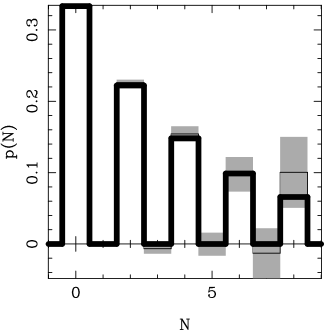
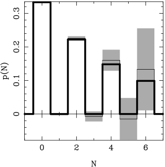
Figure 5.2: Probability distribution for the total number of photons of the twin beams in Eq. (5.21) for average number of photons per beam $\overline{n}=2$ obtained using the estimator in Eq. (5.17). The oscillation of the total photon-number probability due to the perfect correlation of the twin beams has been reconstructed by simulating $10^{7}$ data samples with quantum efficiency $\eta=0.9$ (on the left), and $2\times 10^{7}$ data samples $\eta=0.8$ (on the right). The theoretical probability (thick solid line) is superimposed onto the result of the Monte-Carlo experiment; the latter is shown by the thin solid line. Notice the dramatic increase of errors (in gray shade) versus N and for smaller $\eta$ (From Ref. [17]).

In Fig. 5.1 a Monte-Carlo simulation of the joint photon-number probability distribution is reported. The simulated values compare very well with the theoretical ones. In Ref. [17] a careful analysis of the statistical errors has been done for various twin-beam states by constructing histograms of deviations of the results from different simulated experiments from the theoretical ones. In comparison to the customary two-LO tomography of Ref. [87], where for $\eta=1$ the statistical errors saturate for increasingly large $n$ and $m$, here we have statistical errors that are slowly increasing versus $n$ and $m$. This is due to the fact that the range of the estimators in Eq. (5.16) increases versus $n$ and $m$. Overall we find that for any given quantum efficiency the statistical errors are generally slightly larger than those obtained with the two-LO method. The convenience of using a single LO then comes with its own price tag.

By using the estimator in Eq. (5.17) the probability distribution for the total number of photons $N$ of the twin beams has been also constructed (Fig. 5.2). Notice the dramatic increase of error bars versus N and for smaller $\eta$.

Figure 5.3: Tomographic reconstruction of the matrix elements $C_{n,m}\equiv{}_{a}\langle m|{}_{b}\langle m|\Psi\rangle\langle\Psi|n\rangle_{a}|n\rangle_{b}$ of the twin beams in Eq. (5.21) for average number of photons per beam $\overline{n}=2$, obtained using the estimator in Eq. (5.12). On the left we used $10^{6}$ simulated data samples and quantum efficiency $\eta=0.9$; on the right $3\times 10^{6}$ data samples and $\eta=0.8$. The coherence of the twin-beam state is easily recognized as $C_{n,m}$ varies little for $n+m=\mbox{constant}$ [$\xi$ in Eq. (5.21) has been chosen real]. For a typical comparison between theoretical and experimental matrix elements and their relative statistical errors, see results in Fig. 5.2 (From Ref. [17]).

Finally, in Fig. 5.3 we report the results of the tomographic measurement of $C_{n,m}$ defined in Eq. (5.39). Because the reconstructed $C_{n,m}$ is close to the theoretically expected value in Eq. (5.40), these reveal the purity of the twin beams, which cannot be inferred from the thermal diagonal distribution of Fig. 5.1.

The first experimental results of a measurement of the joint photon-number probability distribution for a two-mode quantum state created by a nondegenerate optical parametric amplifier has been presented in Ref. [86]. In this experiment, however, the twin beams are detected separately by two balanced-homodyne detectors. A schematic of the experimental setup is reported in Fig. 5.4, and some experimental results are reported in Fig. 5.5. As expected for parametric fluorescence, the experiment has shown a measured joint photon-number probability distribution that exhibited up to 1.9 dB of quantum correlation between the two modes, with thermal marginal distributions.

Figure 5.4: A schematic of the experimental setup. NOPA: non-degenerate optical parametric amplifier; LOs: local oscillators; PBS: polarizing beam splitter; LPFs: low-pass filters; BPF: band-pass filter; G: electronic amplifier. Electronics in the two channels are identical (From Ref. [86]).

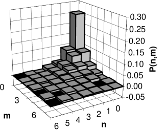
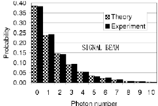
Figure 5.5: Left: Measured joint photon-number probability distribution for the twin-beam state with average number of photons per beam $\bar{n}=1.5$ and $400000$ samples. Right: marginal distribution for the signal beam for the same data. The theoretical distribution is also shown. Very similar results are obtained for the idler beam (From Ref. [86]).

Chapter 6 Applications to quantum measurements

In this chapter we review a number of applications of quantum tomography related to some fundamental tests in quantum mechanics.

First, we report the proposal of Ref. [30] for testing the nonclassicality of quantum states by means of an operational criterion based on a set of quantities that can be measured experimentally with some given level of confidence, even in the presence of loss, noise, and less-than-unity quantum efficiency.

Second, we report the experiment proposed in Ref. [31] for testing quantum state reduction. The state-reduction rule is tested using optical homodyne tomography by directly measuring the fidelity between the theoretically-expected reduced state and the experimental state.

Finally, we review some experimental results obtained at the Quantum Optics Lab of the University of Naples [32] about the reconstruction of coherent signals, together with application to the estimation of the losses introduced by simple optical components.

6.1 Measuring the nonclassicality of a quantum state

The concept of nonclassical states of light has drawn much attention in quantum optics [41, 88, 89, 90, 91, 92, 93, 94, 95, 96]. The customary definition of nonclassicality is given in terms of the $P$-function presented in Sec. 2.1: a nonclassical state does not admit a regular positive $P$-function representation, namely, it cannot be written as a statistical mixture of coherent states. Such states produce effects that have no classical analogue. These kinds of states are of fundamental relevance not only for the demonstration of the inadequacy of classical description, but also for applications, e.g., in the realms of information transmission and interferometric measurements [91, 92, 95].

We are interested in testing the nonclassicality of a quantum state by means of a set of quantities that can be measured experimentally with some given level of confidence, even in the presence of loss, noise, and less-than-unity quantum efficiency. The positivity of the $P$-function itself cannot be adopted as a test, since there is no viable method to measure it. As proved in Sec. 4.1 only the generalized Wigner functions of order $s<1-\eta^{-1}$ can be measured, $\eta$ being the quantum efficiency of homodyne detection. Hence, through this technique, all functions from $s=1$ to $s=0$ cannot be recovered, i.e., we cannot obtain the $P$-function and all its smoothed convolutions up to the customary Wigner function. For the same reason, the nonclassicality parameter proposed by Lee [41], namely, the maximum $s$-parameter that provides a positive distribution, cannot be experimentally measured.

Among the many manifestations of nonclassical effects, one finds squeezing, antibunching, even-odd oscillations in the photon-number probability, and negativity of the Wigner function [89, 90, 91, 95, 97, 98, 99, 100]. Any of these features alone, however, does not represent the univocal criterion we are looking for. Neither squeezing nor antibunching provides a necessary condition for nonclassicality [93]. The negativity of the Wigner function, which is well exhibited by the Fock states and the Schrödinger-cat-like states, is absent for the squeezed states. As for the oscillations in the photon-number probability, some even-odd oscillations can be simply obtained by using a statistical mixture of coherent states.

Many authors [93, 94, 96] have adopted the non-positivity of the phase-averaged $P$-function $F(I)={\frac{1}{2\pi}}\int_{0}^{2\pi}d\phi\,P(I^{1/2}e^{i\phi})$ as the definition for a nonclassical state, since $F(I)<0$ invalidates Mandel’s semiclassical formula [88] of photon counting, i.e., it does not allow a classical description in terms of a stochastic intensity. Of course, some states can exhibit a “weak” nonclassicality [96], namely, a positive $F(I)$, but with a non-positive $P$-function (a relevant example being a coherent state undergoing Kerr-type self-phase modulation). However, from the point of view of the detection theory, such “weak” nonclassical states still admit a classical description in terms of positive intensity probability $F(I)>0$. For this reason, we adopt non-positivity of $F(I)$ as the definition of nonclassicality.

6.1.1 Single-mode nonclassicality

The authors of Refs. [93, 94, 96] have pointed out some relations between $F(I)$ and generalized moments of the photon distribution, which, in turn, can be used to test the nonclassicality. The problem is reduced to an infinite set of inequalities that provide both necessary and sufficient conditions for nonclassicality [94]. In terms of the photon-number probability $p(n)=\langle n|\rho|n\rangle$ of the state with density matrix $\rho$, the simplest sufficient condition involves the following three-point relation [94, 96]

$$B(n)\equiv(n+2)p(n)p(n+2)-(n+1)[p(n+1)]^{2}<0\;.$$ (6.1)

Higher-order sufficient conditions involve five-, seven-, …, $(2k+1)$-point relations, always for adjacent values of $n$. It is sufficient that just one of these inequalities is satisfied in order to assure the negativity of $F(I)$. Notice that for a coherent state $B(n)=0$ identically for all $n$.

In the following we show that quantum tomography can be used as a powerful tool for performing the nonclassicality test in Eq. (6.1). For less-than-unity quantum efficiency ($\eta<1$), we rely on the concept of a “noisy state” $\rho_{\eta}$, wherein the effect of quantum efficiency is ascribed to the quantum state itself rather than to the detector. In this model, the effect of quantum efficiency is treated in a Schrödinger-like picture, with the state evolving from $\rho$ to $\rho_{\eta}$, and with $\eta$ playing the role of a time parameter. Such lossy evolution is described by the master equation [37]

$$\partial_{t}\rho(t)={\frac{\Gamma}{2}}\left[2a\rho(t)a^{{\dagger}}-a^{{\dagger}}a\rho(t)-\rho(t)a^{{\dagger}}a\right]\;,$$ (6.2)

wherein $\rho(t)\equiv\rho_{\eta}$ with $t=-\ln\eta/\Gamma$.

For the nonclassicality test, reconstruction in terms of the noisy state has many advantages. In fact, for non-unit quantum efficiency $\eta<1$ the tomographic method introduces errors for $p(n)$ which are increasingly large versus $n$, with the additional limitation that quantum efficiency must be greater than the minimum value $\eta=0.5$. On the other hand, the reconstruction of the noisy-state probabilities $p_{\eta}(n)=\langle n|\rho_{\eta}|n\rangle$ does not suffer such limitations, and even though all quantum features are certainly diminished in the noisy-state description, nevertheless the effect of non-unity quantum efficiency does not change the sign of the $P$-function, but only rescales it as follows:

$$P(z)\rightarrow P_{\eta}(z)={\frac{1}{\eta}}P(z/\eta^{1/2})\;.$$ (6.3)

Hence, the inequality (6.1) still represents a sufficient condition for nonclassicality when the probabilities $p(n)=\langle n|\rho|n\rangle$ are replaced with $p_{\eta}(n)=\langle n|\rho_{\eta}|n\rangle$, the latter being given by a Bernoulli convolution, as shown in Eq. (2.27). When referred to the noisy-state probabilities $p_{\eta}(n)$, the inequality in Eq. (6.1) keeps its form and simply rewrites as follows

$$B_{\eta}(n)\equiv(n+2)p_{\eta}(n)p_{\eta}(n+2)-(n+1)[p_{\eta}(n+1)]^{2}<0\;.$$ (6.4)

The quantities $B(n)$ and $B_{\eta}(n)$ are nonlinear in the density matrix. Then, they cannot be measured by averaging a suitable estimator over the homodyne data. Hence, in the evaluation of $B(n)$ one has to reconstruct the photon-number probabilities $p(n)$, using the estimator ${\cal R}_{\eta}[|n\rangle\langle n|](x,\varphi)$ in Eq. (3.44). The noisy-state probabilities $p_{\eta}(n)$ are obtained by using the same estimator for $\eta=1$, namely without recovering the convolution effect of non-unit quantum efficiency. Notice that the estimator does not depend on the phase of the quadrature. Hence, the knowledge of the phase of the local oscillator in the homodyne detector is not needed for the tomographic reconstruction, and it can be left fluctuating in a real experiment.

Regarding the estimation of statistical errors, they are generally obtained by dividing the set of homodyne data into blocks, as shown in Sec. 3.3.1. However, in the present case, the nonlinear dependence on the photon number probability introduces a systematic error that is vanishingly small for increasingly larger sets of data. Therefore, the estimated value of $B(n)$ is obtained from the full set of data, instead of averaging the mean value of the different statistical blocks.

Figure 6.1: Tomographic measurement of $B(n)$ (dashed trace) with the respective error bars (superimposed in gray-shade) along with the theoretical values (solid trace) for a Schrödinger cat state with average photon number $\bar{n}=5$ (left); for a phase-squeezed state with $\bar{n}=5$ and $\bar{n}_{\rm sq}=\sinh^{2}r=3$ squeezing photons (right). In both cases the quantum efficiency is $\eta=0.8$ and the number of simulated experimental data is $10^{7}$ (From Ref. [30]).

In Figs. 6.1–6.2 some numerical results from Ref. [30] are reported, which are obtained by a Monte-Carlo simulation of a quantum tomography experiment. The nonclassicality criterion is tested either on a Schrödinger-cat state $|\psi(\alpha)\rangle\propto(|\alpha\rangle+|-\alpha\rangle)$ or on a squeezed state $|\alpha,r\rangle\equiv D(\alpha)S(r)|0\rangle$, wherein $|\alpha\rangle$, $D(\alpha)$, and $S(r)$ denote a coherent state with amplitude $\alpha$, the displacement operator $D(\alpha)=e^{\alpha a^{{\dagger}}-\alpha^{*}a}$, and the squeezing operator $S(r)=e^{r(a^{{\dagger}2}-a^{2})/2}$, respectively. Fig. 6.1 shows tomographically-obtained values of $B(n)$, with the respective error bars superimposed, along with the theoretical values for a Schrödinger-cat state and for a phase-squeezed state ($r>0$). For the same set of states the results for $B_{\eta}(n)$ obtained by tomographic reconstruction of the noisy state are reported in Fig. 6.2. Let us compare the statistical errors that affect the of $B(n)$ and $B_{\eta}(n)$ on the original and the noisy states, respectively. In the first case the error increases with $n$, whereas in the second it remains nearly constant, albeit with less marked oscillations in $B_{\eta}(n)$ than those in $B(n)$.

Figure 6.2: Same as Fig. 6.1, but here for $B_{\eta}(n)$ (From Ref. [30]).

The nonclassicality of the states here analyzed is experimentally verifiable, as $B_{\eta}(0)<0$ by more than five standard deviations. In contrast, for coherent states one obtains small statistical fluctuations around zero for all $n$. Finally, we remark that the simpler test of checking for antibunching or oscillations in the photon-number probability in the case of the phase-squeezed state (left of Figs. 6.1 and 6.2) would not reveal the nonclassical features of such a state.

6.1.2 Two-mode nonclassicality

In Ref. [30] it is also shown how quantum homodyne tomography can also be employed to test the nonclassicality of two-mode states. For a two-mode state nonclassicality is defined in terms of non-positivity of the following phase-averaged two-mode $P$-function [96]:

$$F(I_{1},I_{2},\phi)=\frac{1}{2\pi}\int_{0}^{2\pi}d\phi_{1}\,P(I_{1}^{1/2}e^{i\phi_{1}},I_{2}^{1/2}e^{i(\phi_{1}+\phi)})\;.$$ (6.5)

In Ref. [96] it is also proved that a sufficient condition for nonclassicality is

$$C=\langle(n_{1}-n_{2})^{2}\rangle-(\langle n_{1}-n_{2}\rangle)^{2}-\langle n_{1}+n_{2}\rangle<0\;,$$ (6.6)

where $n_{1}$ and $n_{2}$ are the photon-number operators of the two modes.

A tomographic test of the inequality in Eq. (6.6) can be performed by averaging the estimators for the involved operators using Table 4.1. Again, the value $\eta=1$ can be used to reconstruct the ensemble averages of the noisy state $\rho_{\eta}$. As an example, we consider the twin-beam state of Eq. (5.21). The theoretical value of $C$ is given by $C=-2|\xi|^{2}/(1-|\xi|^{2})<0$. With regard to the effect of quantum efficiency $\eta<1$, the same argument still holds as for the single-mode case: one can evaluate $C_{\eta}$ for the twin beams degraded by the effect of loss, and use $\eta=1$ in the estimators. In this case, the theoretical value of $C_{\eta}$ is simply rescaled, namely

$$C_{\eta}=-2\eta^{2}|\xi|^{2}/(1-|\xi|^{2})\;.$$ (6.7)

In Fig. 6.3 we report $C_{\eta}$ vs. $1-\eta$, with $\eta$ ranging from 1 to 0.3 in steps of 0.05, for the twin beam in Eq. (5.21) with $|\xi|^{2}=0.5$, corresponding to a total average photon number $\langle n_{1}+n_{2}\rangle=2$. The values of $C_{\eta}$ result from a Monte-Carlo simulation of a homodyne tomography experiment with a sample of $4\times 10^{5}$ data. The nonclassicality test in terms of the noisy state gives values of $C_{\eta}$ that are increasingly near the classically positive region for decreasing quantum efficiency $\eta$. However, the statistical error remains constant and is sufficiently small to allow recognition of the nonclassicality of the twin beams up to $\eta=0.3$.

Figure 6.3: Tomographic measurement of the nonclassical parameter $C_{\eta}$ for twin beams in Eq. (5.21) with $|\xi|^{2}=0.5$. The results are shown for different values of the quantum efficiency $\eta$ (in steps of 0.05), and for each value the number of simulated data is $4\times 10^{5}$. Statistical errors are shown in the gray shade (From Ref. [30]).

We conclude that quantum homodyne tomography allows one to perform nonclassicality tests for single- and two-mode radiation states, even when the quantum efficiency of homodyne detection is rather low. The method involves reconstruction of the photon-number probability or of some suitable function of the number operators pertaining to the noisy state, namely, the state degraded by the less-than-unity quantum efficiency. The noisy-state reconstruction is affected by the statistical errors; however, they are sufficiently small that the nonclassicality of the state can be tested even for low values of $\eta$. For the cases considered here, we have shown that the nonclassicality of the states can be proved (deviation from classicality by many error bars) with $10^{5}$–$10^{7}$ homodyne data. Moreover, since the knowledge of the phase of the local oscillator in the homodyne detector is not needed for the tomographic reconstruction, it can be left fluctuating in a real experiment.

6.2 Test of state reduction

In quantum mechanics the state reduction (SR) is still a very discussed rule. The so–called “projection postulate” was introduced by von Neumann [2] to explain the results from the Compton-Simons experiment, and it was generalized by Lüders [101] for measurements of observables with degenerate spectrum. The consistency of the derivation of the SR rule and its validity for generic measurements have been analyzed with some criticism [102]. In a very general context, the SR rule was derived in a physically consistent way from the Schrödinger equation for the composite system of object and measuring apparatus [103]. An experiment for testing quantum SR is therefore a very interesting matter. Such a test in general is not equivalent to a test of the repeatability hypothesis since the latter holds only for measurements of observables that are described by self-adjoint operators. For example, joint measurements like the Arthurs-Kelly [54] are not repeatable, as the reduced states are coherent states, which are not orthogonal.

Quantum optics offers a possibility of testing the SR, because several observables can be chosen to perform different measurements on a fixed system. For instance, one can decide to perform either homodyne or heterodyne, or photon-number detection. This is a unique opportunity; in contrast, in particle physics the measurements are mostly quasi-classical and restricted to only a few observables. In addition, optical homodyne tomography allows a precise determination of the quantum system after the SR.

A scheme for testing the SR could be based on tomographic measurements of the radiation density matrix after nondemolition measurements. However, such a scheme would reduce the number of observables that are available for the test. Instead, one can take advantage of the correlations between the twin beams of Eq. (5.21) produced by a non-degenerate optical parametric amplifier (NOPA), in which case one can test the SR even for demolitive-type measurements. Indeed, if a measurement is performed on one of the twin beams, the SR can be tested by homodyne tomography on the other beam. This is precisely the scheme for an experimental test of SR proposed in Ref. [31], which is reviewed in the following.

The scheme for the SR test is given in Fig. 6.4. Different kinds of measurements can be performed on beam 1, even though here the SR only for heterodyne detection and photon-number detection will be considered.

Figure 6.4: Schematic of the proposed scheme for testing the SR for heterodyne detection. A NOPA generates a pair of twin beams (1 and 2). After heterodyning beam 1, the reduced state of beam 2 is analyzed by homodyne tomography, which is conditioned by the heterodyne outcome. In place of the heterodyne detector one can put any other kind of detector for testing the SR on different observables. We also consider the case of direct photodetection (From Ref.[31]).

For a system described by a density operator $\rho$, the probability $p(\lambda)d\lambda$ that the outcome of a quantum measurement of an observable is in the interval $[\lambda,\lambda+d\lambda)$ is given by Born’s rule $p(\lambda)d\lambda=\mbox{Tr}[\rho\,\Pi_{\lambda}d\lambda]$, where $\Pi_{\lambda}$ is the POVM pertaining to the measurement that satisfies $\Pi_{\lambda}\geq 0$ and $\int d\lambda\,\Pi_{\lambda}=I$. For an exact measurement of an observable, which is described by a self-adjoint operator, $\Pi_{\lambda}$ is just the projector over the eigenvector corresponding to the outcome $\lambda$. In the case of the photon number $a^{\dagger}a$ the spectrum is discrete and the POVM is $\Pi_{m}=|m\rangle\langle m|$ for integer eigenvalue $m$. For the Arthurs-Kelly joint measurement of the position and momentum (corresponding to a joint measurement of two conjugated quadratures of the field) we have the coherent-state POVM $\Pi_{\alpha}=\pi^{-1}|\alpha\rangle\langle\alpha|$.

When on beam 1 we perform a measurement described by $\Pi_{\lambda}$, the reduced normalized state of beam 2 is

$$\rho(\lambda)=\frac{\mbox{Tr}_{1}[|\xi\rangle\langle\xi|(\Pi_{\lambda}\otimes 1)]}{\mbox{Tr}_{1,2}[|\xi\rangle\langle\xi|(\Pi_{\lambda}\otimes 1)]}=\frac{\Xi\Pi^{\tau}_{\lambda}\Xi^{\dagger}}{p(\lambda)}\,,$$ (6.8)

where $O^{\tau}$ denotes the transposed operator (on a fixed basis), $\Xi=(1-|\xi|^{2})^{1/2}\xi^{a^{\dagger}a}$, and $p(\lambda)=\mbox{Tr}_{1,2}[\Xi\Pi^{\tau}_{\lambda}\Xi^{\dagger}]$ is the probability density of the measurement outcome $\lambda$. In the limit of infinite gain $|\xi|\to 1$ one has $\rho(\lambda)\propto\Pi_{\lambda}^{\tau}$. For example, for heterodyne detection with outcome $\alpha$, we have $\rho(\alpha)=|\alpha^{*}\rangle\langle\alpha^{*}|$.

If the readout detector on beam 1 has quantum efficiency $\eta_{r}$, Eq. (6.8) is replaced with

$$\rho^{\eta_{r}}(\lambda)=\frac{\Xi(\Pi_{\lambda}^{\eta_{r}})^{\tau}\Xi^{\dagger}}{p^{\eta_{r}}(\lambda)}\,,$$ (6.9)

where $p^{\eta_{r}}(\lambda)=\mbox{Tr}_{1,2}[\Xi(\Pi_{\lambda}^{\eta_{r}})^{\tau}\Xi^{\dagger}]$, and $\Pi_{\lambda}^{\eta_{r}}$ is the POVM for measurement with quantum efficiency $\eta_{r}$. As shown in Sec. 2.4, for heterodyne detection one has the Gaussian convolution

$$\Pi_{\alpha}^{\eta_{r}}=\frac{1}{\pi}\int_{\mathbb{C}}\frac{d^{2}z}{\pi\Delta_{\eta_{r}}^{2}}\,e^{-\frac{|z-\alpha|^{2}}{\Delta_{r}^{2}}}|z\rangle\langle z|\,,$$ (6.10)

with $\Delta_{\eta_{r}}^{2}=(1-\eta_{r})/\eta_{r}$. For direct photodetection $\Pi_{m}=|m\rangle\langle m|$ is replaced with the Bernoulli convolution

$$\Pi_{m}^{\eta_{r}}=\sum_{j=m}^{\infty}\left(\begin{array}[]{c}j\\ m\end{array}\right)\eta_{r}^{m}(1-\eta_{r})^{j-m}|j\rangle\langle j|\;.$$ (6.11)

The experimental test proposed here consists of performing conditional homodyne tomography on beam 2, given the outcome $\lambda$ of the measurement on beam 1. We can directly measure the “fidelity of the test”

$$F(\lambda)=\mbox{Tr}[\rho^{\eta_{r}}(\lambda)\,\rho_{\rm meas}(\lambda)]\,,$$ (6.12)

where $\rho^{\eta_{r}}(\lambda)$ is the theoretical state in Eq. (6.9), and $\rho_{\rm meas}(\lambda)$ is the experimentally measured state on beam 2. Notice that we use the term “fidelity” even if $F(\lambda)$ is a proper fidelity when at least one of the two states is pure, which occurs in the limit of unit quantum efficiency $\eta_{r}$. In the following we evaluate the theoretical value of $F(\lambda)$ and compare it with the tomographic measured value.

The fidelity (6.12) can be directly measured by homodyne tomography using the estimator for the operator $\rho^{\eta_{r}}(\lambda)$, namely

$$F(\lambda)=\int^{\pi}_{0}\frac{\mbox{d}\varphi}{\pi}\int^{+\infty}_{-\infty}dx\,p_{\eta_{h}}(x,\varphi;\lambda){\cal R}_{\eta_{h}}[\rho^{\eta_{r}}(\lambda)](x,\varphi)\;,$$ (6.13)

where $p_{\eta_{h}}(x,\varphi;\lambda)$ is the conditional homodyne probability distribution for outcome $\lambda$ at the readout detector.

For heterodyne detection on beam 1 with outcome $\alpha\in\mathbb{C}$, the reduced state on beam 2 is given by the displaced thermal state

$$\rho^{\eta_{r}}(\alpha)=\eta_{\xi}D(\gamma)(1-\eta_{\xi})^{a^{\dagger}a}D^{\dagger}(\gamma)\,,$$ (6.14)

where

$$\eta_{\xi}=1+(\eta_{r}-1)|\xi|^{2}\,,\qquad\gamma=\frac{\xi\eta_{r}}{\eta_{\xi}}\alpha^{*}\,.$$ (6.15)

The estimator in Eq. (6.13) is given by

$${\cal R}_{\eta_{h}}[\rho^{\eta_{r}}(\alpha)](x,\varphi)=\frac{2\eta_{h}\eta_{\xi}}{2\eta_{h}-\eta_{\xi}}\Phi\left(1,{\frac{1}{2}};-\frac{2\eta_{h}\eta_{\xi}}{2\eta_{h}-\eta_{\xi}}(x-\gamma_{\varphi})^{2}\right)\;,$$ (6.16)

where ${\gamma}_{\varphi}=\mbox{Re}({\gamma}e^{-i\varphi})$, and $\Phi(a,b;z)$ denotes the customary confluent hypergeometric function. The estimator in Eq. (6.16) is bounded for $\eta_{h}>{\frac{1}{2}}\eta_{\xi}$, then one needs to have

$$\eta_{h}>\frac{1}{2}\left[1-{|\xi|^{2}}(1-\eta_{r})\right]\,.$$ (6.17)

As one can see from Eq. (6.17), for $\eta_{h}>0.5$ the fidelity can be measured for any value of $\eta_{r}$ and any gain parameter $\xi$ of the NOPA. We recall that the condition $\eta_{h}>0.5$ is required for the measurement of the density matrix. However, in this direct measurement of the fidelity, the reconstruction of the density matrix is bypassed, and we see from Eq. (6.17) that the bound $\eta_{h}=0.5$ can be lowered.

The measured fidelity $F(\alpha)$ in Eq. (6.13) with $\rho^{\eta_{r}}(\alpha)$ as given in Eq. (6.14) must be compared with the theoretical value

$$F_{\rm th}=\eta_{\xi}/(2-\eta_{\xi})\;,$$ (6.18)

that is independent of $\alpha$.

For direct photodetection on beam 1 with outcome $n$, the reduced state on beam 2 is given by

$$\rho^{\eta_{r}}(n)=\eta_{\xi}\left(\frac{\eta_{\xi}}{1-\eta_{\xi}}\right)^{n}\left(\begin{array}[]{c}a^{{\dagger}}a\\ n\end{array}\right)(1-\eta_{\xi})^{a^{{\dagger}}a}\,.$$ (6.21)

The estimator for the fidelity measurement is

$${\cal R}_{\eta_{h}}[\rho^{\eta_{r}}(n)](x,\varphi)=\left.\frac{(\eta_{\xi}\partial_{z})^{n}}{n!}\right|_{z=0}\frac{2\eta_{h}\eta_{\xi}}{2\eta_{h}-\eta_{\xi}+z}\Phi\left(1,{\frac{1}{2}};-\frac{2\eta_{h}(\eta_{\xi}-z)}{2\eta_{h}-\eta_{\xi}+z}x^{2}\right)\,.$$ (6.22)

We see that the same bound of Eq. (6.17) holds. In this case the measured fidelity $F(n)$ must be compared with the theoretical value

$$F_{\rm th}(n)=\eta_{\xi}^{2+2n}F\left(2n+1,2n+1;1;(1-\eta_{\xi})^{2}\right)\,,$$ (6.23)

where $F(a,b;c;z)$ denotes the customary hypergeometric function.

Several simulations have been reported in Ref. [31] for both heterodyne and photodetection on beam 1. In the former case the quadrature probability distribution has been simulated, pertaining to the reduced state (6.14) on beam 2, and averaged the estimators in Eq. (6.16). In the latter case the reduced state (6.21) and the estimators in Eq. (6.22) have been used.

Numerical results for the fidelity was thus obtained for different values of the quantum efficiencies $\eta_{r}$ and $\eta_{h}$, and of the NOPA gain parameter $\xi$. A decisive test can be performed with samples of just a few thousand measurements. The statistical error in the measurement was found rather insensitive to both quantum efficiencies and NOPA gain.

6.3 Tomography of coherent signals and applications

Quantum homodyne tomography has been proved useful in various experimental situations, such as for measuring the photon statistics of a semiconductor laser [10], for determining the density matrix of a squeezed vacuum [11] and the joint photon-number probability distribution of a twin beam created by a non-degenerate optical parametric amplifier [86], and, finally, for reconstructing the quantum states of spatial modes with an array detector [104]. In this section we review some experimental results about homodyne tomography with coherent states, with application to the estimation of the loss introduced by simple optical components [32].

The experiment has been performed in the Quantum Optics Lab of the University of Naples, and its the schematic is presented in Fig. 6.5. The principal radiation source is provided by a monolithic Nd:YAG laser ($\approx$ 50 mW at 1064 nm; Lightwave, model 142). The laser has a linewidth of less than 10 kHz/ms with a frequency jitter of less than 300 kHz/s, while its intensity spectrum is shot–noise limited above 2.5 MHz.

Figure 6.5: Schematic of the experimental set-up. A Nd:YAG laser beam is divided into two beams, the first acting as a strong local oscillator, the second representing the signal beam. The signal is modulated at frequency $\Omega$ with a defined modulation depth to control the average photon number in the generated coherent state. The tomographic data are collected by a homodyne detector whose difference photocurrent is demodulated and then acquired by a digital oscilloscope (From Ref. [32]).

The laser emits a linearly polarized beam in a TEM00 mode, which is split in two parts by a beam splitter. One part provides the strong local oscillator for the homodyne detector. The other part, typically less than 200 $\mu$W, is the homodyne signal. The optical paths traveled by the local oscillator and the signal beams are carefully adjusted to obtain a visibility typically above $75\%$ measured at one of the homodyne output port. The signal beam is modulated, by means of a phase electro–optic modulator (EOM, Linos Photonics PM0202), at 4MHz, and a halfwave plate (HWP₂, HWP₃) is mounted in each path to carefully match the polarization state at the homodyne input.

The detector is composed by a 50$\div$50 beam splitter (BS), two amplified photodiodes (PD1, PD2), and a power combiner. The difference photocurrent is demodulated at 4MHz by means of an electrical mixer. In this way the detection occurs outside any technical noise and, more important, in a spectral region where the laser does not carry excess noise.

The phase modulation added to the signal beam moves a certain number of photons, proportional to the square of the modulation depth, from the carrier optical frequency $\omega$ to the side bands at $\omega\pm\Omega$ so generating two weak coherent states with engineered average photon number at frequencies $\omega\pm\Omega$. The sum sideband modes is then detected as a controlled perturbation attached to the signal beam. The demodulated current is acquired by a digital oscilloscope (Tektronix TDS 520D) with 8 bit resolution and record length of 250000 points per run. The acquisition is triggered by a triangular shaped waveform applied to the PZT mounted on the local oscillator path. The piezo ramp is adjusted to obtain a $2\pi$ phase variation between the local oscillator and the signal beam in an acquisition window.

The homodyne data to be used for tomographic reconstruction of the state have been calibrated according to the noise of the vacuum state. This is obtained by acquiring a set of data leaving the signal beam undisturbed while scanning the local oscillator phase. It is important to note that in case of the vacuum state no role is played by the visibility at the homodyne beam–splitter.

The tomographic samples consist of $N$ homodyne data $\{x_{j},\varphi_{j}\}_{j=1,...,N}$ with phases $\varphi_{j}$ equally spaced with respect to the local oscillator. Since the piezo ramp is active during the whole acquisition time, we have a single value $x_{j}$ for any phase $\varphi_{j}$. From calibrated data we first reconstruct the quantum state of the homodyne signal. According to the experimental setup, we expect a coherent signal with nominal amplitude that can be adjusted by varying the modulation depth of the optical mixer. However, since we do not compensate for the quantum efficiency of photodiodes in the homodyne detector ($\eta\simeq 90\%$) we expect to reveal coherent signals with reduced amplitude. In addition, the amplitude is further reduced by the non-maximum visibility (ranging from $75\%$ to $85\%$) at the homodyne beam–splitter.

In Fig. 6.6 we report a typical reconstruction, together with the reconstruction of the vacuum state used for calibration. For both states, we report the raw data, the photon number distribution $\rho_{nn}$, and a contour plot of the Wigner function. The matrix elements are obtained by sampling the corresponding estimators in Eq. (3.44), whereas the confidence intervals for diagonal elements are given by $\delta\rho_{nn}=\Delta\rho/\sqrt{N}$, $\Delta\rho$ being the rms deviation of the estimator over data. For off-diagonal elements the confidence intervals are evaluated for the real and imaginary part separately.

In order to see the quantum state as a whole, we also report the reconstruction of the Wigner function of the field, which can be expressed in terms of the matrix elements as the discrete Fourier transform

$$W(\alpha,\alpha^{*})=\mbox{Re}\sum_{d=0}^{\infty}e^{id\varphi}\sum_{n=0}^{\infty}\Lambda(n,d;|\alpha|)\rho_{n,n+d}\;$$ (6.24)

where $\varphi=\arg\alpha$, and

$$\Lambda(n,d;|\alpha|)=(-)^{n}2(2-\delta_{d0})|2\alpha|^{d}\sqrt{\frac{n!}{(n+d)!}}e^{-2|\alpha|^{2}}L_{n}^{d}(|2\alpha|^{2})\;,$$ (6.25)

$L_{n}^{d}(x)$ denoting the Laguerre polynomials. Of course, the series in Eq. (6.24) should be truncated at some point, and therefore the Wigner function can be reconstructed only at some finite resolution.

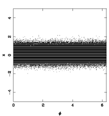
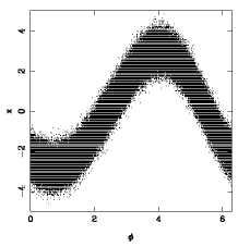
Figure 6.6: Reconstruction of the quantum state of the signal, and of the vacuum state used for calibration. For both states, from left to right, we report the raw data, a histogram of the photon number distribution, and a contour plot of the Wigner function. The reconstruction has been performed by a sample of $N=242250$ homodyne data. The coherent signal has an estimated average photon number equal to $\langle a^{\dagger}a\rangle=8.4$. The solid line denotes the theoretical photon distribution of a coherent state with such number of photons. Statistical errors on matrix elements are about $2\%$ . The slight phase asymmetry in the Wigner distribution corresponds to a value of about $2\%$ of the maximum (From Ref. [32]).

Once the coherence of the signal has been established we may use homodyne tomography to estimate the loss imposed by a passive optical component like an optical filter. The procedure may be outlined as follows. We first estimate the initial mean photon number $\bar{n}_{0}=|\alpha_{0}|^{2}$ of the signal beam, and then the same quantity inserting an optical neutral density filter in the signal path. If $\Gamma$ is the loss parameter, then the coherent amplitude is reduced to $\alpha_{\Gamma}=\alpha_{0}e^{-\Gamma}$, and the intensity to $\bar{n}_{\Gamma}=\bar{n}_{0}e^{-2\Gamma}$.

The estimation of the mean photon number can be performed adaptively on data, using the general method presented in Sec. 3.4.2. One takes the average of the estimator

$${\cal R}[a^{{\dagger}}a](x,\varphi)=2x^{2}-\frac{1}{2}+\mu e^{i2\varphi}+\mu^{*}e^{-i2\varphi}\;,$$ (6.26)

where $\mu$ is a parameter to be determined in order to minimize fluctuations. As proved in Ref. [22] one has $\mu=-1/2\langle a^{{\dagger}2}\rangle$, which itself can be obtained from homodyne data. In practice, one uses the data sample twice: first to evaluate $\mu$, then to obtain the estimate for the mean photon number.

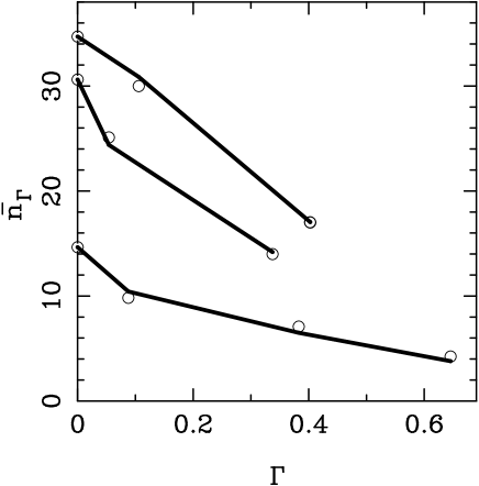
Figure 6.7: Estimation of the mean photon number of a coherent signal as a function of the loss imposed by an optical filter. Three set of experiments, corresponding to three different initial amplitudes are reported. Open circles are the tomographic determinations, whereas solid line denotes the expected values, as follow from nominal values of loss and visibility at homodyne detector. Statistical errors are within the circles (From Ref. [32]).

In Fig. 6.7 the tomographic determinations of $\bar{n}_{\Gamma}$ are compared with the expected values for three set of experiments, corresponding to three different initial amplitudes. The expected values are given by $\bar{n}_{\Gamma}=\bar{n}_{0}e^{-2\Gamma}{\cal V}$, where $\Gamma$ is the value obtained by comparing the signal dc currents $I_{0}$ and $I_{\Gamma}$ at the homodyne photodiodes and ${\cal V=V}_{\Gamma}/{\cal V}_{0}$ is the relative visibility. The solid line in Fig. 6.7 denotes these values. The line is not continuous due to variations of visibility. It is apparent from the plot that the estimation is reliable in the whole range of values we could explore. It is worth noting that the estimation is absolute, i.e. it does not depend on the knowledge of the initial amplitude, and it is robust, since it can be performed independently on the quantum efficiency of the homodyne detector.

One may notice that the estimation of loss can be pursued also by measuring an appropriate observable, typically the intensity of the light beam with and without the filter. However, this is a concrete possibility only for high amplitude signals, whereas losses on weak coherent states cannot be properly characterized neither by direct photocounting using photodiodes (due to the low quantum efficiency and large fluctuations), nor by avalanche photodetectors (due to the impossibility of discriminating among the number of photons). On the contrary, homodyne tomography provides the mean intensity (actually the whole photon distribution) independently on the signal level, thus allowing a precise characterization also in the quantum regime. Indeed, in Ref. [22] adaptive tomographic determination of the mean photon number has been extensively applied to (numerically simulated) homodyne data for coherent states of various amplitudes. The analysis has shown that the determination is reliable also for small samples and that precision is not much affected by the intensity of the signal.

Chapter 7 Tomography of a quantum device

If we want to determine experimentally the operation of a quantum device, we need, by definition, quantum tomography. In fact, the characterization of the device operation could be done by running a basis of possible known inputs, and determining the corresponding outputs by quantum tomography. In quantum mechanics the inputs are density operators, and the role of the transfer matrix is played by the so-called quantum operation of the device, here denoted by $\cal E$. Thus the output state $\rho_{out}$ (a part from a possible normalization) is given by the quantum operation applied to the input state as follows

$$\rho_{out}={\cal{E}}(\rho_{in}).$$ (7.1)

Since the set of states $\rho$ actually belongs to a space of operators, this means that if we want to characterize $\cal{E}$ completely, we need to run a complete orthogonal basis of quantum states $|n\rangle$ ($n=0,1,2,\ldots$), along with their linear combinations $\frac{1}{\sqrt{2}}(|n^{\prime}\rangle+i^{k}|n^{\prime\prime}\rangle)$, with $k=0,1,2,3$ and $i$ denoting the imaginary unit. However, the availability of such a set of states in the lab is, by itself, a very hard technological problem. For example, for an optical device, the states $|n\rangle$ are those with a precise number $n$ of photons, and, a part from very small $n$—say at most n=2—they have never been achieved in the lab, whereas preparing their superpositions remains a dream for experimentalists, especially if $n\gg 1$ (a kind of Schrődinger kitten states).

The idea of achieving the quantum operation of a device by scanning the inputs and making tomography of the corresponding output is the basis of the early methods proposed in Refs. [105, 106]. Due to the mentioned problems in the availability of input states, both methods have limited application. The method of Ref. [105] has been designed for NMR quantum processing, whereas the method of Ref. [106] was conceived for determining the Liouvillian of a phase-insensitive amplifier, namely for a case in which the quantum operation has no off-diagonal matrix elements, to evaluate which one needs the superpositions $\frac{1}{\sqrt{2}}(|n^{\prime}\rangle+i^{k}|n^{\prime\prime}\rangle)$ with $k=0,1,2,3$ mentioned above. The problem of availability of input spates and their superpositions was partially solved by the method of Ref. [107], where it was suggested to use randomly drawn coherent states to estimate the quantum operation of an optical device via a maximum likelihood approach. This method, however, cannot be used for quantum systems different from the em radiation—such as finite dimensional systems, i.e. qubits—due to the peculiarity of coherent states. The solution to the problem came with the recent method of Ref. [25], where the problem of the availability of input states was solved by using a single bipartite entangled input, which is equivalent to run all possible input states in a kind of “quantum parallel” fashion (bipartite entangled states are nowadays easily available in most quantum systems of interest). The method is also very simple and effective, and its experimental feasibility (for single-photon polarization-encoded qubits) has been already demonstrated in a recent experiment performed in the Francesco De Martini laboratory in Roma La Sapienza [108]. In the next sections we will review the general method and report some computer simulated results from Ref. [25].

7.1 The method

As already mentioned, the most description of a general state-transformation in quantum mechanics is given in terms of the so-called quantum operation. The state transformation due to the quantum operation ${\cal E}$ is given as follows

$$\rho\rightarrow\frac{{\cal E}(\rho)}{\mbox{Tr}\bigl{(}{\cal E}(\rho)\bigr{)}}.$$ (7.2)

The transformation occurs with probability given by $p=\hbox{Tr}[{\cal E}(\rho)]\leq 1$. The quantum operation ${\cal E}$ is a linear, trace-decreasing completely positive (CP) map. We remind that a map is completely positive if it preserves positivity generally when applied locally to an entangled state. In other words, upon denoting by ${\cal I}$ the identical map on the Hilbert space ${\cal K}$ of a second quantum system, the extended map ${\cal E}\otimes{\cal I}$ on ${\cal H}\otimes{\cal K}$ is positive for any extension ${\cal K}$. Typically, the CP map is written using a Kraus decomposition [109] as follows

$${\cal E}(\rho)=\sum_{n}K_{n}\rho K_{n}^{\dagger}\;,$$ (7.3)

where the operators $K_{n}$ satisfy

$$\sum_{n}K_{n}^{\dagger}K_{n}\leq I\;.$$ (7.4)

The transformation (7.3) occurs with generally non-unit probability $\hbox{Tr}[{\cal E}(\rho)]\leq 1$, and the probability is unit independently on $\rho$ when ${\cal E}$ is trace-preserving, i.e. when we have the equal sign in Eq. (7.4). The particular case of unitary transformations corresponds to having just one term $K_{1}=U$ in the sum (7.3), with $U$ unitary. However, one can consider also non-unitary operations with one term only, namely

$${\cal E}(\rho)=A\rho A^{\dagger}\;,$$ (7.5)

where $A$ is a contraction, i. e. $||A||\leq 1$. Such operations leave pure states as pure, and describes, for example, the state reduction from a measurement apparatus for a particular fixed outcome that occurs with probability $\mbox{Tr}[\rho A^{\dagger}A]\leq 1$.

In the following we will use the notation for bipartite pure states introduced in Eq. (2.60), and we will denote by $O^{\tau}$ and $O^{*}$ the transposed and the conjugate operator of $O$ with respect to some pre-chosen orthonormal basis.

The basic idea of the method in Ref. [25] is the following. An unknown quantum operation $\cal E$ can be determined experimentally through quantum tomography, by exploiting the following one-to-one correspondence ${\cal E}\leftrightarrow R_{{\cal E}}$ between quantum operations $\cal E$ and positive operators $R_{\cal E}$ on two copies of the Hilbert space ${\cal H}\otimes{\cal H}$

$$R_{{\cal E}}={\cal E}\otimes{\cal I}(|I{\rangle\!\rangle}{\langle\!\langle}I|),\qquad{\cal E}(\rho)=\hbox{Tr}_{2}[I\otimes{\rho^{\tau}}R_{\cal E}]\;.$$ (7.6)

Notice that the vector $|I{\rangle\!\rangle}$ represents a (unnormalized) maximally entangled state. If we consider a bipartite input state $|\psi{\rangle\!\rangle}$ and operate with $\cal E$ only on one Hilbert space as in Fig. 7.1, the output state is given by

$$R(\psi)\equiv{\cal E}\otimes{\cal I}(|\psi{\rangle\!\rangle}{\langle\!\langle}\psi|).$$ (7.7)

For invertible $\psi$ the two matrices $R(I)\equiv R_{\cal E}$ and $R(\psi)$ are related as follows

$$R(I)=(I\otimes{\psi^{-1}}^{\tau}R(\psi)(I\otimes\psi^{-1*})\;.$$ (7.8)

Hence, the (four-index) quantum operation matrix $R_{\cal E}$ can be obtained by estimating via quantum tomography the following ensemble averages

$${\langle\!\langle}i,j|R(I)|l,k{\rangle\!\rangle}=\hbox{Tr}\left[R(\psi)\left(|l\rangle\langle i|\otimes\psi^{-1*}|k\rangle\langle j|\psi^{-1*}\right)\right]\;.$$ (7.9)

Then one simply has to perform a quantum tomographic estimation, by measuring jointly two observables $X_{\lambda}$ and $X^{\prime}_{\lambda}$ from two quorums $\{X_{\lambda}\}$ and $\{X^{\prime}_{\lambda}\}$ for the two entangled quantum systems.

Figure 7.1: General scheme of the method for the tomographic estimation of a quantum operation. Two identical quantum systems are prepared in a bipartite state $|\psi\rangle\!\rangle$, with invertible $\psi$. One of the two systems undergoes the quantum operation $\cal E$, whereas the other is left untouched. At the output one performs a quantum tomographic estimation, by measuring jointly two observables $X_{\lambda}$ and $X^{\prime}_{\lambda}$ from two quorums $\{X_{\lambda}\}$ and $\{X^{\prime}_{\lambda}\}$ for the two Hilbert spaces, such as two different quadratures of the two field modes in a two-mode homodyne tomography (From Ref. [25]).

7.2 An example in the optical domain

In Ref. [25] it is shown that the proposed method for quantum tomography of a device can be actually performed using joint homodyne tomography on a twin-beam from downconversion of vacuum, with an experimental setup similar to that used in the experiment in Ref. [86]. The feasibility analysis considers, as an example, the experimental determination of the quantum operation corresponding to the unitary displacement operator $D(z)=e^{za^{{\dagger}}-z^{*}a}$. The pertaining matrix $R(I)$ is given by

$$R(I)=|D(z){\rangle\!\rangle}{\langle\!\langle}D(z)|\;,$$ (7.10)

which is the (unnormalizable) eigenstate of the operator $a-b^{\dagger}$ with eigenvalue $z$, as shown in Sec. 2.4. As an input bipartite state, one uses the twin-beam from parametric downconversion of Eq. (5.21), which is clearly invertible, since

$$\psi=\sqrt{1-|\xi|^{2}}\,\xi^{a^{\dagger}a}\;,\qquad\psi^{-1}=\frac{1}{\sqrt{1-|\xi|^{2})}}\,\xi^{-a^{\dagger}a}\;.$$ (7.11)

The experimental apparatus is the same as in the experiment of Ref. [86], where the twin-beam is provided by a non-degenerate optical parametric amplifier (a KTP crystal) pumped by the second harmonic of a Q-switched mode-locked Nd:YAG laser, which produces a 100-MHz train of 120-ps duration pulses at 1064 nm. The orthogonally polarized twin beams emitted by the KTP crystal (one of which is displaced of $D(z)$ by a nearly transparent beam splitter with a strong local oscillator) are separately detected by two balanced homodyne detectors that use two independent local oscillators derived from the same laser. This provides the joint tomography of quadratures $X_{\phi^{\prime}}\otimes X_{\phi^{\prime\prime}}$ needed for the reconstruction. The only experimental problem which still need to be addressed (even though is practically solvable) with respect to the original experiment of Ref. [86] is the control of the quadrature phases $\phi^{\prime}$ and $\phi^{\prime\prime}$ with respect to the LO, which in the original experiment were random.

In Fig. 7.2 the results of a simulated experiment are reported, for displacement parameter $z=1$, and for some typical values of the quantum efficiency $\eta$ at homodyne detectors and of the total average photon number $\bar{n}$ of the twin beam. The diagonal elements $A_{nn}=\langle n|D(z)|n\rangle=[\langle n|\langle n|R_{D(z)}|n\rangle n\rangle]^{1/2}$ are plotted for the displacement operator with $z=1$. The reconstructed values are shown by thin solid line on an extended abscissa range, with their respective error bars in gray shade, and compared to the theoretical probability (thick solid line). A good reconstruction of the matrix can be achieved in the given range with $\bar{n}\sim 1$, quantum efficiency as low as $\eta=0.7$, and $10^{6}\div 10^{7}$ data. The number of data can be decreased by a factor $100-1000$ using the tomographic max-likelihood techniques of Ref. [23], however at the expense of the complexity of the algorithm. Improving quantum efficiency and increasing the amplifier gain (toward a maximally entangled state) have the effect of making statistical errors smaller and more uniform versus the photon labels $n$ and $m$ of the matrix $A_{nm}$.

Figure 7.2: Homodyne tomography of the quantum operation corresponding to the unitary displacement operator $D(z)$, with $z=1$. The reconstructed diagonal elements $A_{nn}=\langle n|D(z)|n\rangle$ are shown (thin solid line on an extended abscissa range, with their respective error bars in gray shade), compared to the theoretical value (thick solid line). Similar results are obtained for off-diagonal terms. The reconstruction has been achieved using at the input the twin beam state of Eq. (5.21), with total average photon number $\bar{n}$ and quantum efficiency at homodyne detectors $\eta$. Left: $\bar{n}=5$, $\eta=0.9$, and $150$ blocks of $10^{4}$ data have been used. Right: $\bar{n}=3$, $\eta=0.7$, and $300$ blocks of $2\cdot 10^{5}$ data have been used (From Ref. [25]).

It is worth emphasizing that the quantum tomographic method of Ref. [25] for measuring the matrix of a quantum operation can be much improved by means of a max-likelihood strategy aimed at the estimation of some unknown parameters of the quantum operation. In this case, instead of obtaining the matrix elements of $R(I)$ from the ensemble averages in Eq. (7.9), one parametrizes $R(I)$ in terms of unknown quantities to be experimentally determined, and the likelihood is maximized for the set of experimental data at various randomly selected (tensor) quorum elements, keeping the same fixed bipartite input state. This method is especially useful for a very precise experimental comparison between the characteristics of a given device (e.g. the gain and loss of an active fiber) with those of a quantum standard reference.

Chapter 8 Maximum-likelihood method in quantum estimation

Quantum estimation of states, observables and parameters is, from very basic principles, matter of statistical inference from a population sampling, and the most comprehensive quantum estimation procedure is quantum tomography. As we have shown in Chapter 3, the expectation value of an operator is obtained by averaging an estimator over the experimental data of a “quorum” of observables. The method is very general and efficient, however, in the averaging procedure, we have fluctuations which result in relatively large statistical errors.

Another relevant strategy, the maximum-likelihood (ML) method, can be used for measuring unknown parameters of transformation on a given state [33], or for measuring the matrix elements of the density operator itself [23]. The ML strategy [110, 111] is an entirely different approach to quantum state measurement compared to the standard quantum-tomographic techniques. The ML procedure consists in finding the quantum state, or the value of the parameters, that are most likely to generate the observed data. This idea can be quantified and implemented using the concept of the likelihood functional.

As regards state estimation, the ML method estimates the quantum state as a whole. Such a procedure incorporates a priori knowledge about relations between elements of the density matrix. This guarantees positivity and normalization of matrix, with the result of a substantial reduction of statistical errors. Regarding the estimation of specific parameters, we notice that in many cases the resulting estimators are efficient, unbiased and consistent, thus providing a statistically reliable determination.

As we will show, by using the ML method only small samples of data are required for a precise determination. However, we want to emphasize that such method is not always the optimal solution of the tomographic problem, since it suffers from some major limitations. Besides being biased due to the Hilbert space truncation—even though the bias can be very small if, from other methods, we know where to truncate—it cannot be generalized to the estimation of any ensemble average, but just of a set of parameters from which the density matrix depends. In addition, for increasing number of parameters the method has exponential complexity.

In the following we will review the ML methods proposed in Refs. [23] and [33], by deriving the likelihood functional, and applying the ML method to the quantum state reconstruction, with examples for both radiation and spin systems, and, finally, considering the ML estimation for the relevant class of Gaussian states in quantum optics.

8.1 Maximum likelihood principle

Here we briefly review the theory of the maximum-likelihood (ML) estimation of a single parameter. The generalization to several parameters, as for example the elements of the density matrix, is straightforward. The only point that should be carefully analyzed is the parameterization of the multidimensional quantity to be estimated. In the next section the specific case of the density matrix will be discussed.

Let $p(x|\lambda)$ the probability density of a random variable $x$, conditioned to the value of the parameter $\lambda$. The form of $p$ is known, but the true value of $\lambda$ is unknown, and will be estimated from the result of a measurement of $x$. Let $x_{1},x_{2},...,x_{N}$ be a random sample of size $N$. The joint probability density of the independent random variable $x_{1},x_{2},...,x_{N}$ (the global probability of the sample) is given by

$${\cal L}(x_{1},x_{2},...,x_{N}|\lambda)=\Pi_{k=1}^{N}p(x_{k}|\lambda)\;,$$ (8.1)

and is called the likelihood function of the given data sample (hereafter we will suppress the dependence of ${\cal L}$ on the data). The maximum-likelihood estimator (MLE) of the parameter $\lambda$ is defined as the quantity $\lambda_{ml}\equiv\lambda_{ml}(\{x_{k}\})$ that maximizes ${\cal L}(\lambda)$ for variations of $\lambda$, namely $\lambda_{ml}$ is given by the solution of the equations

$$\frac{\partial{\cal L}(\lambda)}{\partial\lambda}=0\;;\quad\frac{\partial^{2}{\cal L}(\lambda)}{\partial\lambda^{2}}<0\;.$$ (8.2)

The first equation is equivalent to $\partial L/\partial\lambda=0$ where

$$L(\lambda)=\log{\cal L}(\lambda)=\sum_{k=1}^{N}\log p(x_{k}|\lambda)\;$$ (8.3)

is the so-called log-likelihood function.

In order to obtain a measure for the confidence interval in the determination of $\lambda_{ml}$ we consider the variance

$$\sigma^{2}_{\lambda}=\int\left[\prod_{k}dx_{k}\,p(x_{k}|\lambda)\right]\left[\lambda_{ml}(\{x_{k}\})-\lambda\right]^{2}\;.$$ (8.4)

In terms of the Fisher information

$$F=\int dx\left[\frac{\partial p(x|\lambda)}{\partial\lambda}\right]^{2}\frac{1}{p(x|\lambda)}\;,$$ (8.5)

it is easy to prove that

$$\sigma^{2}_{\lambda}\geq\frac{1}{NF}\;,$$ (8.6)

where $N$ is the number of measurements. The inequality in Eq. (8.6) is known as the Cramér-Rao bound [112] on the precision of the ML estimation. Notice that this bound holds for any functional form of the probability distribution $p(x|\lambda)$, provided that the Fisher information exists $\forall\lambda$ and $\partial_{\lambda}p(x|\lambda)$ exists $\forall x$. When an experiment has ”good statistics” (i.e. for a large enough data sample) the Cramér-Rao bound is saturated.

8.2 ML quantum state estimation

In this section we review the method of the maximum likelihood estimation of the quantum state of Ref. [23], focusing attention to the cases of homodyne and spin tomography.

We consider an experiment consisting of $N$ measurements performed on identically prepared copies of a given quantum system. Each measurement is described by a positive operator-valued measure (POVM). The outcome of the $i$th measurement corresponds to the realization of a specific element of the POVM used in the corresponding run, and we denote this element by $\Pi_{i}$. The likelihood is here a functional of the density matrix ${\cal L}({\rho})$ and is given by the product

$${\cal L}({\rho})=\prod_{i=1}^{N}\hbox{Tr}({\rho}\Pi_{i})\;,$$ (8.7)

which represents the probability of the observed data. The unknown element of the above expression, which we want to infer from data, is the density matrix describing the measured ensemble. The estimation strategy of the ML technique is to maximize the likelihood functional over the set of the density matrices. Several properties of the likelihood functional are easily found, if we restrict ourselves to finite dimensional Hilbert spaces. In this case, it can be easily proved that ${\cal L}({\rho})$ is a concave function defined on a convex and closed set of density matrices. Therefore, its maximum is achieved either on a single isolated point, or on a convex subset of density matrices. In the latter case, the experimental data are insufficient to provide a unique estimate for the density matrix using the ML strategy. On the other hand, the existence of a single maximum allows us to assign unambiguously the ML estimate for the density matrix.

The ML estimation of the quantum state, despite its elegant general formulation, results in a highly nontrivial constrained optimization problem, even if we resort to purely numerical means. The main difficulty lies in the appropriate parameterization of the set of all density matrices. The parameter space should be of the minimum dimension in order to preserve the maximum of the likelihood function as a single isolated point. Additionally, the expression of quantum expectation values in terms of this parameterization should enable fast evaluation of the likelihood function, as this step is performed many times in the course of numerical maximization.

For such purpose one introduces [23] a parameterization of the set of density matrices which provides an efficient algorithm for maximization of the likelihood function. We represent the density matrix in the form

$${\rho}={T}^{\dagger}{T}\;,$$ (8.8)

which automatically guarantees that ${\rho}$ is positive and Hermitian. The remaining condition of unit trace $\hbox{Tr}{\rho}=1$ will be taken into account using the method of Lagrange multipliers. In order to achieve the minimal parameterization, we assume that ${T}$ is a complex lower triangular matrix, with real elements on the diagonal. This form of ${T}$ is motivated by the Cholesky decomposition known in numerical analysis [113] for arbitrary non negative Hermitian matrix. For an $M$-dimensional Hilbert space, the number of real parameters in the matrix ${T}$ is $M+2M(M-1)/2=M^{2}$, which equals the number of independent real parameters for a Hermitian matrix. This confirms that such parameterization is minimal, up to the unit trace condition.

In numerical calculations, it is convenient to replace the likelihood functional by its natural logarithm, which of course does not change the location of the maximum. Thus the log-likelihood function subjected to numerical maximization is given by

$$L({T})=\sum_{i=1}^{N}\ln\hbox{Tr}({T}^{\dagger}{T}\Pi_{i})-\lambda\hbox{Tr}({T}^{\dagger}{T})\;,$$ (8.9)

where $\lambda$ is a Lagrange multiplier accounting for normalization of $\rho$. Writing $\rho$ in terms of its eigenvectors $|\psi_{\mu}\rangle$ as $\rho=\sum_{\mu}y_{\mu}^{2}|\psi_{\mu}\rangle\langle\psi_{\mu}|$, with real $y_{\mu}$, the maximum likelihood condition $\partial L/\partial y_{\nu}=0$ reads

$$\lambda y_{\nu}=\sum_{i=1}^{N}[y_{\nu}\langle\psi_{\nu}|\Pi_{i}|\psi_{\nu}\rangle/\hbox{Tr}(\rho\Pi_{i})]\;,$$ (8.10)

which, after multiplication by $y_{\nu}$ and summation over $\nu$, yields $\lambda=N$. The Lagrange multiplier then equals the total number of measurements $N$.

This formulation of the maximization problem allows one to apply standard numerical procedures for searching the maximum over the $M^{2}$ real parameters of the matrix ${T}$. The examples presented below use the downhill simplex method [114].

The first example is the ML estimation of a single-mode radiation field. The experimental apparatus used in this technique is the homodyne detector. According to Sec. 2.4 the homodyne measurement is described by the positive operator-valued measure

$${\cal H}(x;\varphi)=\sqrt{\frac{2\eta}{\pi(1-\eta)}}\exp\left[-\frac{2\eta}{1-\eta}(X_{\varphi}-x)^{2}\right]\;,$$ (8.11)

where $\eta$ is the detector efficiency, and $X_{\varphi}=(a^{\dagger}\,e^{i\varphi}+a\,e^{-i\varphi})/2$ is the quadrature operator at phase $\varphi$.

Figure 8.1: Reconstruction of the density matrix of a single-mode radiation field by the ML method. The plot shows the matrix elements of a coherent state (left) with $\langle a^{{\dagger}}a\rangle=1$ photon, and for a squeezed vacuum (right) with $\langle a^{{\dagger}}a\rangle=0.5$ photon. A sample of 50000 simulated homodyne data for quantum efficiency $\eta=80\%$ has been used (From Ref. [23]).

After $N$ measurements, we obtain a set of pairs $(x_{i};\varphi_{i})$, where $i=1,\ldots,N$. The log-likelihood functional is given by Eq. (8.9) with $\Pi_{i}\equiv{\cal H}(x_{i};\varphi_{i})$. Of course, for a light mode it is necessary to truncate the Hilbert space to a finite dimensional basis. We shall assume that the highest Fock state has $M-1$ photons, i.e. that the dimension of the truncated Hilbert space is $M$. For the expectation $\mbox{Tr}[{T}^{\dagger}{T}{\cal H}(x;\varphi)]$ it is necessary to use an expression which is explicitly positive, in order to protect the algorithm against occurrence of small negative numerical arguments of the logarithm function. A simple derivation yields

$$\mbox{Tr}[{T}^{\dagger}{T}{\cal H}(x;\varphi)]=\sqrt{\eta}\sum_{k=0}^{M-1}\sum_{j=0}^{k}\left|\sum_{n=0}^{k-j}\langle k|{T}|n+j\rangle B_{n+j,n}\langle n|\sqrt{\eta}x\rangle e^{in\varphi}\right|^{2}\;,$$ (8.12)

where

$$B_{n+j,n}=\left[{{n+j}\choose n}\eta^{n}(1-\eta)^{j}\right]^{1/2}\;,$$ (8.13)

and

$$\langle n|x\rangle=\left(\frac{2}{\pi}\right)^{1/4}\frac{1}{\sqrt{2^{n}n!}}H_{n}(\sqrt{2}\,x)\,\exp(-x^{2})\;$$ (8.14)

are the eigenstates of the harmonic oscillator in the position representation—$H_{n}(x)$ being the $n$th Hermite polynomial.

The ML technique can be applied to reconstruct the density matrix in the Fock basis from Monte Carlo simulated homodyne statistics. Fig. 8.1 depicts the matrix elements of the density operator as obtained for a coherent state and a squeezed vacuum, respectively. Remarkably, only 50000 homodyne data have been used for quantum efficiency $\eta=80\%$. We recall that in quantum homodyne tomography the statistical errors are known to grow rapidly with decreasing efficiency $\eta$ of the detector [29, 80]. In contrast, the elements of the density matrix reconstructed using the ML approach remain bounded, as the whole matrix must satisfy positivity and normalization constraints. This results in much smaller statistical errors. As a comparison one could see that the same precision of the reconstructions in Fig. 8.1 could be achieved using $10^{7}$–$10^{8}$ data samples with conventional quantum tomography. On the other hand, in order to find numerically the ML estimate we need to set a priori the cut-off parameter for the photon number, and its value is limited by increasing computation time.

Figure 8.2: ML reconstruction of the density matrix of a two-mode radiation field. On the left the matrix elements obtained for the state $|\Psi_{1}\rangle=(|00\rangle+|11\rangle)/\sqrt{2}$; on the right for $|\Psi_{2}\rangle=(|01\rangle+|10\rangle)/\sqrt{2}$. For $|\Psi_{1}\rangle$ we used 100000 simulated homodyne data and $\eta=80\%$; for $|\Psi_{2}\rangle$ we used 20000 data and $\eta=90\%$ (From Ref. [23]).

Another relevant example is the reconstruction of the quantum state of two-mode field using single-LO homodyning of Chapter 5. Here, the full joint density matrix can be measured by scanning the quadratures of all possible linear combinations of modes. For two modes the measured quadrature operator is given by

$$X(\theta,\psi_{0},\psi_{1})=\frac{1}{2}({a}e^{-i\psi_{0}}\cos\theta+{b}e^{-i\psi_{1}}\sin\theta+\mbox{h.c.})\;,$$ (8.15)

where $(\theta,\psi_{0},\psi_{1})\in S^{2}\times[0,2\pi]$, $S^{2}$ being the Poincaré sphere and one phase ranging between $0$ and $2\pi$. In each run these parameters are chosen randomly. The POVM describing the measurement is given by the right-hand side of Eq. (8.11), with $X_{\varphi}$ replaced by $X(\theta,\psi_{0},\psi_{1})$. An experiment for the two orthogonal states $|\Psi_{1}\rangle=(|00\rangle+|11\rangle)/\sqrt{2}$ and $|\Psi_{2}\rangle=(|01\rangle+|10\rangle)/\sqrt{2}$ has been simulated, in order to reconstruct the density matrix in the two-mode Fock basis using the ML technique. The results are reported in Fig. 8.2.

The ML procedure can also be applied for reconstructing the density matrix of spin systems. For example, let us consider $N$ repeated preparations of a pair of spin-1/2 particles. The particles are shared by two parties. In each run, the parties select randomly and independently from each other a direction along which they perform a spin measurement. The obtained result is described by the joint projection operator (spin coherent states [115]) ${\cal F}_{i}=|\Omega^{A}_{i},\Omega^{B}_{i}\rangle\langle\Omega^{A}_{i},\Omega^{B}_{i}|$, where $\Omega^{A}_{i}$ and $\Omega^{B}_{i}$ are the vectors on the Bloch sphere corresponding to the outcomes of the $i$th run, and the indices $A$ and $B$ refer to the two particles. As in the previous examples, it is convenient to use an expression for the quantum expectation value $\mbox{Tr}({T}^{\dagger}{T}{\cal F}_{i}$) which is explicitly positive. The suitable form is

$$\mbox{Tr}({T}^{\dagger}{T}{\cal F}_{i})=\sum_{\mu}|\langle\mu|{T}|\Omega^{A}_{i},\Omega^{B}_{i}\rangle|^{2}\;,$$ (8.16)

where $|\mu\rangle$ is an orthonormal basis in the Hilbert space of the two particles. The result of a simulated experiment with only 500 data for the reconstruction of the density matrix of the singlet state is shown in Fig. 8.3.

Figure 8.3: ML reconstruction of the density matrix of a pair of spin-1/2 particles in the singlet state. The particles are shared by two parties. In each run, the parties select randomly and independently from each other a direction along which they perform spin measurement. The matrix elements has been obtained by a sample of 500 simulated data (From Ref. [23]).

Summarizing, the ML technique can be used to estimate the density matrix of a quantum system. With respect to conventional quantum tomography this method has the great advantage of needing much smaller experimental samples, making experiments with low data rates feasible, however with a truncation of the Hilbert space dimension. We have shown that the method is general and the algorithm has solid methodological background, its reliability being confirmed in a number of Monte Carlo simulations. However, for increasing dimension of Hilbert spaces the method has exponential complexity.

8.3 Gaussian-state estimation

In this Section we review the ML determination method of Ref. [33] for the parameters of Gaussian states. Such states represent the wide class of coherent, squeezed and thermal states, all of them being characterized by a Gaussian Wigner function. Apart from an irrelevant phase, we consider Wigner functions of the form

$$W(x,y)=\frac{2\Delta^{2}}{\pi}\exp\left\{-2\Delta^{2}\left[e^{-2r}(x-\hbox{Re}\mu)^{2}+e^{2r}(y-\hbox{Im}\mu)^{2}\right]\right\}\;,$$ (8.17)

and the ML technique with homodyne detection is applied to estimate the four real parameters $\Delta,r,\hbox{Re}\mu$ and $\hbox{Im}\mu$. The four parameters provide the number of thermal, squeezing and coherent-signal photons in the quantum state as follows

$$n_{th}=\frac{1}{2}\left(\frac{1}{\Delta^{2}}-1\right)\;,$$

$$n_{sq}=\sinh^{2}r\;,$$

$$n_{coh}=|\mu|^{2}\;.$$ (8.18)

The density matrix $\rho$ corresponding to the Wigner function in Eq. (8.17) writes

$$\rho=D(\mu)\,S(r)\,\frac{1}{n_{th}+1}\left(\frac{n_{th}}{n_{th}+1}\right)^{a^{\dagger}a}\,S^{\dagger}(r)\,D^{\dagger}(\mu)\;,$$ (8.19)

where $S(r)=\exp[r(a^{2}-a^{{\dagger}2})/2]$ and $D(\mu)=\exp(\mu a^{\dagger}-\mu^{*}a)$ denote the squeezing and displacement operators, respectively.

The theoretical homodyne probability distribution at phase $\varphi$ with respect to the local oscillator can be evaluated using Eq. (2.10), and is given by the Gaussian

$$p(x,\varphi) = \sqrt{\frac{2\Delta^{2}}{\pi(e^{2r}\cos^{2}\varphi+e^{-2r}\sin^{2}\varphi)}}$$ (8.20)

$$\times \exp\left\{-\frac{2\Delta^{2}}{e^{2r}\cos^{2}\varphi+e^{-2r}\sin^{2}\varphi}\left[x-\hbox{Re}(\mu\,e^{-i\varphi})\right]^{2}\right\}\;.$$

The log-likelihood function (8.3) for a set of $N$ homodyne outcomes $x_{i}$ at random phase $\varphi_{i}$ then writes as follows

$$L = \sum_{i=1}^{N}\frac{1}{2}\log\frac{2\Delta^{2}}{\pi(e^{2r}\cos^{2}\varphi_{i}+e^{-2r}\sin^{2}\varphi_{i})}$$ (8.21)

$$- \frac{2\Delta^{2}}{e^{2r}\cos^{2}\varphi_{i}+e^{-2r}\sin^{2}\varphi_{i}}\left[x_{i}-\hbox{Re}(\mu\,e^{-i\varphi_{i}})\right]^{2}\;.$$

The ML estimators $\Delta_{ml},r_{ml},\hbox{Re}\mu_{ml}$ and $\hbox{Im}\mu_{ml}$ are found upon maximizing Eq. (8.21) versus $\Delta,r,\hbox{Re}\mu$ and $\hbox{Im}\mu$.

In order to evaluate globally the state reconstruction, one considers the normalized overlap $\cal O$ between the theoretical and the estimated state

$${\cal O}=\frac{\hbox{Tr}[\rho\,\rho_{ml}]}{\sqrt{\hbox{Tr}[\rho^{2}]\,\hbox{Tr}[\rho_{ml}^{2}]}}\;.$$ (8.22)

Notice that ${\cal O}=1$ iff $\rho=\rho_{ml}$. Through Monte-Carlo simulations, one always finds a value around unity, typically with statistical fluctuations over the third digit, for number of data samples $N=50000$, quantum efficiency at homodyne detectors $\eta=80\%$, and state parameters with the following ranges: $n_{th}<3$, $n_{coh}<5$, and $n_{sq}<3$. Also with such a small number of data samples, the quality of the state reconstruction is so good that other physical quantities that are theoretically evaluated from the experimental values of $\Delta_{ml},r_{ml},\hbox{Re}\mu_{ml}$ and $\hbox{Im}\mu_{ml}$ are inferred very precisely. For example, in Ref. [33] the photon number probability of a squeezed thermal state has been evaluated, which is given by the integral

$$\langle n|\rho|n\rangle=\int_{0}^{2\pi}\frac{d\phi}{2\pi}\frac{[C(\phi,n_{th},r)-1]^{n}}{C(\phi,n_{th},r)^{n+1}}\;,$$ (8.23)

with $C(\phi,n_{th},r)=(n_{th}+\frac{1}{2})(e^{-2r}\sin^{2}\phi+e^{2r}\cos^{2}\phi)+\frac{1}{2}$. The comparison of the theoretical and the experimental results for a state with $n_{th}=0.1$ and $n_{sq}=3$ is reported in Fig. 8.4. The statistical error of the reconstructed number probability affects the third decimal digit, and is not visible on the scale of the plot.

Figure 8.4: Photon-number probability of a squeezed-thermal state (thermal photons $n_{th}=0.1$, squeezing photons $n_{sq}=3$). Compare the reconstructed probabilities by means of the maximum likelihood method and homodyne detection (gray histogram) with the theoretical values (black histogram). Number of data samples $N=50000$, quantum efficiency $\eta=80\%$. The statistical error affects the third decimal digit, and it is not visible on the scale of the plot (From Ref. [33]).

The estimation of parameters of Gaussian Wigner functions through the ML method allows one to estimate the parameters in quadratic Hamiltonians of the generic form

$$H=\alpha a+\alpha^{*}a^{\dagger}+\varphi a^{\dagger}a+\frac{1}{2}\xi a^{2}+\frac{1}{2}\xi^{*}a^{{\dagger}2}\;.$$ (8.24)

In fact, the unitary evolution operator $U=e^{-iHt}$ preserves the Gaussian form of an input state with Gaussian Wigner function. In other words, one can use a known Gaussian state to probe and characterize an optical device described by a Hamiltonian as in Eq. (8.24). Assuming $t=1$ without loss of generality, the Heisenberg evolution of the radiation mode $a$ is given by

$$U^{\dagger}\,a\,U=\gamma a+\delta a^{\dagger}+\mu\;,$$ (8.25)

with

$$\gamma=\cos(\sqrt{\varphi^{2}-|\xi|^{2}})-i\frac{\varphi}{\sqrt{\varphi^{2}-|\xi|^{2}}}\sin(\sqrt{\varphi^{2}-|\xi|^{2}})\;,$$ (8.26)

$$\delta=-i\frac{\xi^{*}}{\sqrt{\varphi^{2}-|\xi|^{2}}}\sin(\sqrt{\varphi^{2}-|\xi|^{2}})\;,$$

$$\mu=\frac{\varphi\alpha^{*}-\xi^{*}\alpha}{\varphi^{2}-|\xi|^{2}}(\cos(\sqrt{\varphi^{2}-|\xi|^{2}})-1)-i\frac{\alpha^{*}}{\sqrt{\varphi^{2}-|\xi|^{2}}}\sin(\sqrt{\varphi^{2}-|\xi|^{2}})\;.$$

For an input state $\rho$ with known Wigner function $W_{\rho}(\beta\,,\beta^{*})$, the corresponding output Wigner function writes

$$W_{U\rho U^{\dagger}}(\beta\,,\beta^{*})=W_{\rho}[(\beta-\mu)\gamma^{*}-(\beta^{*}-\mu^{*})\delta\,,(\beta^{*}-\mu^{*})\gamma-(\beta-\mu)\delta^{*}]\;.$$ (8.27)

Hence, by estimating the parameters $\gamma,\delta,\mu$ and inverting Eqs. (8.26), one obtains the ML values for $\alpha,\varphi$, and $\xi$ of the Hamiltonian in Eq. (8.24). The present example can be used in practical applications for the estimation of the gain of a phase-sensitive amplifier or equivalently to estimate a squeezing parameter.

Chapter 9 Classical imaging by quantum tomography

As we showed in Chapter 2, the development of quantum tomography has its origin in the inadequacy of classical imaging procedures to face the quantum problem of Wigner function reconstruction. In this chapter we briefly illustrate how to go back to classical imaging and profitably use quantum tomography as a tool for image reconstruction and compression: this is the method of Fictitious Photons Tomography of Ref. [34].

The problem of tomographic imaging is to recover a mass distribution $m(x,y)$ in a $2$-d slab from a finite collection of one dimensional projections. The situation is schematically sketched in Fig. 9.1a where $m(x,y)$ describes two circular holes in a uniform background. The tomographic machine, say an X-ray equipment, collects many stripe photos of the sample from various directions $\theta$, and then numerically performs a mathematical transformation—the so called inverse Radon transform [116]—in order to reconstruct $m(x,y)$ from its radial profiles at different $\theta$’s. The problem which is of interest for us is when the radial profiles are not well-resolved digitalized functions, but actually represent the density distribution of random points, as if in our X-ray machine the beam is so weak that radial photos are just the collection of many small spots, each from a single X-ray photon (this situation is sketched in Fig. 9.1b). It is obvious that this case can be reduced to the previous one by counting all points falling in a predetermined $1$-d mesh, and giving radial profiles in form of histograms (this is what actually happens in a real machine, using arrays of photodetectors). However, we want to use the whole available information from each ”event”—i.e. the exact $1$-d location of each spot—in a way which is independent on any predetermined mesh. In practice, this situation occurs when the signal is so weak and the machine resolution is so high (i.e. the mesh-step is so tiny) that only zero or one photon at most can be collected in each channel. As we will see, this low-signal/high-resolution case naturally brings the imaging problem into the domain of quantum tomography. Images are identified with Wigner functions, such to obtain a description in terms of density matrices. These are still trace-class matrices (corresponding to ”normalizable” images), but are no longer positive definite, because an “image” generally is not a genuine Wigner function and violates the Heisenberg relations on the complex plane (the phase space of a single mode of radiation). Hence, such density matrices are unphysical: they are just a mathematical tool for imaging. This is the reason why this method has been named Fictitious Photons Tomography [34]. As we will see in the following, the image resolution improves by increasing the rank of the density matrix, and in this way the present method also provides a new algorithm for image compression, which is suited to angular image scanning.

(a) (b)

Figure 9.1: (a) Tomography of a simple object: analytical transmission profiles are reported for $\theta=0,\pi/2$. (b) The same case of (a), but for very weak signals: in this case the transmission profiles are given in terms of random points on a photographic plate (here obtained from a Monte Carlo simulation) (From Ref. [34]).

9.1 From classical to quantum imaging

We adopt the complex notation, with $\alpha=x+iy$ representing a point in the image plane. In this way $\alpha$ and $\alpha^{*}$ are considered as independent variables, and the $2$-d image—here denoted by the same symbol $W(\alpha,\alpha^{*})$ used for the Wigner function—is just a generic real function of the point in the plane. In the most general situation $W(\alpha,\alpha^{*})$ is defined on the whole complex plane, where it is normalized to some finite constant, and it is bounded from both below and above, with range representing the darkness nuance. For X-ray tomography $W(\alpha,\alpha^{*})$ roughly represents the absorption coefficient as a function of the point $\alpha$. We consider a linear absorption regime, i.e. the image extension is negligible with respect to the radiation absorption length in the medium. At the same time we neglect any diffraction effect.

As shown in Sec. 3.2 the customary imaging technique is based on the inverse Radon transform. A tomography of a two dimensional image $W(\alpha,\alpha^{*})$ is a collection of one dimensional projections $p(x,\theta)$ at different values of the observation angle $\theta$. We rewrite here the definition of the Radon transform of $W(\alpha,\alpha^{*})$

$$p(x,\theta)=\int_{-\infty}^{+\infty}\!\!\frac{dy}{\pi}\;W\left((x+iy)e^{i\theta},(x-iy)e^{-i\theta}\right)\;.$$ (9.1)

In Eq. (9.1) $x$ is the current coordinate along the direction orthogonal to the projection and $y$ is the coordinate along the projection direction. The situation is depicted in Fig. 9.1 where $W(\alpha,\alpha^{*})$ is plotted along with its $p(x,\theta)$ profiles for $\theta=0,\pi/2$ for a couple of identical circular holes that are symmetrically disposed with respect to the origin.

The reconstruction of the image $W(\alpha,\alpha^{*})$ from its projections $p(x,\theta)$—also called “back projection”—is given by the inverse Radon transform, which, following the derivation in Sec. 3.2, leads to the filtering procedure

$$W(\alpha,\alpha^{*})=\int_{0}^{\pi}\!\frac{d\theta}{2\pi}{\cal P}\int_{-\infty}^{+\infty}\!\!dx{\frac{\partial p(x,\theta)/\partial x}{x-\alpha_{\theta}}}\;,$$ (9.2)

where $\cal P$ denotes the Cauchy principal value and $\alpha_{\theta}=\hbox{Re}(\alpha e^{-i\theta})$. Eq. (9.2) is commonly used in conventional tomographic imaging (see, for example, Ref. [117]).

Let us now critically consider the above procedure in the case of very weak signals, namely when $p(x,\theta)$ just represents the probability distribution of random X-ray spots on a fine-mesh multichannel: this situation is sketched in Fig. 9.1b. From Eq. (9.2) one can recover $W(\alpha,\alpha^{*})$ only when the analytical form of $p(x,\theta)$ is known. But the experimental outcomes of each projection actually are random data distributed according to $p(x,\theta)$, whereas in order to recover $W(\alpha,\alpha^{*})$ from Eq. (9.2) one has to evaluate the first order derivatives of $p(x,\theta)$. The need of the analytical form for projections $p(x,\theta)$ requires a filtering procedure on data, usually obtained by “splining” data in order to use Eq. (9.2).

The above procedure leads to approximate image reconstructions, and the choice of any kind of smoothing parameter unavoidably affects in a systematic way the statistics of errors. In the following we show how quantum tomography can be used for conventional imaging in presence of weak signals, providing both ideally controlled resolution and reliable error statistics.

The basic formula we will use is the expansion of the Wigner function in the number representation of Eqs. (6.24) and (6.25). In practice, the Hilbert space has to be truncated at some finite dimension $d_{\cal H}$, and this sets the resolution for the reconstruction of $W(\alpha,\alpha^{*})$. However, as we will show, this resolution can be chosen at will, independently on the number of experimental data.

As previously noticed, in general an image does not correspond to a Wigner function of a physical state, due to the fact that the Heisenberg relations unavoidably produce only smooth Wigner functions, whereas a conventional image can have very sharp edges. However, if one allows the density matrix to be no longer positive definite (but still trace class), a correspondence with images is obtained, which holds in general. In this way every image is stored into a trace-class matrix $\rho_{n,m}$ via quantum tomography, and a convenient truncation of the matrix dimension $d_{\cal H}$ can be chosen.

Symmetry	$p(x,\theta)$	$\rho$
Isotropy	$p(x,\theta)\equiv p(x)$	$\rho_{n,m}=\rho_{n,n}\delta_{n,m}$
X-axis mirror	$p(x,\pi-\theta)=p(-x,\theta)$	$\rho_{n,m}\in{\mathbb{R}}$
Y-axis mirror	$p(x,\pi-\theta)=p(x,\theta)$	$i\rho_{n,m}\in{\mathbb{R}}$
Inversion through the origin	$p(x,\theta)=p(-x,\theta)$	$\rho_{n,n+2d+1}=0$

Table 9.1: Geometrical symmetries of an image, analytical properties of projections and algebraic properties of the corresponding matrix (From Ref. [34]).

Figure 9.2: Tomographic reconstruction of the font “a” for increasing dimension of the truncated matrix, $d_{\cal H}=2,4,8,16,32,48$. The plot is obtained by averaging the kernel function ${\cal R}[|n+d\rangle\langle n|](x,\theta)$ of Eq. (3.44) with assigned analytic transmission profiles $p(x,\theta)$, and then using Eqs. (6.24) and (6.24) (From Ref. [34]).

The connection between images and matrices is the main point of this approach: the information needed to reconstruct the image is stored in a $d_{\cal H}\times d_{\cal H}$ matrix. For suitably chosen dimension $d_{\cal H}$ the present method can also provide a procedure for image compression. Notice that the correspondence between images and trace-class matrices retains some symmetries of the image, which manifest as algebraic properties of the matrix $\rho_{n,m}$. For example an isotropic image (like a uniform circle centered at the origin) is stored in a diagonal matrix. Other symmetries are given in Tab. 9.1.

The truncated Hilbert space dimension $d_{\cal H}$ sets the imaging resolution. The kind of resolution can be understood by studying the behavior of the kernels ${\cal R}[|n+d\rangle\langle n|](x,\theta)$ of Eq. (3.44), which are averaged over the experimental data in order to obtain the matrix elements $\rho_{n,n+d}$. Outside a region that is almost independent of $n$ and $d$, all functions ${\cal R}[|n+d\rangle\langle n|](x,\theta)$ decrease exponentially, whereas inside this region they oscillate with a number of oscillations linearly increasing with $2n+d$. This behavior produces the effects illustrated in Fig. 9.2, where we report the tomographic reconstruction of the font “a” for increasing dimension $d_{\cal H}$. The plot is obtained by numerically integrating the kernel functions from given analytic transmission profiles $p(x,\theta)$. As we see from Fig. 9.2 both the radial and the angular resolutions improve versus $d_{\cal H}$, making the details of the image sharper and sharper already form a relatively small truncation $d_{\cal H}=48$.

A quantitative measure of the precision of the tomographic reconstruction can be given in terms of the distance $D$ between the true and the reconstructed image, which, in turn, coincides with the Hilbert distance $D$ between the corresponding density matrices. One has

$$D = \int d^{2}\alpha|\Delta W(\alpha,\alpha^{*})|^{2}=\hbox{Tr}(\Delta\rho)^{2}$$ (9.3)

$$= \sum_{n=0}^{\infty}\Delta\rho^{2}_{n,n}+2\sum_{n=0}^{\infty}\sum_{\lambda=1}^{\infty}\left|\Delta\rho^{2}_{n,n+\lambda}\right|^{2}\;,$$

where $\Delta[\ldots]=[\ldots]_{true}-[\ldots]_{reconstructed}$. The convergence of $D$ versus $d_{\cal H}$ is given in Fig. 9.3 for a solid circle of unit radius centered at the origin. In this case the obtained density matrix has only diagonal elements, according to Tab. 9.1. These are given by

$$\rho_{n,n}=2\sum_{\nu=0}^{n}(-2)^{\nu}{n\choose\nu}\Phi(1-\nu,2,2R^{2})\;,$$ (9.4)

where $\Phi(\alpha,\beta,z)$ denotes the confluent hypergeometric function of argument $z$ and parameters $\alpha$ and $\beta$.

Figure 9.3: Convergence of both trace and Hilbert distance $D$ in Eq. (9.3) versus the dimensional truncation $d_{\cal H}$ of the Hilbert space. Here the image is a uniform circle of unit radius centered at the origin. The reconstructed matrix elements are obtained as in Fig. 9.2, whereas the exact matrix elements are provided by Eq. (9.4) (From Ref. [34]).

Figure 9.4: Monte Carlo simulation of an experimental tomographic reconstruction of the font “a”. The truncation dimension is fixed at $d_{\cal H}=48$, and the number of scanning phases is $F=100$. The plots correspond to $10^{3},10^{4},10^{5},10^{6}$ data for each phase respectively (From Ref. [34]).

Insofar we have analyzed the method only on the basis of given analytic profiles $p(x,\theta)$. As already said, however, the method is particularly advantageous in the weak-signal/high-resolution situation, where the imaging can be achieved directly from averaging the kernel functions on data. In this case the procedure allows to exploit the whole available experimental resolution, whereas the image resolution is set at will. In Fig. 9.4 we report a Monte Carlo simulation of an experimental tomographic reconstruction of the font “a” for increasing number of data. All plots are obtained at the maximum available dimension $d_{\cal H}=48$, and using $F=100$ scanning phases. The situation occurring for small numbers of data is given in the first plot, where the the highly resolved image still exhibits the natural statistical fluctuations due to the limited number of data. For larger sample the image appears sharper from the random background, and it is clearly recognizable for a number of data equal to $10^{6}$. The method is efficient also from the computational point of view, as the time needed for image reconstruction is quadratic in the number of elements of the density matrix, and linear in the number of experimental data. Needless to say, imaging by quantum homodyne tomography is at the very early stages and further investigation is in order.

Bibliography

- [1] W. Heisenberg, Zeit. für Physik, 43, 172 (1927); W. Heisenberg, The physical principle of Quantum Theory, Univ. Chicago Press (Dover, NY, 1930).
- [2] J. von Neumann, Mathematical Foundations of Quantum Mechanics, (Princeton Univ. Press, NJ, 1955).
- [3] W. K. Wootters and W. H. Zurek, Nature 299, 802 (1982); H. P. Yuen, Phys. Lett. A 113, 405 (1986).
- [4] G. M. D’Ariano and H. P. Yuen, Phys. Rev. Lett. 76, 2832 (1996).
- [5] U. Fano, Rev. Mod. Phys. 29, 74 (1957), Sec. 6.
- [6] D. T. Smithey, M. Beck, M. G. Raymer, and A. Faridani, Phys. Rev. Lett. 70, 1244 (1993); M. G. Raymer, M. Beck, and D. F. McAlister, Phys. Rev. Lett. 72,1137 (1994); D. T. Smithey, M. Beck, J. Cooper, and M. G. Raymer, Phys. Rev. A, 48, 3159 (1993).
- [7] K. Vogel and H. Risken, Phys. Rev. A, 40, 2847 (1989).
- [8] G. M. D’Ariano, C. Macchiavello and M. G. A. Paris, Phys. Rev. A 50, 4298 (1994).
- [9] G. M. D’Ariano, U. Leonhardt and H. Paul, Phys. Rev. A 52, R1801 (1995).
- [10] M. Munroe, D. Boggavarapu, M. E. Anderson, M. G. Raymer, Phys. Rev. A 52, R924 (1995).
- [11] S. Schiller, G. Breitenbach, S. F. Pereira, T. Műller, J. Mlynek, Phys. Rev. Lett. 77, 2933 (1996); G. Breitenbach, S. Schiller, and J. Mlynek, Nature 387, 471 (1997).
- [12] U. Janicke and M. Wilkens, J. Mod. Opt. 42, 2183 (1995); S. Wallentowitz and W. Vogel, Phys. Rev. Lett. 75, 2932 (1995); S. H. Kienle, M. Freiberger, W. P. Schleich, and M. G. Raymer, in Experimental Metaphysics: Quantum Mechanical Studies for Abner Shimony ed. by Cohen S. et al. (Kluwer, Lancaster, 1997), p. 121.
- [13] T. J. Dunn, I. A. Walmsley, and S. Mukamel, Phys. Rev. Lett. 74, 884 (1995).
- [14] C. Kurtsiefer, T. Pfau, and J. Mlynek, Nature 386, 150 (1997).
- [15] D. Leibfried, D. M. Meekhof, B. E. King, C. Monroe, W. M. Itano, and D. J. Wineland, Phys. Rev. Lett. 77, 4281 (1996).
- [16] G. M. D’Ariano, in Quantum Communication, Computing, and Measurement, ed. by O. Hirota, A. S. Holevo and C. M. Caves, Plenum Publishing (New York and London 1997), p. 253.
- [17] G. M. D’Ariano, P. Kumar, and M. F. Sacchi, Phys. Rev. A 61, 013806 (2000).
- [18] G. M. D’Ariano, in Quantum Communication, Computing, and Measurement, edited by Kumar P., D’Ariano G. M. Hirota O. (Kluwer Academic/Plenum Publishers, New York and London, 2000), p. 137.
- [19] M. Paini, preprint quant-ph/0002078.
- [20] G. M. D’Ariano, Phys. Lett. A 268, 151 (2000).
- [21] G. Cassinelli, G. M. D’Ariano, E. De Vito, and A. Levrero, J. Math. Phys. 41, 7940 (2000).
- [22] G. M. D’Ariano and M. G. A. Paris, Acta Phys. Slov. 48, 191 (1998); G. M. D’Ariano and M. G. A. Paris, Phys. Rev. A 60, 518 (1999).
- [23] K. Banaszek, G. M. D’Ariano, M. G. A. Paris, and M. F. Sacchi, Phys. Rev A 61, R010304 (2000).
- [24] G. M. D’Ariano, L. Maccone and M. G. A. Paris, Phys. Lett. A 276, 25 (2000); J. Phys. A 34, 93 (2001).
- [25] G. M. D’Ariano and P. Lo Presti, Phys. Rev. Lett. 86, 4195 (2001).
- [26] E. P. Wigner, Phys. Rev. 40, 749 (1932).
- [27] K. E. Cahill and R. J. Glauber, Phys. Rev. 177, 1857 (1969); Phys. Rev. 177, 1882 (1969).
- [28] G. M. D’Ariano, L. Maccone, and M. Paini, quant-ph/0210105.
- [29] G. M. D’Ariano and M. G. A. Paris, Phys. Lett. A 233, 49 (1997).
- [30] G. M. D’Ariano, P. Kumar, and M. F. Sacchi, Phys. Rev. A 59, 826 (1999).
- [31] G. M. D’Ariano, P. Kumar, C. Macchiavello, L. Maccone, and N. Sterpi, Phys. Rev. Lett. 83, 2490 (1999).
- [32] G. M. D’Ariano, M. De Laurentis, M. G. A. Paris, A. Porzio, and S. Solimeno, J. Opt. B 4, 127 (2002).
- [33] G. M. D’Ariano, M. G. A. Paris and M. F. Sacchi, Phys. Rev. A 62, 023815 (2000); Phys. Rev. A 64, 019903(E) (2001).
- [34] G. M. D’Ariano, C. Macchiavello, and M. G. A. Paris, Opt. Comm. 129, 6 (1996).
- [35] G. M. D’Ariano and M. F. Sacchi, Nuovo Cimento 112B, 881 (1997).
- [36] The Physics of Phase Space, Y. S. Kim and W. W. Zachary Eds., (Springer, Berlin, 1986).
- [37] C. W. Gardiner, Quantum noise, (Springer-Verlag, Berlin, 1991).
- [38] H. Weyl, The Theory of Groups and Quantum Mechanics (Dover, New York, 1950).
- [39] K. E. Cahill, Phys. Rev. 138, B1566 (1965).
- [40] G. M. D’Ariano, M. Fortunato and P. Tombesi, Nuovo Cimento 110B, 1127 (1995).
- [41] C. T. Lee, Phys. Rev. A 44, R2775 (1991); Phys. Rev. A 52, 3374 (1995).
- [42] P. L. Kelley and W. H. Kleiner, Phys. Rev. 136, 316 (1964).
- [43] H. P. Yuen and V. W. S. Chan, Opt. Lett. 8, 177 (1983).
- [44] G. L. Abbas, V. W. S. Chan, S. T. Yee, Opt. Lett. 8, 419 (1983); IEEE J. Light. Tech. LT-3, 1110 (1985).
- [45] G. M. D’Ariano, Nuovo Cimento 107B, 643 (1992).
- [46] G. M. D’Ariano, Quantum estimation theory and optical detection, in Quantum Optics and the Spectroscopy of Solids, T. Hakioǧlu and A. S. Shumovsky Eds. (Kluwer, Dordrecht, 1997), pp. 139-174.
- [47] K. Wodkiewicz and J. H. Eberly, JOSA B 2, 458 (1985).
- [48] G. M. D’Ariano, Int. J. Mod. Phys. B 6, 1291 (1992).
- [49] H. P. Yuen and J. H. Shapiro, IEEE Trans. Inf. Theory 24, 657 (1978); 25, 179 (1979).
- [50] H. P. Yuen and J. H. Shapiro, IEEE Trans. Inf. Theory 26, 78 (1980).
- [51] G. M. D’Ariano, P. Lo Presti and M. F. Sacchi, Phys. Lett. A 272, 32 (2000).
- [52] G. M. D’Ariano and M. F. Sacchi, Phys. Rev. A 52, R4309 (1995).
- [53] C. W. Helstrom, Quantum Detection and Estimation Theory (Academic Press, New York, 1976).
- [54] E. Arthurs and J. L. Kelly, Jr., Bell System Tech. J. 44, 725 (1965).
- [55] H. P. Yuen, Phys. Lett. 91A, 101 (1982).
- [56] E. Arthurs and M. S. Goodman, Phys. Rev. Lett. 60, 2447 (1988).
- [57] G. M. D’Ariano, C. Macchiavello, and M. G. A. Paris, Phys. Lett. A 198, 286 (1995).
- [58] M. G. A. Paris, Phys. Rev. A 53, 2658 (1996).
- [59] R. Baltin, J. Phys. A 16, 2721 (1983); Phys. Lett. A 102, 332 (1984).
- [60] M. G. A. Paris, Opt. Comm. 124, 277 (1996).
- [61] J. H. Shapiro and S. S. Wagner, IEEE J. Quant. Electron. QE-20, 803 (1984).
- [62] J. H. Shapiro, IEEE J. Quant. Electron. QE-21, 237 (1985).
- [63] N. G. Walker, J. Mod. Opt. 34, 15 (1987).
- [64] Y. Lai and H. A. Haus, Quantum Opt. 1, 99 (1989).
- [65] M. G. A. Paris, A. Chizhov, and O. Steuernagel, Opt. Comm. 134, 117 (1986).
- [66] A. Zucchetti, W. Vogel, and D. G. Welsch, Phys. Rev. A 54, 856 (1996).
- [67] G. M. D’Ariano, Phys. Lett. A 300, 1 (2002).
- [68] T. Opatrny and D. -G. Welsch, Prog. Opt. vol. XXXIX, 63 (1999).
- [69] S. Weigert, Phys. Rev. Lett. 84, 802 (2000).
- [70] C. Kim and P. Kumar, Phys. Rev. Lett. 73, 1605 (1994).
- [71] Th. Richter, Phys. Lett. A 211, 327 (1996).
- [72] U. Leonhardt, M. Munroe, T. Kiss, M. G. Raymer, and Th. Richter, Opt. Comm. 127, 144 (1996).
- [73] T. Kiss, U. Herzog, and U. Leonhardt, Phys. Rev. A 52, 2433 (1995); G. M. D’Ariano and C. Macchiavello, Phys. Rev. A 57, 3131 (1998); T. Kiss, U. Herzog, and U. Leonhardt, Phys. Rev. A 57, 3131 (1998).
- [74] G. M. D’Ariano, S. Mancini, V. I. Manko, and P. Tombesi, Q. Opt. 8, 1017 (1996).
- [75] K. Banaszek and K. Wodkievicz, Phys. Rev. Lett. 76, 4344 (1996).
- [76] T. Opatrny and D. -G. Welsch, Phys. Rev. A 55, 1462 (1997).
- [77] F. D. Murnaghan, The theory of group representation, (Johns Hopkins Press, 1938), p. 216.
- [78] U. Leonhardt and M. G. Raymer, Phys. Rev. Lett. 76, 1985 (1996).
- [79] G. M. D’Ariano, Acta Phys. Slov. 49, 513 (1999).
- [80] G. M. D’Ariano, C. Macchiavello, and N. Sterpi, Quantum Semiclass Opt. 9, 929 (1997).
- [81] I. S. Gradshteyn and I. M. Ryzhik, Table of integrals, series, and products, (Academic Press, New York, 1980).
- [82] Th. Richter, Phys. Rev. A 53, 1197 (1996).
- [83] A. Orlowsky, A. Wünsche, Phys. Rev. A 48, 4617 (1993).
- [84] A. S. Holevo, Probabilistic and Statistical Aspects of Quantum Theory (North-Holland Publishing, Amsterdam, 1982).
- [85] J. H. Shapiro and A. Shakeel, JOSA B 14, 232 (1997).
- [86] M. Vasilyev, S.-K. Choi, P. Kumar, and G. M. D’Ariano, Phys. Rev. Lett. 84, 2354 (2000).
- [87] G. M. D’Ariano, M. Vasilyev, and P. Kumar, Phys. Rev. A 58, 636 (1998).
- [88] L. Mandel, Proc. Phys. Soc. 72, 1037 (1958).
- [89] C. K. Hong and L. Mandel, Phys. Rev. Lett. 54, 323 (1985); Phys. Rev. A 32, 974 (1985).
- [90] M. Hillery, Phys. Rev. A 36, 3796 (1987).
- [91] Special issues on Squeezed states: J. Opt. Soc. Am. B 4, (H. J. Kimble and D. F. Walls, Eds.,1987); J. Mod. Opt. 34 (R. Loudon and P. L. Knight, Eds., 1987).
- [92] Squeezed and Non-classical Light, P. Tombesi and E. R. Pike, Eds., (Plenum Publishing, New York, 1989).
- [93] G. S. Agarwal and K. Tara, Phys. Rev. A 46, 485 (1992).
- [94] D. N. Klyshko, Phys. Usp. 37, 1097 (1994); Phys. Usp. 39, 573 (1996); Phys. Lett. A 213, 7 (1996).
- [95] Quantum Interferometry, F. De Martini et al., Eds. (VCH, Wenheim, 1996).
- [96] Arvind, N. Mukunda, and R. Simon, J. Phys. A 31, 565 (1998).
- [97] W. Schleich and J. A. Wheeler, Nature 326, 574 (1987).
- [98] H. P. Yuen, Phys. Rev. A 13, 2226 (1976).
- [99] Y. Yamamoto and H. A. Haus, Rev. Mod. Phys. 58, 1001 (1986).
- [100] A. Bandilla, G. Drobný, and I. Jex, Phys. Rev. Lett. 75, 4019 (1995); Phys. Rev. A 53, 507 (1996).
- [101] G. Lüders, Ann. Physik 8, 322 (1951).
- [102] See, for example: E. P. Wigner, Am. J. Phys. 31, 6 (1963); N. Imoto, M. Ueda, and T. Ogawa, Phys. Rev. A 41, 4127 (1990).
- [103] See M. Ozawa, Ann. Phys. 259, 121 (1997), and references therein.
- [104] M. Beck, Phys. Rev. Lett. 84, 5748 (2000).
- [105] I. L. Chuang and M. A. Nielsen, J. Mod. Opt. 44, 2455 (1997).
- [106] G. M. D’Ariano and L. Maccone, Phys. Rev. Lett. 80, 5465 (1998).
- [107] M. F. Sacchi, Phys. Rev. A 63, 054104 (2001).
- [108] F. De Martini, G. M. D’Ariano, A. Mazzei, and M. Ricci, quant-ph/0207143 (to appear on Fortschr. Phys. ) and quant-ph/0210210.
- [109] K. Kraus, States, Effects, and Operations (Springer-Verlag, Berlin, 1983).
- [110] Z. Hradil, Phys. Rev. A 55, R1561 (1997); in the context of phase measurement, see S. L. Braunstein, A. S. Lane, and C. M. Caves, Phys. Rev. Lett. 69, 2153 (1992).
- [111] K. Banaszek, Phys. Rev. A 57, 5013 (1998).
- [112] H. Cramer, Mathematical Methods of Statistics (Princeton University Press, Princeton, 1946).
- [113] A. S. Householder, The Theory of Matrices in Numerical Analysis (Blaisdell, New York, 1964) Sec. 5.2.
- [114] W. H. Press, S. A. Teukolsky, W. T. Vetterling, and B. P. Flannery, Numerical Recipes in Fortran, (Cambridge Univ. Press, Cambridge, 1992) Sec. 10.4.
- [115] F. T. Arecchi, E. Courtens, R. Gilmore, and H. Thomas, Phys. Rev. A 6, 2211 (1972).
- [116] F. Natterer, The mathematics of computerized tomography (Wiley, 1986).
- [117] P. Mansfield and P. G. Morris, NMR Imaging in Biomedicine (Academic Press, 1982).