Theory of an Entanglement Laser

Abstract

We consider the creation of polarization entangled light from parametric down-conversion driven by an intense pulsed pump inside a cavity. The multi-photon states produced are close approximations to singlet states of two very large spins. A criterion is derived to quantify the entanglement of such states. We study the dynamics of the system in the presence of losses and other imperfections, concluding that the creation of strongly entangled states with photon numbers up to a million seems achievable.

Entanglement of light has mainly been demonstrated at the few-photon level. It is a challenging goal to produce entangled states involving large numbers of photons, approaching the domain of macroscopic light. Here we propose a scheme that is based on the non-linear optical effect of parametric down-conversion driven by a strong pump pulse, where the interaction length is increased by cavities both for the pump and the down-converted light. Our work is thus related to experiments on squeezing squeezing and twin beams twins ; smithey . Polarization entanglement between the quantum fluctuations around two macroscopic polarized beams has recently been created experimentally bowen .

Here we aim to create entangled pairs of light pulses such that the polarization of each pulse is completely undetermined, but the polarizations of the two pulses are always anti-correlated. Such a state is the polarization equivalent of an approximate singlet state of two very large spins. It is thus a dramatic manifestation of multi-photon entanglement. Starting from a spontaneous process, the proposed setup builds up entangled states which have very large photon populations per mode, corresponding to strong stimulated emission, and thus deserves the name of an ”entanglement laser”.

The basic principle of stimulated entanglement creation was experimentally demonstrated in the few-photon regime in Ref. lamas . To analyze whether the creation of large photon number entanglement is possible in practice, it is essential to understand how imperfections in the setup affect the entanglement. This requires a quantitative measure for the entanglement. We derive a simple inseparability criterion that is formulated in terms of the total spin ${\bf J}$ and the total photon number $N$: if $\langle{\bf J}^{2}\rangle/\langle N\rangle$ is smaller than $1/2$, then the state is entangled. Using this measure we show that strongly entangled states of very high photon numbers can be generated in the presence of losses and other imperfections.

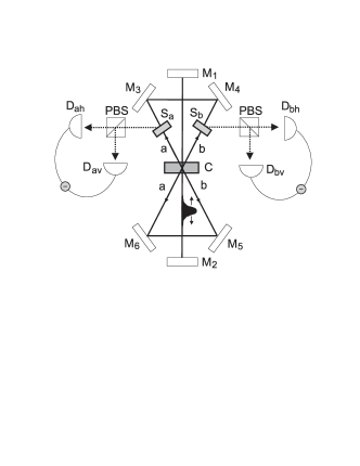
Figure 1: Proposed setup for an “entanglement laser”. An intense pump pulse propagates back and forth between the mirrors $M_{1}$ and $M_{2}$. Whenever it traverses the non-linear crystal $C$ it creates polarization entangled photon pairs into the modes $a$ and $b$, which are counter-propagating pulses inside the cavity formed by the mirrors $M_{3}$ to $M_{6}$. The cavities, which have to be interferometrically stable, are carefully adjusted such that the three pulses (pump, $a$ and $b$) always overlap in the crystal. The fact that $a$ and $b$ propagate in the same cavity automatically synchronizes the counter-propagating modes. The number of photons in $a$ and $b$ increases exponentially with the number of round-trips. They can be switched out of the cavity by electro-optic switches $S_{a}$ and $S_{b}$. The polarization of each pulse is then analyzed with the help of polarizing beam splitters (PBS) followed by photo-diodes that give a signal proportional to the number of photons. Taking the difference between the photon numbers for the two polarizations behind each PBS corresponds to a spin measurement. The axis of spin analysis is changed by appropriate wave-plates in front of the PBS.

Let us now study our system in more detail. The source of entangled light is described by a Hamiltonian kwiat

$$H=i\kappa(a^{\dagger}_{h}b^{\dagger}_{v}-a^{\dagger}_{v}b^{\dagger}_{h})+h.c.,$$ (1)

where $a$ and $b$ refer to the two conjugate directions along which the photon pairs are emitted, as shown in Fig. 1, $h$ and $v$ denote horizontal and vertical polarization, and $\kappa$ is a coupling constant whose magnitude depends on the nonlinear coefficient of the crystal and on the intensity of the pump pulse. The Hamiltonian describes two phase coherent twin beam sources, corresponding to the pairs of modes $a_{h},b_{v}$ and $a_{v},b_{h}$. In the absence of losses, it produces a state of the form

$$|\psi\rangle=e^{-i\hat{H}t}|0\rangle=\frac{1}{\cosh^{2}\tau}\sum_{n=0}^{\infty}\sqrt{n+1}\;\tanh^{n}\tau\;|\psi^{n}_{-}\rangle,$$ (2)

where $\tau=\kappa t$ is the effective interaction time and

$$|\psi^{n}_{-}\rangle=\frac{1}{\sqrt{n+1}}\frac{1}{n!}(a^{\dagger}_{h}b^{\dagger}_{v}-a^{\dagger}_{v}b^{\dagger}_{h})^{n}|0\rangle$$

$$=\frac{1}{\sqrt{n+1}}\sum_{m=0}^{n}(-1)^{m}|n\!\!-\!\!m\rangle_{a_{h}}|\,m\rangle_{a_{v}}|\,m\rangle_{b_{h}}|n\!\!-\!\!m\rangle_{b_{v}}\,.$$ (3)

All terms in the expansion in Eq. (3) have the same magnitude, such that the observed polarization (the difference in the number of horizontal and vertical photons) will fluctuate strongly. However, there is a perfect anti-correlation between the $a$ and $b$ pulses. The state $|\psi\rangle$ looks the same if the axis of polarization analysis is rotated by the same amount for the $a$ and $b$ modes. It is the polarization equivalent of a spin singlet state durkin , where the spin components correspond to the Stokes parameters of polarization,

$$J^{A}_{z} = \frac{1}{2}(a^{\dagger}_{h}a_{h}-a^{\dagger}_{v}a_{v}),\,\,\,J^{A}_{x}=\frac{1}{2}(a^{\dagger}_{+}a_{+}-a^{\dagger}_{-}a_{-})$$

$$J^{A}_{y} = \frac{1}{2}(a^{\dagger}_{l}a_{l}-a^{\dagger}_{r}a_{r}),$$ (4)

The spin components can thus be expressed as differences in photon numbers, where $a_{+,-}=\frac{1}{\sqrt{2}}(a_{h}\pm a_{v})$ correspond to linearly polarized light at $\pm 45^{\circ}$, and $a_{l,r}=\frac{1}{\sqrt{2}}(a_{h}\pm ia_{v})$ to left- and righthanded circularly polarized light. The label $A$ refers to the $a$ modes, cf. Fig. 1. Analogous relations express ${\bf J}^{B}$ in terms of the $b$ modes. The total spin satisfies $({\bf J}^{A})^{2}=(J^{A}_{x})^{2}+(J^{A}_{y})^{2}+(J^{A}_{z})^{2}=\frac{N_{A}}{2}\left(\frac{N_{A}}{2}+1\right)$. Number states of the modes $a_{h}$ and $a_{v}$ are eigenstates of $J^{A}_{z}$ and of $({\bf J}^{A})^{2}$. The state $|n-k\rangle_{a_{h}}|k\rangle_{a_{v}}$, has total spin $j=n/2$ and $J^{A}_{z}$ eigenvalue $m=(n-2k)/2$.

The states $|\psi^{n}_{-}\rangle$ of Eq. (3) are singlet states of the total angular momentum operator ${\bf J}={\bf J}^{A}+{\bf J}^{B}$ for fixed $j_{A}=j_{B}=n/2$. As a consequence, $\langle\psi|{\bf J}^{2}|\psi\rangle=0$ also for the state $|\psi\rangle$ of Eq. (2). Losses and imperfections lead to non-zero values for the total angular momentum, corresponding to non-perfect correlations between the Stokes parameters in the $a$ and $b$ pulses. Since the ideal state of Eq. (2) is highly entangled, one expects that states in its vicinity are still entangled. We now present a convenient criterion for entanglement: for separable states

$$\frac{\langle{\bf J}^{2}\rangle}{\langle N\rangle}\geq\frac{1}{2},$$ (5)

where ${\bf J}={\bf J}^{A}+{\bf J}^{B}$ and $N=N_{A}+N_{B}$. To prove this, consider $\langle{\bf J}^{2}\rangle$ for a separable state $\rho=\sum_{i}p_{i}\rho_{i}^{A}\otimes\sigma_{i}^{B}$. One has

$$\langle{\bf J}^{2}\rangle=\langle({\bf J}^{A})^{2}\rangle+\langle({\bf J}^{B})^{2}\rangle+2\langle{\bf J}^{A}\cdot{\bf J}^{B}\rangle$$

$$=\sum_{i}p_{i}\langle({\bf J}^{A})^{2}\rangle_{i}+\sum_{i}p_{i}\langle({\bf J}^{B})^{2}\rangle_{i}+2\sum_{i}p_{i}\langle{\bf J}^{A}\rangle_{i}\langle{\bf J}^{B}\rangle_{i}$$

$$\geq\sum_{i}p_{i}[\langle({\bf J}^{A})^{2}\rangle_{i}+\langle({\bf J}^{B})^{2}\rangle_{i}-2|\langle{\bf J}^{A}\rangle_{i}||\langle{\bf J}^{B}\rangle_{i}|]$$

$$\geq\sum_{i}p_{i}[\langle({\bf J}^{A})^{2}\rangle_{i}+\langle({\bf J}^{B})^{2}\rangle_{i}-2\alpha_{i}\beta_{i}],$$ (6)

where $\langle{\bf J}^{A}\rangle_{i}=\mbox{Tr}\rho_{i}^{A}{\bf J}^{A}$, $\langle{\bf J}^{B}\rangle_{i}=\mbox{Tr}\sigma_{i}^{B}{\bf J}^{B}$ etc. Furthermore $\alpha_{i}=\sqrt{\langle({\bf J}^{A})^{2}\rangle_{i}+\frac{1}{4}}-\frac{1}{2},\beta_{i}=\sqrt{\langle({\bf J}^{B})^{2}\rangle_{i}+\frac{1}{4}}-\frac{1}{2}$, and we have used the fact inequality that $|\langle{\bf J}\rangle|\leq\sqrt{\langle{\bf J}^{2}\rangle+\frac{1}{4}}-\frac{1}{2}$. The last line of Eq. (6) can be rewritten as

$$\sum_{i}p_{i}[\alpha_{i}^{2}+\alpha_{i}+\beta_{i}^{2}+\beta_{i}-2\alpha_{i}\beta_{i}]=\sum_{i}p_{i}[(\alpha_{i}-\beta_{i})^{2}$$

$$+\alpha_{i}+\beta_{i}]\geq\sum_{i}p_{i}[\alpha_{i}+\beta_{i}]\geq\frac{1}{2}(\langle N_{A}\rangle+\langle N_{B}\rangle),$$ (7)

where the last inequality follows from $\sqrt{\langle{\bf J}^{2}\rangle+\frac{1}{4}}-\frac{1}{2}\geq\frac{1}{2}\langle N\rangle$, which is a direct consequence of the relation ${\bf J}^{2}=\frac{N}{2}\left(\frac{N}{2}+1\right)$. Since $N=N_{A}+N_{B}$, this concludes the proof of our criterion. Thus every state that has $\langle{\bf J}^{2}\rangle/\langle N\rangle<\frac{1}{2}$ is entangled. This is a tight bound. There are separable states that reach $\langle{\bf J}^{2}\rangle/\langle N\rangle=\frac{1}{2}$, for example the product state $|2j\rangle_{a_{h}}|0\rangle_{a_{v}}|0\rangle_{b_{h}}|2j\rangle_{b_{v}}$, which in spin notation corresponds to $|j_{A}=j,m_{A}=j\rangle\otimes|j_{B}=j,m_{B}=-j\rangle$.

It should be emphasized that our criterion is sufficient, but not necessary. There are entangled states that are not approximate singlets. Our criterion is specifically designed for the class of states under consideration and for polarization observables. It has some similarity to the entanglement criterion for spin-squeezed states derived in Ref. sorensen . The quantities $\langle{\bf J}^{2}\rangle$ and $\langle N\rangle$ are simple to calculate, such that the effects of various imperfections can be studied with ease. We start by investigating the effect of loss.

Loss in a general mode $c$ corresponds to a transformation $c\rightarrow\sqrt{\eta}\,c+\sqrt{1-\eta}\,d$, where $d$ is an empty mode and $\eta$ is the transmission coefficient. Let us start by assuming that the modes $a_{h}$ and $a_{h}$ suffer an equal amount of loss described by $\eta_{A}$, while the $b$ modes have a transmission $\eta_{B}$. Using Eq. (4) this leads to the following transformations:

$$\langle({\bf J}^{A,B})^{2}\rangle \rightarrow \eta_{A,B}^{2}\langle({\bf J}^{A,B})^{2}\rangle+\frac{3}{4}\eta_{A,B}(1-\eta_{A,B})\langle N_{A,B}\rangle$$

$$\langle{\bf J}^{A}\cdot{\bf J}^{B}\rangle \rightarrow \eta_{A}\eta_{B}\langle{\bf J}^{A}\cdot{\bf J}^{B}\rangle.$$ (8)

The state before losses, Eq. (2), has $\langle({\bf J}^{A})^{2}\rangle=\langle({\bf J}^{B})^{2}\rangle=-\langle{\bf J}^{A}\cdot{\bf J}^{B}\rangle$, $\langle N_{A}^{2}\rangle=\langle N_{B}^{2}\rangle=\langle N_{A}N_{B}\rangle$ and $\langle N_{A}\rangle=\langle N_{B}\rangle=\langle N\rangle/2$, which leads to the following expression for the total angular momentum after losses:

$$\langle{\bf J}^{2}\rangle\rightarrow(\Delta\eta)^{2}\langle({\bf J}^{A})^{2}\rangle+\frac{3}{8}[\eta_{A}(1-\eta_{A})+\eta_{B}(1-\eta_{B})]\langle N\rangle,$$ (9)

where $\Delta\eta=\eta_{A}-\eta_{B}$. Remembering that $({\bf J}^{A})^{2}=\frac{N_{A}}{2}(\frac{N_{A}}{2}+1)$ one sees that the first term in Eq. (9), which depends on $\Delta\eta$, is of order $\langle N\rangle^{2}$, while the second term is only $O(\langle N\rangle)$. If one wants to observe entanglement for large photon numbers, it is therefore important for the losses (including detection efficiencies) in the $a$ and $b$ modes to be well balanced. More precisely, Eq. (9) together with our entanglement criterion implies the condition $\Delta\eta\lesssim\frac{2\sqrt{2}}{\sqrt{\langle N\rangle}}$. An equivalent requirement was met for $\langle N\rangle$ of order $10^{6}$ in the experiment of Ref. smithey that demonstrated the strong photon number correlations of pulsed twin beams by direct integrative detection. An analogous condition can be derived for a difference in losses between different polarization modes. If all modes suffer the same amount of loss, described by a transmission $\eta$, then only the second term in Eq. (9) remains, leading to a loss-induced correction to the ratio $\langle{\bf J}^{2}\rangle/\langle N\rangle$ of $\frac{3(1-\eta)}{4}$, taking into account that the losses also transform $\langle N\rangle$ into $\eta\langle N\rangle$. This gives a critical transmission value $\eta_{c}=1/3$, above which entanglement is provable by our criterion. The entanglement is thus surprisingly robust under balanced losses.

So far we have considered a situation where first the ideal state of Eq. (2) is created, and then it is subjected to loss. However, in the cavity setup of Fig. 1, which is required to achieve high photon numbers, photon creation (in the non-linear crystal) and loss (in the crystal and all other optical elements) happen effectively simultaneously. It is convenient to transform to a new basis of modes given by $c_{1}=\frac{1}{\sqrt{2}}(a_{h}+b_{v}),c_{2}=\frac{1}{\sqrt{2}}(a_{h}-b_{v}),c_{3}=\frac{1}{\sqrt{2}}(a_{v}+b_{h}),c_{4}=\frac{1}{\sqrt{2}}(a_{v}-b_{h})$. In this basis the Hamiltonian (1) becomes that of four independent, but phase-coherent, squeezers, $H=\frac{i\kappa}{2}\left((c_{1}^{\dagger})^{2}-(c_{2}^{\dagger})^{2}-(c_{3}^{\dagger})^{2}+(c_{4}^{\dagger})^{2}+h.c.\right)$. Introducing the quadrature operators $x_{i}=\frac{1}{\sqrt{2}}(c_{i}+c_{i}^{\dagger}),p_{i}=-\frac{i}{\sqrt{2}}(c_{i}-c_{i}^{\dagger})$ gives

$$H=\frac{\kappa}{2}\left(x_{1}p_{1}-x_{2}p_{2}-x_{3}p_{3}+x_{4}p_{4}\right)+h.c.$$ (10)

Writing down the Heisenberg equations for this Hamiltonian, $\dot{x}_{1}=i[H,x_{1}]$ etc., one sees that $\langle p_{1}^{2}\rangle,\langle x_{2}^{2}\rangle,\langle x_{3}^{2}\rangle$ and $\langle p_{4}^{2}\rangle$ become squeezed exponentially, while the fluctuations in the conjugate quadratures, $\langle x_{1}^{2}\rangle,\langle p_{2}^{2}\rangle,\langle p_{3}^{2}\rangle,\langle x_{4}^{2}\rangle$ grow correspondingly. In the presence of losses, the Heisenberg equations have to be replaced by Langevin equations of the form

$$\dot{x}_{1}=\kappa(t)x_{1}-\lambda x_{1}+f_{x1}(t)$$

$$\dot{p}_{1}=-\kappa(t)p_{1}-\lambda p_{1}+f_{p1}(t),$$ (11)

and corresponding equations for the other modes. Here the time dependence of $\kappa(t)=\kappa_{0}e^{-\Lambda t}$ takes into account the loss of the pump beam while $\lambda$ is the loss rate of the down-converted light; $f_{x1}(t)$ and $f_{p1}(t)$ are the quantum noise operators associated with the losses scully , satisfying $\langle f_{x1}(t)f_{x1}(t^{\prime})\rangle=\langle f_{p1}(t)f_{p1}(t^{\prime})\rangle=-i\langle f_{x1}(t)f_{p1}(t^{\prime})\rangle=\lambda\delta(t-t^{\prime})$. Here we have assumed that the loss rate $\lambda$ is the same for all four down-conversion modes $a_{h},a_{v},b_{h},b_{v}$. We will discuss the case of unbalanced loss rates below.

Eqs. (11) can be integrated explicitly, leading to

$$x_{1}(t)=e^{\int_{0}^{t}k(t^{\prime})dt^{\prime}}x_{1}(0)+\int_{0}^{t}dt^{\prime}e^{\int_{t^{\prime}}^{t}k(t^{\prime\prime})dt^{\prime\prime}}f_{x_{1}}(t^{\prime}),$$ (12)

where $k(t)=\kappa(t)-\lambda$ and $\int\limits_{t^{\prime}}^{t}\kappa(t^{\prime\prime})dt^{\prime\prime}=\frac{\kappa_{0}}{\Lambda}(e^{-\Lambda t^{\prime}}-e^{-\Lambda t})$. There is a corresponding expression for $p_{1}(t)$ where the sign of $\kappa(t)$ is flipped.

To understand what these results imply for the polarization entanglement, one can express the angular momentum in terms of the quadratures $x_{i},p_{i}$. One finds

$$J_{z}=\frac{1}{2}(x_{1}x_{2}+p_{1}p_{2}-x_{3}x_{4}-p_{3}p_{4})$$

$$J_{x}=\frac{1}{2}(x_{1}x_{3}+p_{1}p_{3}+x_{2}x_{4}+p_{2}p_{4})$$

$$J_{y}=\frac{1}{2}(-x_{1}p_{4}+x_{4}p_{1}-x_{2}p_{3}+x_{3}p_{2}).$$ (13)

Introducing the generic notation $p$ for the quadratures that are squeezed (which are $p_{1},x_{2},x_{3},p_{4}$) and $x$ for those whose fluctuations grow exponentially (which are $x_{1},p_{2},p_{3},x_{4}$), one sees that all terms in Eq. (13) have the generic form $x\cdot p$, and one finds $\langle{\bf J}^{2}\rangle=3(\langle x^{2}\rangle\langle p^{2}\rangle-\frac{1}{4})$. The total photon number $N=\frac{1}{2}\sum_{i}(x_{i}^{2}+p_{i}^{2}-1)$, leading to

$$\frac{\langle{\bf J}^{2}\rangle}{\langle N\rangle}=\frac{3}{2}\cdot\frac{\langle x^{2}\rangle\langle p^{2}\rangle-\frac{1}{4}}{\langle x^{2}\rangle+\langle p^{2}\rangle-1}.$$ (14)

Fig. 2 shows the expected time development of the mean photon number $\langle N\rangle$ and the ratio $\langle{\bf J}^{2}\rangle/\langle N\rangle$ as determined from Eqs. (14) and (12) for realistic parameter values. The experimentally achievable value for $\kappa$ can be estimated by extrapolating existing experimental results lamas to higher pump laser intensities. A value of $\tau=\kappa t=1$ for a single pass through a 2mm BBO crystal is realistic with weakly focussed pump pulses of a few $\mu$J, which is still below the optical damage threshold. The cavity design of Fig. 1 including switching elements will have loss rates on the percent level. Fig. 2 shows that very high photon numbers can be achieved with just a few round-trips. If balanced losses are the only imperfection, then the entanglement is very strong even for large photon numbers, as long as the “laser” is far above threshold, i.e. as long as the rate of creation of entangled photon pairs is much larger than the loss rate ($\kappa/\lambda\gg 1$). Note that we are interested in the onset regime, far from saturation (depletion of the pump).

The photon number $\langle N\rangle$ is limited by the requirement of observing entanglement in the presence of other imperfections. In particular, Fig. 2 shows the effect of a difference in the loss rates between the $a$ and $b$ modes. Suppose that the modes $a_{h}$ and $a_{v}$ have one loss rate $\lambda_{A}$, while $b_{h}$ and $b_{v}$ have a different one $\lambda_{B}$. Then the quadratures $x_{i},p_{i}$ no longer diagonalize the system. For example, $x_{1}$ and $x_{2}$ satisfy the coupled equations

$$\dot{x}_{1}=\kappa(t)x_{1}-\bar{\lambda}x_{1}-\frac{\Delta\lambda}{2}x_{2}+f_{x_{1}}(t)$$

$$\dot{x}_{2}=-\kappa(t)x_{2}-\bar{\lambda}x_{2}-\frac{\Delta\lambda}{2}x_{1}+f_{x_{2}}(t),$$ (15)

where $\bar{\lambda}=\frac{1}{2}(\lambda_{A}+\lambda_{B}),\Delta\lambda=\lambda_{A}-\lambda_{B}$ and $f_{x_{1},x_{2}}$ are the appropriate noise operators. There are analogous coupled equations for the pairs $p_{1}$ and $p_{2}$, $x_{3}$ and $x_{4}$, and $p_{3}$ and $p_{4}$. These equations are diagonal for a new basis of modes $\xi_{i},\pi_{i}$ that is related to the $x_{i},p_{i}$ by a small rotation, which for $\Delta\lambda\ll\kappa$ takes the simple form: $x_{1}=\xi_{1}+(\Delta\lambda/4\kappa)\xi_{2},x_{2}=-(\Delta\lambda/4\kappa)\xi_{1}+\xi_{2},x_{3}=\xi_{3}-(\Delta\lambda/4\kappa)\xi_{4},x_{4}=(\Delta\lambda/4\kappa)\xi_{3}+\xi_{4}$, and identical equations for the $p_{i}$ in terms of the $\pi_{i}$. In analogy to the case of balanced losses, the quadratures $\xi_{1},\pi_{2},\pi_{3}$ and $\xi_{4}$ grow exponentially, while the quadratures $\pi_{1},\xi_{2},\xi_{3}$ and $\pi_{4}$ become squeezed. Substituting the above expressions for the $x_{i},p_{i}$ into Eq. (13) one finds that, due to the small rotation between the old and new diagonal modes, the $J_{i}$ contain terms that are quadratic in the new large quadratures $(\xi_{1},\pi_{2},\pi_{3},\xi_{4})$. This leads to an $O(\langle N\rangle^{2})$ contribution to ${\bf J}^{2}$. The dominating correction to the ratio $\langle{\bf J}^{2}\rangle/\langle N\rangle$ is $\frac{(\Delta\lambda)^{2}}{32\kappa^{2}}\langle N\rangle$, leading to the condition $\frac{\Delta\lambda}{\kappa}\lesssim\frac{4}{\sqrt{\langle N\rangle}}$ for observing entanglement. In the regime far above threshold, where $\lambda\ll\kappa$, this is fairly easy to satisfy even for very large photon numbers.

The effects of other imperfections can be studied in similar ways. The most important one is a phase mismatch between the two twin beams, i.e. a Hamiltonian $H=i\kappa(a^{\dagger}_{h}b^{\dagger}_{v}-e^{i\phi}a^{\dagger}_{v}b^{\dagger}_{h})+h.c.$ instead of Eq. (1). This can be brought to the ideal form by a transformation $a^{\dagger}_{v}\rightarrow e^{-i\phi/2}a^{\dagger}_{v}$, $b^{\dagger}_{h}\rightarrow e^{-i\phi/2}b^{\dagger}_{h}$, which is equivalent to $c_{3}\rightarrow e^{i\phi/2}c_{3}$, $c_{4}\rightarrow e^{i\phi/2}c_{4}$. This corresponds to a rotation of the quadratures $x_{3}\rightarrow\cos\frac{\phi}{2}x_{3}-\sin\frac{\phi}{2}p_{3}$, $p_{3}\rightarrow\sin\frac{\phi}{2}x_{3}+\cos\frac{\phi}{2}p_{3}$, and analogously for $x_{4},p_{4}$. Similarly to the case of unbalanced losses, this gives a correction to the ratio $\langle{\bf J}^{2}\rangle/\langle N\rangle$ whose dominant term is $\frac{1}{16}\phi^{2}\langle N\rangle$, leading to a condition $\phi\lesssim\frac{4}{\sqrt{3}\langle N\rangle}$ for observing entanglement. This means that strong entanglement of a million photons can be observed if $\phi$ is of order $\pi/1000$. This level of precision of optical phases is challenging, but conceivable. Strong entanglement for smaller, but still considerable, photon numbers is correspondingly easier to achieve.

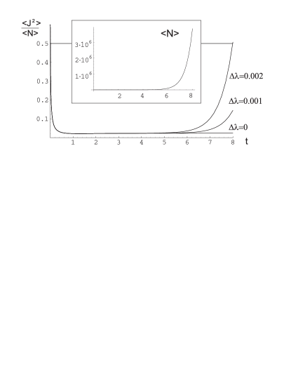
Figure 2: Time development of the ratio $\langle{\bf J}^{2}\rangle/\langle N\rangle$ and of the mean photon number $\langle N\rangle$. The units are chosen such that $t=1$ corresponds to a single pass through the crystal. The initial photon creation rate $\kappa_{0}=1$, the mean downconverted photon loss rate $\bar{\lambda}=0.03$ and the pump loss rate $\Lambda=0.01$. After 8 passes $\langle N\rangle$ reaches the range of millions. The ratio $\langle{\bf J}^{2}\rangle/\langle N\rangle$ is shown for three different values of the loss rate imbalance $\Delta\lambda$, namely 0, 0.001 and 0.002.

An amplitude mismatch in the Hamiltonian, $H=i\kappa(a^{\dagger}_{h}b^{\dagger}_{v}-fa^{\dagger}_{v}b^{\dagger}_{h})+h.c.$ with $f$ real, leads to a different degree of squeezing for the modes $c_{1},c_{2}$ compared to the modes $c_{3},c_{4}$, but not to a rotation of the quadrature amplitudes, such that the effect on $\langle{\bf J}^{2}\rangle/\langle N\rangle$ does not grow with $\langle N\rangle$.

Another relevant imperfection is a birefringence-related mode mismatch, corresponding to a Hamiltonian $H=i\kappa(a^{\dagger}_{h}\tilde{b}^{\dagger}_{v}-\tilde{a}^{\dagger}_{v}b^{\dagger}_{h})+h.c.$, where the spatio-temporal modes $\tilde{a}$ and $\tilde{b}$ of the vertical light differ slightly from the modes $a$ and $b$ of the horizontal light. In analogy to the case of losses, one can show that a mode mismatch that affects the $a$ and $b$ modes in a symmetric way leads to a correction to $\langle{\bf J}^{2}\rangle/\langle N\rangle$ that does not grow with $\langle N\rangle$, which implies that the birefringence-related walk-off, while important, does not have to be reduced by orders of magnitude with respect to experiments on the few-photon level. As before, an asymmetry leads to an $O(\langle N\rangle)$ effect. Note that the other major errors that we have discussed, including the phase mismatch, are also related to symmetry breaking between the $a$ and $b$ modes. In general, geometric symmetry between the $a$ and $b$ modes should be implementable to very high accuracy for the setup of Fig. 1.

In conclusion, the goal of producing strongly entangled singlet-like states of very large photon numbers seems realistic with our proposed system. Besides extending the domain where quantum phenomena have been observed, such states would also have interesting applications, for example in quantum cryptography durkin . We would like to thank W. Irvine, A. Lamas-Linares and F. Sciarrino for useful comments. C.S. is supported by a Marie Curie fellowship of the European Union (HPMF-CT-2001-01205).

References

• (1) L.-A. Wu, H.J. Kimble, J.L. Hall, and H. Wu, Phys. Rev. Lett. 57, 2520 (1986); H.J. Kimble and D.F. Walls (Eds.), Squeezed States of the Electromagnetic Field, special issue of J. Opt. Soc. Am. B 4, 1453 (1987); R. Loudon and P.L. Knight (Eds.), Squeezed Light, special issue of J. Mod. Opt. 34, 709 (1987).
• (2) A. Heidmann et al., Phys. Rev. Lett. 59, 2555 (1987); C. Fabre and E. Giacobino (Eds.), Quantum Noise Reduction in Optical Systems/Experiments, special issue of Appl. Phys. B 55, 189 (1992).
• (3) D.T. Smithey, M. Beck, M. Belsley, and M.G. Raymer, Phys. Rev. Lett. 69, 2650 (1992).
• (4) W.P. Bowen, N. Treps, R. Schnabel, and P.K. Lam, Phys. Rev. Lett. 89, 253601 (2002); see also N. Korolkova, G. Leuchs, R. Loudon, T.C. Ralph, and Ch. Silberhorn, Phys. Rev. A 65, 052306 (2002).
• (5) A. Lamas-Linares, J.C. Howell, and D. Bouwmeester, Nature (London) 412, 887 (2001).
• (6) P.G. Kwiat, K. Mattle, H. Weinfurter, A. Zeilinger, A.V. Sergienko, and Y. Shih, Phys. Rev. Lett. 75, 4337 (1995).
• (7) G.A. Durkin, C. Simon, and D. Bouwmeester, Phys. Rev. Lett. 88, 187902 (2001).
• (8) The inequality $|\langle{\bf J}\rangle|\leq\sqrt{\langle{\bf J}^{2}\rangle+\frac{1}{4}}-\frac{1}{2}$ can be rewritten more intuitively as $\langle{\bf J}^{2}\rangle\geq|\langle{\bf J}\rangle|^{2}+|\langle{\bf J}\rangle|$. One can always rotate the axes of the coordinate system such that only $\langle J_{z}\rangle$ is different from zero. The claim is obviously true for a pure state of fixed total spin $j$. A pure state that is a superposition of components with different $j$ values is effectively a mixed state, because off-diagonal terms between different $j$ do not contribute to $\langle{\bf J}\rangle$ and $\langle{\bf J}^{2}\rangle$. For mixed states $\rho=\sum p_{i}\rho_{i}$ we have $\sum p_{i}\langle{\bf J}^{2}\rangle_{i}\geq\sum p_{i}[m_{i}^{2}+m_{i}]$, where we have introduced the notation $m_{i}=|\langle{\bf J}\rangle_{i}|$. Noting that $|\langle{\bf J}\rangle_{\rho}|=|\sum p_{i}\langle{\bf J}\rangle_{i}|\leq\sum p_{i}m_{i}$ and that $\sum p_{i}m_{i}^{2}\geq(\sum p_{i}m_{i})^{2}$ one obtains the desired inequality.
• (9) A. SΓΈrensen, L.-M. Duan, J.I. Cirac, and P. Zoller, Nature 409, 63 (2001).
• (10) See e.g. M.O. Scully and M.S. Zubairy, Quantum Optics (Cambridge University Press, Cambridge, 1997).